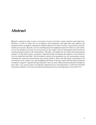
This document describes the development of a magnetic component design environment. It includes the development of an automated core loss measurement system to characterize magnetic materials, a database to store measurement data, and a design software tool. The core loss measurement system allows for easy and automated measurement of core loss over a range of frequencies and flux densities. Measured data is stored in a database, which can be accessed by the design software to enable accurate prediction of core losses during the design process. Validation measurements on inductors showed errors between predicted and measured losses and temperatures were less than 10%, demonstrating the effectiveness of the design environment for improving magnetic component design.


![Chapter 2
Magnetic Materials Overview and
Comparison
The history of magnetism begins in the 6th century B.C. when the Greek philosopher Thales discovered
magnetic properties of a mineral called magnetite. He noticed that his walking stick that had a metal ending
was attracted by a rock made of magnetite. However, the first scientific study on magnetism was published
in 1600 by William Gilbert, where the physical background of magnetic forces was explained. Later, the
science of electromagnetism was shaped by scientists like Faraday, Maxwell, Oersted and Hertz.
Parallel to the developments in the magnetic theory, considerable attention was focused on understanding
different magnetic materials and producing materials with desirable characteristics. Since the performance
of magnetic components used in power electronics and in other fields of electrical engineering greatly de-
pends on material characteristics, there is always a need to produce materials with better characteristics.
However, there is no perfect magnetic material that would meet all the designers requirements. Therefore
designing magnetic components is always a tradeoff between cost, size and performance indexes. Because
of this, knowing the characteristics of different magnetic materials and their advantages and disadvantages
is essential for the process of designing magnetic components.
This chapter gives a systematic overview of the magnetic materials used in modern day power elec-
tronics. It lists advantages and disadvantages of different material groups. This gives the basis for their
comparison, which is a first step in magnetic component design. Moreover, manufacturing processes for
each of the groups are described. This is important for better understanding all the differences and similari-
ties between different material groups.
2.1 Classification of Magnetic Materials
According to their magnetic properties, all materials can be classified in three groups [1], [3]:
• Diamagnetic materials
• Paramagnetic materials
3](https://image.slidesharecdn.com/b2c598c0-acc4-4f16-a555-962d4c8820c3-160325211659/85/Final_report-17-320.jpg)
![CHAPTER 2. MAGNETIC MATERIALS OVERVIEW AND COMPARISON
Diamagnetic Paramagnetic Ferromagnetic
Superconductor Cesium Cobalt
Graphite Aluminum Iron
Copper Lithium Nickel
Lead Magnesium
Silver Sodium
Water
Table 2.1: Some typical representatives of diamagnetic, paramagnetic and ferromagnetic materials.
• Ferromagnetic materials
Diamagnetic materials (Diamagnets) are materials that have magnetic permeability less than µ0 (relative
permeability is less than 1). These materials cause the lines of magnetic flux to curve away from the ma-
terial and hence it appears as they create a magnetic field opposed to an external magnetic field. Such a
behavior is common to most of materials present in nature (and often these materials are referred to as non-
magnetic). However, the effect of repulsion when exposed to external magnetic field is so weak that it is
usually not noticed at all. The only exceptions are superconductors which completely exclude the lines of
magnetic flux and can be regarded as perfect diamagnets.
Paramagnetic materials (Paramagnets) have relative permeability slightly higher than one. These ma-
terials are slightly magnetized in the presence of external magnetic field. However, in the absence of the
external magnetic field these materials retain no magnetization.
Ferromagnetic materials (Ferromagnets) have relative permeability much greater than one (typically
from 10 to 100000) [1]. These materials get magnetized in the presence of an external magnetic field and
unlike paramagnets do not immediately get demagnetized when the external field is removed. Ferromag-
netic materials are the only ones that can be used to produce considerable magnetic forces. These forces can
be noticed and felt and they are the ones that are generally associated with the phenomenon of magnetism
encountered in everyday life. These materials are relevant for the design of magnetic components for power
electronics. Some typical diamagnetic, paramagnetic and ferromagnetic materials found in nature are listed
in Table 2.1.
Ferromagnetic materials can be further divided into two groups depending on their coercive force (Hc)
[1],[3]. These two groups are:
• Hard magnetic materials
• Soft magnetic materials
According to [1], hard magnetic materials are those that have Hc > 10000 A/m. These materials are often
called permanent magnets. Usually they also have very high value for remanent induction Br. Therefore,
these materials are very hard to demagnetize (hence the name permanent magnets). Typical applications of
such materials are for electrical motors and generators, sensing devices and mechanical holding.
Soft magnetic materials typically have Hc < 1000 A/m. Therefore, they are characterized by much
narrower BH loops compared to hard magnetic materials. Moreover, it is much easier to change magnetic
alignment in the structure of these materials. They are widely used in modern electrical engineering and
4](https://image.slidesharecdn.com/b2c598c0-acc4-4f16-a555-962d4c8820c3-160325211659/85/Final_report-18-320.jpg)
![CHAPTER 2. MAGNETIC MATERIALS OVERVIEW AND COMPARISON
electronic applications. In fact, most of magnetic components in power electronics use cores made of these
materials.
Materials that have Hc in the range of 1000 – 10000 A/m are considered to be somewhat between soft
and hard, however there is no general term that would describe such materials [3]. These materials are
mainly used as recording media.
Since soft magnetic materials are the most relevant for power electronics, we will mainly focus on them.
They can be further divided into two groups based on their chemical composition:
• Ferrites (ferrimagnetic materials)
• Iron (Fe) based soft magnetic materials (ferromagnetic materials in narrow sense)
Here it is important to stress the difference between the terms, since often in literature soft magnetic ma-
terials based on iron are referred to as ferromagnetic although they, together with ferrimagnetic materials,
belong to the larger group of ferromagnetic materials. However it is often said that soft magnetic materials
based on iron are ferromagnetic materials in narrow sense [1].
Ferrimagnetic materials (ferrites) are ceramic materials made from oxides of iron and metals like man-
ganese (Mn), zinc (Zn) and nickel (Ni). Their main advantage is high electrical resistivity and relatively low
losses at high frequencies. However, these materials have quite low saturation flux density.
Ferromagnetic materials are made of metal alloys of iron and metals like silicon (Si), nickel, chrome
(Cr) and cobalt (Co). They have higher saturation flux density than ferrites, but also much higher electrical
conductivity (therefore higher losses due to eddy currents). This group of materials can be further divided
into several subgroups based on the manufacturing technology and material properties:
• Iron based alloys
• Powder iron
• Amorphous alloys
• Nanocrystalline alloys
The order in which these different material groups are listed corresponds to chronological order in which
they appeared and in which they have been manufactured and used in power electronics. Iron based alloys
are metal alloys of iron and silicon, nickel or cobalt. Powder iron cores are made from small iron (or other
material containing iron) particles which are mutually electrically isolated. Amorphous alloys are iron or
cobalt based alloys with special crystalline structure. They do not have crystal structure characteristic for
metals, but amorphous structure typical for glass or liquids. Nanocrystalline alloys are two phase materials
which have an amorphous alloy as a minority phase and FeSi crystals embedded into this amorphous phase.
Manufacturing processes as well as characteristics of these materials are given in the following sections.
Figure 2.1 illustrates described classification of magnetic materials
5](https://image.slidesharecdn.com/b2c598c0-acc4-4f16-a555-962d4c8820c3-160325211659/85/Final_report-19-320.jpg)

![CHAPTER 2. MAGNETIC MATERIALS OVERVIEW AND COMPARISON
Material Chemical comp. Curie temp. [◦C] Initial perm. Saturation flux density [T]
Magnesil 3%Si 97%Fe 750 1.5 K 1.5 – 1.8
Supremalloy 79%Ni 17%Fe 4%Mo 460 10 –50 K 0.66 – 0.82
Permalloy 80 78%Ni 17%Fe 5%Mo 460 12 – 100 K 0.65 – 0.82
Orthanol 50%Ni 50%Fe 500 2 K 1.42 – 1.58
Supermdur 49%Co 49%Fe 2%V 940 0.8 K 1.9 – 2.2
Table 2.2: Iron based alloys produced by Magnetics (data taken from [2] and [10]).
kilograms) the most used magnetic materials [2].
The main reason why silicon is added to iron is to reduce the conductivity and therefore reduce eddy
current loses. In addition, adding silicon reduces magnetostriction, and hence reduces the acoustic noise
caused by mechanical stress in material as a result of changing magnetic field. However, adding silicon also
has some negative effects. It reduces the saturation flux density, and can make the material lifetime shorter.
Also, adding more silicon results in a material that is very brittle. According to [1] the maximal percentage
of silicon that can be added to steel and that the material still keeps useful properties is 6.5 %. However,
iron-silicon alloy mostly used today is the one with 3 % silicon content.
Special kind of iron-silicon alloy is grain oriented silicon steel. This material has much higher perme-
ability and much lower loses in one direction than in the other. This is used when forming cores out of
this material. Namely it is always good to have lower loss and higher permeability in the direction along
the laminations, where the magnetic flux passes, than in the orthogonal direction. This property is called
anisotropy. When a magnetic material has the same magnetic properties in all directions it is called isotropic
and when this is not the case it is called anisotropic. In the last years there have been a lot of improvements
in grain oriented silicon steel manufacturing. As a result there are grain oriented silicon steel materials that
can have quite low loses in the lamination direction compared to other materials in the iron based alloys
group. Silicon steel material that is isotropic is called Non-oriented silicon steel.
Iron-nickel alloys can be made of different proportions of nickel. Today there are three different types
of iron-nickel alloys that are produced. The alloy with 80 % Ni content has very high initial permeability
(typically up to 100 K). Alloy with 50 % Ni has the highest saturation flux density in the group of iron-nickel
alloys (close to 1.6 T). And the alloy with 36 % Ni has the highest electrical resistivity in this group, also
this material has one of the smallest thermal expansion coefficient of all the magnetic materials used today.
Iron-cobalt alloys are usually made of 50 % Co. These materials have extremely high saturation flux
density (up to 2.2 T). They are used for electromagnet pole tips.
Today the greatest manufacturers of iron based alloys are Magnetics [10], Vacuumschmelze [11] and
TDK [12]. Table 2.2 gives some of the iron based alloys produced by Magnetics and lists some of their
magnetic properties. As the table shows, iron based alloys have quite high saturation flux density and offer
quite a wide range of different initial permeability values. Saturation flux density of 50 % cobalt alloy has
in fact the highest saturation flux density value among all commercially available soft magnetic materials.
In addition, these materials typically have Curie temperature greater than 450◦C and can therefore be used
at high temperatures (typically up to 150◦C in order to have a high margin to Curie temperature). Due to the
fact that these materials have been manufactured and used for many years now, their manufacturing process
has developed so that they are relatively inexpensive compared to other magnetic materials. In addition
cores of various sizes and shapes are readily available. Cores made of iron based alloy laminations are not
brittle. They are quite strong and not sensitive to mechanical wear.
7](https://image.slidesharecdn.com/b2c598c0-acc4-4f16-a555-962d4c8820c3-160325211659/85/Final_report-21-320.jpg)

![CHAPTER 2. MAGNETIC MATERIALS OVERVIEW AND COMPARISON
Cores are formed from metal ribbons, where laminations are electrically insulated. This is achieved by
coating the metal ribbon with a thin layer of electrically insulating material. Materials that also have bind-
ing properties (behave like glue) are used so that the laminations would stick together after core formation.
Toroids are then simply formed by winding the coated ribbon tape. For other core shapes (such as E shapes
for example), the core formation process is a bit more complex. For these cores building parts are formed
(parts of the shape that can be easily made by stacking laminations – like I shape for example) and then
these building parts are glued together. The laminations from which the cores are formed have defined eddy
current loses, Curie temperature, saturation flux density, mechanical and thermal properties. However, for
most of the materials the BH curve can be modified and therefore, initial permeability and core loses can be
controlled before the cores are formed.
The process in which the final BH curve of the material is formed is called annealing. In this process the
cores are heated up to high temperature, while at the same time they are exposed to external magnetic field.
During this process, final steps of crystallization in the laminations take place and depending on how long
this process lasts and what was the direction of the external magnetic field, the final BH loop is shaped. If the
lines of the external magnetic field are orthogonal to the core laminations (transversal field annealing), the
final BH curve has more round or elongated shape and when the external magnetic field is parallel to core
laminations (longitudinal field annealing), final BH curve has square shape. Figure 2.2 shows three typical
BH loop shapes that can be obtained. Nickel and cobalt alloys always need to be annealed. The same goes
square round elongated
Figure 2.2: Different BH curve shapes obtained by annealing [9].
for grained oriented silicon steel. However, there are some types of iron–silicon alloys (non-oriented silicon
steel) whose BH curve can not be altered by annealing.
After annealing the laminations and stacking them to form the cores, the cores can be considered fin-
ished. They have all the magnetic, mechanical and thermal properties well defined. However, often these
cores are further processed in order to make their use easier. This is done by further coating the cores (al-
though for iron based alloys cores often come without any coating). The most usual coating material is
nylon or plastic. Often the cores are stored in aluminum case which can be coated or not. All this is done
to give further mechanical support for the laminated core and to better facilitate automated core winding.
Figure 2.3 illustrates manufacturing process for cores made of iron based alloys.
9](https://image.slidesharecdn.com/b2c598c0-acc4-4f16-a555-962d4c8820c3-160325211659/85/Final_report-23-320.jpg)
![CHAPTER 2. MAGNETIC MATERIALS OVERVIEW AND COMPARISON
Alloy material
mixing and melting
Raw materials:
Fe, Si, Ni, Co
Hot & cold
metal rolling
Liquid
metal
0.02 – 6.4 mm
tick metal
ribbon
Core winding and
insulating
laminations
Finished coresAnnealing process
Cores consisting of many
Thin, electrically isolated
laminations
Fe-Ni and
Fe-Co alloys,
Grain oriented
silicon steal
Non-oriented silicon steal
Figure 2.3: Iron based alloy cores – manufacturing process.
2.3 Powder Iron
Classification and properties
Powder iron cores are made from very small particles of iron (or other materials containing iron) that are
bound together and electrically isolated. This significantly reduces electrical conductivity of the material (10
to 100 times compared to iron based alloys) and hence eddy current losses are reduced. The fact that cores
are made of small isolated particles means that these cores have an air gap that is distributed throughout
the core. The distance between the particles (or the thickness of isolation between them) determines the
size of the distributed air gap and also the permeability of the material. A with a wide range of different
permeability are offered.
According to [2], iron powder cores were patented and their production began at the beginning of the
20th century. Since that time, manufacturing process of iron powder cores has not changed much, but the
materials used have been thoroughly researched and improved. Today iron powder cores are extensively
used in many fields of power electronics and electrical engineering.
According to their chemical composition all powder iron materials can be divided into 4 groups:
• Molypermalloy (MPP)
• High flux (HF)
• Sendust
• Pure iron powder
Here one clarification is in order. We refer to the whole group as powder iron in this thesis because of
historical and consistency reasons. However, as can be seen pure iron powder is only one subgroup, while
also other materials are classified as powder iron. Due to the fact that the pure iron powder appeared first
and as the manufacturing process is very similar for all the subgroups, in literature all these materials are
10](https://image.slidesharecdn.com/b2c598c0-acc4-4f16-a555-962d4c8820c3-160325211659/85/Final_report-24-320.jpg)
![CHAPTER 2. MAGNETIC MATERIALS OVERVIEW AND COMPARISON
Material Chemical comp. Curie temp. [◦C] Initial perm. Saturation flux density [T]
MPP 80%Ni 20%Fe 450 14 – 550 K 0.7
High Flux 50%Ni 50%Fe 360 14 – 160 K 1.5
Sendust 85%Fe 9%Si 6%Al 740 26 – 125 K 1
Pure Iron Powder 100%Fe 770 4 – 100 K 0.5 – 1.4
Table 2.4: Iron powder materials (data taken from [2] and [4]).
MPP High flux Sendust Iron Powder
Core loss Lowest Moderate Low High
Perm. vs. DC bias Better Best Good Good
Temperature stability Best Very Good Very Good Fair
Relative cost High Medium Low Lowest
Table 2.5: Comparison of different iron powder materials (adapted from [4]).
referred as powder iron [1], [2]. So the same group name is kept in this thesis.
Molypermalloy (MPP) powder cores are made of 80 % nickel and 20 % iron. These cores can have
extremely high initial permeability (up to 550 K). In addition this material has the smallest loses compared
to other iron powder materials. However, the saturation flux density is smaller than for other materials.
Also, its relative cost is the highest in this group. These cores are mainly used for in-line noise filters, high
Q filters and resonant circuits [4].
High flux (HF) powder cores are made of 50 % nickel and 50 % iron. They have the highest saturation
flux density in the group (twice higher than MPP). However, they have higher core loses when compared to
MPP. Main applications of this material are for switching regulator inductors, in-line noise filters, fly back
transformers, power factor correction (PFC), and pulse transformers [4].
Sendust powder cores are made of 85 % iron, 9 % silicon and 6 % aluminum. This material has high
saturation flux density (1 T). It has losses lower than HF and a price that is lower both than prices for MPP
and HF. One of the advantages of this material is that it has almost no magnetostriction which makes it
useful in applications operating at audible frequencies [4].
Pure iron powder cores are made from 100 % iron particles. This was the first, material to be produced
and used in this group. This material has high saturation flux density and is cheaper compared to all three
materials mentioned before. However, it also has much higher losses. This material is mostly used for
electromagnetic interference filters and low-frequency chokes in switched-mode power supplies [5]. Table
2.4 lists some of the magnetic properties of these materials.
Table 2.5 summarizes advantages and disadvantages of different iron powder materials.
Biggest manufacturers of powder iron cores are Magnetics and Micrometals [13]. Furthermore, there
is a great number of smaller companies producing powder iron cores with almost the same specifications
as for the cores from these two manufacturers. The main advantage of these materials is that they have a
high saturation flux density, offer a great variety of initial permeability values (even up to 550 K), and have
lower losses compared to iron based alloys (although pure iron powder has loses that are comparable to loses
of iron based alloys). In addition, all the materials apart from pure iron powder have more than 10 times
lower electric conductivity and therefore much lower eddy current loses. Because of all this, these materials
are well suited for high frequency applications. They are relatively inexpensive and cores are available in
11](https://image.slidesharecdn.com/b2c598c0-acc4-4f16-a555-962d4c8820c3-160325211659/85/Final_report-25-320.jpg)
![CHAPTER 2. MAGNETIC MATERIALS OVERVIEW AND COMPARISON
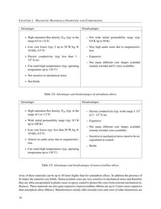
Advantages Disadvantages
+ High saturation flux density Bsat (typ. in the
range 0.8 to 1.5 T)
+ Wide initial permeability range (typ. 300 up
to 550 K)
+ Low core losses (only for certain materials)
(typ. 0.02 up to 250 W/kg @ 10 kHz, 0.5 T)
+ Low audio noise due to magnetostriction
+ Inexpensive
+ Cores produced in many different shapes
– High electric conductivity (typ. 2·104 to 1.5·
106 S/m)
– Can not stand high temperatures (typ. oper-
ating temperature < 110◦C)
– Fragile and sensitive to mechanical stress
– Brittle
– No large cores available
Table 2.6: Advantages and disadvantages of iron powder cores.
many shapes. However, big cores are not available. In addition, magnetostriction is quite low (and for
some material types almost not existing), so there is no audio noise problem. One of the advantages often
mentioned by manufacturers is that these materials exhibit soft saturation (no abrupt change in the slop of
the BH curve when saturating), which can be a great advantage in certain applications [4], [5].
Although these materials have lower electric conductivity than iron based alloys, it is still quite high
compared to ferrites and amorphous based alloys. In addition, due to the way the cores are manufactured
they can not stand very high temperatures. The main reason for this is that binding materials used to form the
cores are very sensitive to high temperatures. Therefore, exposing cores to high temperatures for long time
significantly reduces material lifetime. Manufacturers usually give a maximal temperature value that does
not affect the lifetime of the material (typically in the range of 90 to 110◦C [4],[5]). Furthermore, the cores
are quite sensitive to mechanical stress and can easily break. Table 2.6 lists advantages and disadvantages
of powder iron materials.
Manufacturing process
Manufacturing process for iron powder cores is not complex, and has not changed too much since the time
these materials were produced for the first time. This contributes to their relatively low price. Manufacturing
process starts with raw material preparation. For pure iron powder, iron with low carbon content is used.
For other materials, metals consisting of appropriate proportion of nickel and iron or silicon and iron are
used. These raw materials are then milled to obtain the powder with uniform particle size. Typical size of
powder particles after milling is in the range of 0.5 – 15 µm.
The next step in manufacturing process is the creation of the isolation layer around each of the particles.
This is achieved by treating the powder with acids, which creates a layer of oxide around each particle.
The amount of acid used determines the thickness of electrically isolating oxide layer around particles. On
the other hand this thickness determines the size of the distributed air gap (and therefore material initial
12](https://image.slidesharecdn.com/b2c598c0-acc4-4f16-a555-962d4c8820c3-160325211659/85/Final_report-26-320.jpg)
![CHAPTER 2. MAGNETIC MATERIALS OVERVIEW AND COMPARISON
permeability) as well as the electrical conductivity of the material. Therefore, by controlling the amount of
acids added, it is possible to control the size of the air gap and electric conductivity. In this process various
acids are used. The acid to be used to get the best performance is still a topic of extensive research.
After the powder has been treated with appropriate amount of acids, cores are formed from the powder.
This is done by adding binding materials and by pressing. Mostly used binding material is resin binder,
which can not stand high temperature. This is the main reason for lower maximal operating temperature
that these materials have compared to other magnetic materials. However, ways on how to improve binding
material properties are constantly researched and it is reasonable to expect improvements in this aspect of
the manufacturing process. Cores are finally formed by pressing the powder mixed with binding materials.
Cores formed in such a way are not very strong and are quite sensitive to mechanical wear. This is the main
reason why there are almost no big iron powder cores available, as they would break very easy.
Due to this disadvantage, if non coated cores would be used, parts of the core would start to fall off due
to external mechanical influences (during the processes of core packaging, transportation and eventually
winding). Therefore, iron powder cores always need to be coated. Most usual coatings are epoxy coating
and parylene coating. Both these materials are sort of plastics that are electrical isolators. Figure 2.4
illustrates the steps in the manufacturing process of powder iron cores.
Material milling
Raw materials:
Fe with low carbon
content or other
materials made of
Fe and Ni or Si
Treatment with
acids
Iron powder
Iron powder
oxide
Adding binders
and forming cores
by pressing
Finished cores
Finishing
(core coating)
Iron powder
cores
Figure 2.4: Iron powder cores – manufacturing process.
2.4 Amorphous and Nanocrystalline Alloys
Amorphous alloys are made of iron or cobalt and materials like boron (B) and silicon. These alloys have
special chemical, mechanic and magnetic properties. Atoms in their structure are in complete disorder and
there is no regular crystal structure that is characteristic for normal metals. Such amorphous structure is
typical for liquids, molten metal, or glass. Therefore, amorphous alloys are often called metallic glasses [2].
These alloys are produced in a form of tin ribbons directly from melt in a process of rapid solidification.
Cores are then formed by winding electrically isolated ribbons.
Nanocrystalline alloys are two phase materials. They are made of an amorphous minority phase in which
ultra fine Fe-Si crystals are embedded. The typical crystal size is 10 –15 nm. Amorphous phase makes some
20 – 30 % of nanocrystalline material, which gives typical distance between crystals of about 1 – 2 nm [7].
Nanocrystalline alloy cores are made of amorphous alloy cores which are subject to crystallization during
13](https://image.slidesharecdn.com/b2c598c0-acc4-4f16-a555-962d4c8820c3-160325211659/85/Final_report-27-320.jpg)
![CHAPTER 2. MAGNETIC MATERIALS OVERVIEW AND COMPARISON
annealing process. Figure 2.5 illustrates the difference between normal crystalline structure characteristic
for metals and amorphous and nanocrystalline structure.
Normal crystalline structure
characteristic for metals
Amorphous structure Nanocrystalline structure
Figure 2.5: Comparison between normal, amorphous and nanocrystalline structure [11].
Both material groups are quite new. Amorphous alloys were discovered in the late sixties and their com-
mercial production began in the seventies. Nanocrystalline alloys were discovered at the end of eighties-
beginning of nineties and their commercial production began at the end of nineties. The possibilities for
improving the properties of these materials as well as their manufacturing process are topics of active re-
search.
Amorphous alloys are usually classified into two groups based on the metal that dominates the alloy
content:
• Iron based amorphous alloys
• Cobalt based amorphous alloys
Iron based amorphous alloys have iron as their main constituent. These materials have quite high saturation
flux density (up to 1.6 T) and find many applications both at low and high frequencies. At low frequencies
they are used for high efficiency industrial transformers. According to [1] transformers made of this mate-
rial achieve efficiency of up to 99.5 % due to their low loses. In high frequency range these materials are
mainly used for fly back and push-pull transformers, active power factor correction common mode chokes
and power supply inductors. Main manufacturer of iron based amorphous alloys is Metglas [14].
Cobalt based amorphous alloys mainly contain cobalt. These alloys have much lower saturation flux
density compared to iron based alloys (typically around 0.7 T). In addition, they are much more expensive,
as cobalt is more expensive than iron. These materials are mainly used for anti-theft devices, magnetic field
sensors, magnetic shielding and magnetic switches. Cobalt based amorphous alloys are mainly produced
by Metglas and Vacuumschmelze. There is also a number of smaller companies that offer amorphous cores
with identical specifications as for the ones from Metglas.
Nanocrystalline alloys are usually consisting of many elements in different proportions. Some of the
mostly used materials are Finmet (from Metglas) which has chemical formula Fe73.5Cu1Nb3B9, Vitrop-
erm (from Vacuumschmelze) with chemical formula Fe73.5Cu1Nb3B7 and Nanoperm (from Magnetec [15])
14](https://image.slidesharecdn.com/b2c598c0-acc4-4f16-a555-962d4c8820c3-160325211659/85/Final_report-28-320.jpg)
![CHAPTER 2. MAGNETIC MATERIALS OVERVIEW AND COMPARISON
Material Chemical composition Curie temp. [◦C] Init. perm. Sat. flux density [T]
Amorphous Alloys
2605SC 81%Fe 13.5%B 3.5%Si 370 1.5 K 1.5 – 1.6
2605SA1 Fe based alloy 370 20-35 K 1.56
2714A 66%Co 15%Si 4%Fe 205 2 K 0.5 – 0.65
Vitrovac 603 Co based alloy 205 3 K 0.8
Nanocrystaline Alloys
Vitroperm Fe73.5Cu1Nb3B7 460 30 – 80 K 1.0 – 1.2
Nanoperm Fe73.5Cu1Nb3B7 600 0.5 – 100 K 1.2
Finmet Fe73.5Cu1Nb3B9 570 30 – 100 1.23
Table 2.7: Amorphous and nanocrystalline alloys (data taken from [2] and [14]).
which has the same chemical composition as Vitroperm. These materials generally have lower saturation
flux density when compared to iron based amorphous alloys, but higher when compared to cobalt based
alloys. Furthermore, due to the fact that they contain FeSi crystals, they have higher electrical conductivity
than amorphous alloys. However, these materials offer very wide range of initial permeabilities. In fact they
have the highest product of initial permeability and saturation flux density among all the magnetic materials.
This means that magnetic components made of these materials have the smallest dimensions compared to all
other magnetic materials. Main applications of nanocrystalline cores are common mode chokes, magnetic
amplifiers and precise current sensing devices. These materials are also used for various switched mode
power transformers. Nanocrystalline materials are slowly replacing ferrites in many applications. Table 2.7
lists some amorphous and nanocrystalline alloys and gives their magnetic properties.
Using amorphous and nanocrystalline alloys has many advantages. Main advantage of amorphous alloys
is that amorphous crystal structure leads to much lower electrical conductivity than with metals that have
normal crystal structure. In addition these materials have quite low hysteresis losses. All of these makes
them very suitable for use at high frequencies. Moreover these materials offer quite high saturation flux den-
sity (up to 1.6 T). Cores made of amorphous ribbons are not brittle and they are not sensitive to mechanical
wear. Moreover, these cores can withstand constant working temperatures up to 130◦C.
However, these cores are very expensive compared to cores made from more traditional magnetic mate-
rials. In addition, there are not many different core shapes available. Cores are mainly produced as toroids
and U shaped cores. Magnetostriction is very strong with these materials and therefore they produce very
high noise at audio frequencies. Also these materials do not offer very wide initial permeability range and
there are no amorphous cores with high permeability available. Main advantages and disadvantages of amor-
phous alloys are listed in Table 2.8.
Nanocrystalline alloys also have quite high saturation flux density. However, it is slightly lower than
for amorphous alloys (typically up to 1.2 T). In the last years it has been realized that using other elements
than silicon to form crystals inside amorphous phase could result in higher saturation flux density. This is a
topic of intensive research and it is reasonable to expect improvements in this aspect of nanocrystalline alloy
production. These materials also offer wide range of initial permeability values. In fact it is recognized that
using these materials results in cores that are much smaller compared to cores made from all other magnetic
materials. These materials can also stand high temperatures up to 130◦C. Contrary to amorphous alloys,
due to the fact that they contain FeSi crystals, these materials emit little or no noise due to magnetostriction.
However, the presence of FeSi crystals has also negative sides. The greatest one is that electric conduc-
15](https://image.slidesharecdn.com/b2c598c0-acc4-4f16-a555-962d4c8820c3-160325211659/85/Final_report-29-320.jpg)
![CHAPTER 2. MAGNETIC MATERIALS OVERVIEW AND COMPARISON
not available. Table 2.9 lists main advantages and disadvantages of nanocrystaline alloys.
Manufacturing process
Manufacturing processes for amorphous and nanocrystalline alloys are similar. This is because nanocrys-
talline alloys are obtained out of amorphous materials by initializing crystallization process during anneal-
ing. Same as for other material groups, manufacturing process starts with raw material preparation. De-
pending on the chemical structure of the final alloy different elements are used. Amorphous alloys contain
mainly Fe, B and Si. For nanocrystalline alloys Cu and niobium (Nb) need to be added. Cu is added as its
atoms serve as starting points around which Fe-Si crystals are later formed, while Nb prevents the crystals
of growing too much. Similar as for iron based alloys, raw materials are melted and turned into liquid metal.
However contrary to manufacturing process of iron based alloys, where the ribbons were made from the
molten metal that cooled down slowly, amorphous ribbons are made from molten metal in the process of
rapid solidification.
During rapid solidification process, amorphous alloys are obtained from molten metal which is cooled
down very quickly (typical cooling speed is 106 K/s) which does not allow crystals to be form. Because of
this fast solidification, atoms behave like frozen and retain similar structure as they had when the metal was
in liquid state. In this process the molten metal is first heated up to 1300◦C by an induction heater. The melt
is then projected through a ceramic nozzle directly onto a fast spinning (around 100 km/h) water cooled
roller whose temperature is always controlled to be around 20◦C. As a result amorphous ribbon which is
typically 0.02 mm thick and can have width in the range of 17 – 25 mm is obtained. Figure 2.6 illustrates
rapid solidification process.
Figure 2.6: Rapid solidification process [11].
17](https://image.slidesharecdn.com/b2c598c0-acc4-4f16-a555-962d4c8820c3-160325211659/85/Final_report-31-320.jpg)

![CHAPTER 2. MAGNETIC MATERIALS OVERVIEW AND COMPARISON
Material Chemical comp. Curie temp. [◦C] Initial perm. Saturation flux density [T]
K MnZn ferrite > 230 1.5 K 0.48
R MnZn ferrite > 230 2.3 K 0.5
P MnZn ferrite > 230 2.5 K 0.5
F MnZn ferrite > 250 5 K 0.49
W MnZn ferrite > 125 10 K 0.43
H MnZn ferrite > 125 15 K 0.43
Table 2.10: Ferrite materials produced by Magnetics (data taken from [2]).
brittle and very hard materials. They are composed of various oxides, having iron oxide as their main
constituent. General chemical formula of ferrites is MeFe2O3, where Me represents one or more divalent
transition metals. Depending of what Me actually is, ferrites can be classified in two groups [2]:
• Manganese-zinc ferrites (Me = MnZn)
• Nickel-zinc ferrites (Me = NiZn)
Manganese-zinc ferrites are more widely used than nickel-zinc ferrites, and they are produced in greater
variety of different materials. They have higher initial permeability, but also higher electrical conductivity
than nickel-zinc ferrites. They are mainly used in applications where the frequency is less than 2 MHz.
Nickel-zinc ferrites have extremely low electrical conductivity (typically 10−5 S/m) . This makes them
suitable for applications with frequencies from 1 – 2 MHz up to several hundreds of MHz. However, these
materials have lower initial permeability than manganese-zinc ferrites.
Main manufacturers of ferrite cores are Magnetics, Epcos [16] and Feroxcube [17]. There is also a great
number of smaller companies producing ferrites. Table 2.10 lists some of the most popular ferrite materials
from Magnetics. As can be seen from the table, ferrites have quite low saturation flux density compared to
other magnetic materials. In addition, they do not offer wide range of initial permeability values, as very
high permeability is not available. In addition, mechanical properties of ferrites are not so good. They are
very brittle materials that are extremely hard to process and cut. Also they do not have very high Currie
temperatures and their magnetic properties significantly depend on temperature.
Nevertheless, ferrites have very low electric conductivity compared to all other magnetic materials (typi-
cally in the range 1·10−5 −1 S/m). Also, they have quite low loses. All of these makes them well suited for
high frequency applications. This is the main reason why ferrites are so widely used in modern day power
electronics. In addition, ferrite cores are available in many different shapes and sizes at relatively low price.
Ferrites do not suffer from problems with producing noise due to magnetostriction. Table 2.11 lists all the
advantages and disadvantages of ferrites.
Manufacturing process
Raw materials in the ferrite core production process are oxides and carbons of main constituents. The first
phase in manufacturing process is weighting and mixing of the raw materials which are in the form of
powder. The mixing can be dry, or water can be added in order to make a slurry mass that is then mixed
19](https://image.slidesharecdn.com/b2c598c0-acc4-4f16-a555-962d4c8820c3-160325211659/85/Final_report-33-320.jpg)
![CHAPTER 2. MAGNETIC MATERIALS OVERVIEW AND COMPARISON
Advantages Disadvantages
+ Inexpensive
+ Available in many different core shapes and
sizes
+ Low core losses (typ. 5 up to 100 W/kg @
10 kHz, 0.5 T)
+ Almost no audio noise due to magnetostric-
tion
+ Very low electric conductivity (typ. in the
range of 1 · 10−5 to 1 S/m)
– Low saturation flux density Bsat (typ. in the
range 0.3 to 0.5 T)
– No wide range of initial permeability avail-
able (typ. 0.1 K up to 20 K)
– Not so high Currie temperatures, magnetic
properties deteriorate significantly with tem-
perature increase
– Very strong and extremely hard to process
and cut
– Brittle
Table 2.11: Advantages and disadvantages of ferrites.
more easily. In case when wet mixing is used, water needs to be first evaporated before the next step in
the manufacturing process. Mixed raw materials are then exposed to high temperatures in what is called
calcining process. The main purpose of this phase is to eliminate any impurities present in the mixture as
the quality of the final product greatly depends on the presence of impurities in the raw material. Mixed
powder mass is then milled in order to obtain powder with uniform particle sizes. Organic binders are
added to this powder and cores are formed by pressing. Pressing is done by using combined action of
top and bottom punches in a cavity so that a part with uniform density is formed. Today, tools that allow
simultaneous production of many cores exist. Also, quite complex core shapes can be produced nowadays.
Since the finished ferrite cores are so hard that they can not be further cut or shaped, the final core shape has
to be formed during this phase. As a result of pressing, so called green cores are obtained. In order to obtain
ferrite cores, green cores need to be subjected to sintering.
Sintering is a process characteristic for ceramic production. It is the most important step in the cycle
of ferrite manufacturing as during this process ferrite material achieves its final mechanical and magnetic
characteristics. During sintering process equilibrium of time, temperature and atmosphere is achieved in
order to turn green core into ferrite material. Sintering consists of three phases. The first one is the burnout
phase in which the temperature is gradually increased from room temperature up to 800◦C. The atmosphere
in which this is done is air. The main purpose of this sintering phase is to burn out any left impurities,
binders or lubricants and to eliminate any moisture. Next step is the actual sintering process in which
the temperature is further increased up to 1000 − 1500◦C depending on the actual material. While the
temperature is increased, non oxidizing gas is introduced into the chamber in order to reduce the content
of oxygen in the atmosphere. During the last phase of sintering, in which the cores are cooled down, the
oxygen level is reduced to zero. Figure 2.8 illustrates a typical sintering cycle. During sintering, the size of
the cores is reduces by 20 – 30 %. Therefore, green cores always need to be larger than the end products.
However the actual amount of core shrinkage is not certain and therefore ferrite cores always have up to
±2 % uncertainty on their final size [6]. Figure 2.9 illustrates the manufacturing process for ferrites.
20](https://image.slidesharecdn.com/b2c598c0-acc4-4f16-a555-962d4c8820c3-160325211659/85/Final_report-34-320.jpg)
![CHAPTER 2. MAGNETIC MATERIALS OVERVIEW AND COMPARISON
Figure 2.8: Sintering process cycle [8].
Material
preparation and
weighting
Raw materials:
Oxides and
carbons of main
constituents
Milling to specific
grain size
Raw materials
with right
proportion Powder with
uniform grain
size
Adding organic
binders and forming
cores by pressing
Finished cores
Finishing
(core coating)
Green cores
Sintering
process
Figure 2.9: Manufacturing process of ferrites.
21](https://image.slidesharecdn.com/b2c598c0-acc4-4f16-a555-962d4c8820c3-160325211659/85/Final_report-35-320.jpg)

![Chapter 3
Core Loss Modeling
As already said, designing magnetic components, such as transformers and inductors, requires some specific
knowledge about the electrical and magnetic properties of the magnetic material that is used. One of the
most important properties that should be known is the core loss behavior. Core loss depends on the mag-
netic material used, core geometry and size, shape of the exciting flux density waveform, excitation signal
frequency, magnetic field strength DC bias and operating temperature. Therefore, it is an important factor
that determines the choice of magnetic material, core size and shape.
In modern day power electronics it is very important to reduce the size and increase efficiency of power
electronic systems. Since transformers and inductors occupy a lot of space and produce considerable amount
of losses, ways to reduce loses in these components have become an important research issue. The first step
in making any improvement in this direction is to derive an accurate core loss model. However, core loss
modeling is not a trivial task and is still a topic of active scientific research.
This chapter gives a short introduction on physical origin of core loses. It describes some of the most
usual ways to model core loses that are used today and compares different modeling approaches, giving
advantages and disadvantages for each method. At the end of the chapter an accurate and easy to use, hybrid
core loss modeling approach is described.
Physical Origin of Losses
In order to understand physics behind core losses, one has to look at the process of magnetization. This pro-
cess occurs due to alignment of electron magnetic moments under the influence of external magnetic field.
Each electron of the atoms in the crystal structure of magnetic material has a magnetic (orbital) moment
which is a consequence of its rotation around the atom nucleus. When an external magnetic field exists,
these magnetic moments start to orient themselves in the direction parallel to the lines of external mag-
netic field. As a result, complete atoms in the structure start behaving like small magnets that are aligned
parallel to the external magnetic field. However, the alignment of these atomic magnets does not happen
homogenously in the entire structure, but only within certain regions called ferromagnetic (or Weiss) do-
mains. These domains usually have laminar patterns and their size can vary from 0.001 mm3 to 1 mm3
[1]. Each of the domains is characterized by an overall magnetic moment which is a result of summing
together many atomic magnets. Domain magnetic moments are oriented in such a way that the total energy
23](https://image.slidesharecdn.com/b2c598c0-acc4-4f16-a555-962d4c8820c3-160325211659/85/Final_report-37-320.jpg)
![CHAPTER 3. CORE LOSS MODELING
is kept minimal. This means that the adjacent domains have opposite magnetic moments. Weiss domains
are mutually separated by the so called domain (or Bloch) walls. Organization of the Weiss domains in a
magnetic material is illustrated in Figure 3.1.
Figure 3.1: Illustration of Weiss domains and domain wall movement [18].
In order to change global magnetization of the material, domain walls need to move. Therefore, magne-
tization change is highly localized and not uniform through the material. This means that the magnetization
change is spatially distributed. In addition, presence of imperfections in magnetic materials causes rapid
movements of the domain walls, the so called Barkhausen Jumps. Therefore, the magnetization is also
discrete in time, as the local velocity of the domain walls is different than the change rate of the external
magnetic field. Discrete nature of magnetization in terms of space and time means that there is a rapid local
change of magnetization even if the external magnetic field is changing very slowly. Associated with these
changes are local energy losses caused by eddy currents and spin relaxation. Globally, loses are determined
by local and time distribution of these local losses. In addition, macroscopic eddy current losses contribute
to total core losses. They are caused by currents in the material induced by the external magnetic field.
Therefore, core losses on a macroscopic scale are caused by the damping of domain wall movements by
eddy currents and spin relaxation on a microscopic scale and macroscopic eddy current losses.
Ways to Model Core Losses
Detailed knowledge on physical background of core losses does not help much in their modeling. Losses
depend on very chaotic space and time distribution of domain wall movement and therefore it is almost
impossible to derive physical equations that could precisely model losses. Since the model derivation from
the first principles is not possible, there are several other approaches to model core losses developed by the
electrical engineering community. Models that are often found in the literature and that are used in practice
can be divided into four groups:
24](https://image.slidesharecdn.com/b2c598c0-acc4-4f16-a555-962d4c8820c3-160325211659/85/Final_report-38-320.jpg)
![CHAPTER 3. CORE LOSS MODELING
1. Hysteresis models (like Preisach and Jiles-Atherton)
2. Empirical equations (based on Steinmetz Equation)
3. Loss–separation approach
4. Loss map
Hysteresis models are mathematical core loss models that find their bases in the physical processes behind
core losses. They can be generally divided into two groups. Jiles-Atherton model [21] is based on macro-
scopic energy calculation. It consists of a differential equation that can model core losses. Parameters of the
model need to be determined iteratively. The advantage of this model is that it leads to good understanding
of the magnetization process. The main drawback of the model is that there is a great number of parameters
that need to be estimated. Second model is the so called Preisachs model [22]. In this model, a statistic ap-
proach is used for describing space and time distribution of domain wall movements. A weighted function is
used for representing material characteristics. The main disadvantage of this model is that the identification
of the parameters in this function is very hard. It requires great experimental effort without offering high
accuracy [18].
Empirical equations for modeling core loses are mainly based on the so called Steinmetz equation which
was formulated (in a bit different form than it is used today) more than a century ago [23]. This equation
describes core losses per unit volume as a function of excitation signal frequency and flux density amplitude:
Pv = kfα ˆBβ
, (3.1)
where Pv represents time-average power loss per unit volume in W/m3, f is the frequency of the applied
sinusoidal excitation signal in Hz and ˆB is peak induction in T. Parameters k, α and β are material dependent.
These parameters are often called Steinmetz parameters. Steinmetz equation has been widely used as a
starting point for modeling core loses for many years now. Manufacturers sometimes directly give Steinmetz
parameters as a means for design engineers to calculate core losses. Moreover, Steinmetz equation has been
widely used by electric engineers even in cases when manufacturers provide raw data on losses per unit
volume (or mass). In this case many design engineers use the data to estimate Steinmetz parameters and then
calculate the losses in operating point of interest by using equation 3.1. However, although widely accepted
and used in electrical engineering community, Steinmetz equation has three serious drawbacks. The first one
is that the parameters k, α and β are only valid for a limited frequency and flux density range. Therefore
manufacturers often provide couple of parameter sets for different ranges. However, calculating losses at the
borders of these ranges may lead to significant errors. Another big disadvantage is that Steinmetz equation
is only valid for sinusoidal excitations. This is a significant limitation when having in mind that in modern
day power electronics mainly non-sinusoidal excitation signals are used. Third disadvantage is that, by
Steinmetz equation, core losses are modeled only as a function of frequency and flux density. However,
many experimental findings show that core losses can also significantly depend on core temperature and DC
bias of the magnetic field strength [25] – [27].
There has been a lot of attempts to extend the Steinmetz equation in order to overcome these drawbacks.
Most important improvement is the one that extends the model so it can be used for greater variety of flux
density waveforms. This extension was motivated by the finding that the losses due to domain wall motion
directly depends on dB/dt. In [18] – [20], the so called improved Generalized Steinmetz Equation (iGSE)
has been introduced. According to this equation core loses per unit volume can be calculated as:
Pv =
1
T
T
0
ki
dB
dt
α
(∆B)β−α
dt, (3.2)
25](https://image.slidesharecdn.com/b2c598c0-acc4-4f16-a555-962d4c8820c3-160325211659/85/Final_report-39-320.jpg)
![CHAPTER 3. CORE LOSS MODELING
where T is the period of the exciting signal and ∆B is peak-to-peak flux density ripple. Parameters α and
β are the same parameters as used in Steinmetz equation and ki is related to the k in Steinmetz equation by
the following relation:
ki =
k
(2π)α−1 2π
0 |cosθ|α
2β−αdθ
(3.3)
The iGSE equation allows quite accurate loss estimation for a great variety of flux density waveforms.
According to this equation no losses occur when the flux remains constant. However, this contradicts ex-
perimental findings which show that core loss still exists even when the flux density is constant [28], [29].
In [28] it has been assumed that losses at constant flux density occur due to relaxation effects. These
losses are termed relaxation losses and it is assumed that they occure due to fast changes in magnetization,
when the matherial has to progresivly move towards the new thermal equilibrium. In the same work the
iGSE equation is further extended so that the relaxation losses are taken into account. Extended equation is
termed improved-improved Generalized Steinmetz Equation (i2
GSE). According to this model, core losses
per-unit-volume are calculated as:
Pv =
1
T
T
0
ki
dB
dt
α
(∆B)β−α
dt +
n
l=1
QrlPrl, (3.4)
where n represents the number of stepped voltage changes in the excitation signal, Qrl is the function that
further describes the flux density change:
Qrl = e
−qr
dB(t+)
dt
dB(t−)
dt , (3.5)
where dB(t−)/dt represents the flux density change rate before the switching, dB(t+)/dt is the flux den-
sity change rate after the switching and qr is material dependent parameter which has to be determined
experimentally. For each stepped voltage change, Prl is given by the equation:
Prl =
1
T
kr
dB(t−)
dt
αr
(∆B)βr
(1 − e−
t1
τ ), (3.6)
where t1 represents the time to the next stepped change and kr, αr, βr and τ are material dependent param-
eters that can be determined experimentally by measuring loss energy for trapezoidal flux waveforms with
different lengths of the constant flux period. Figure 3.2 shows the meaning of the variables in equations
3.4/3.5/3.6.
As can be seen, the only difference to the Equation 3.2 is that there is an additional term that should
compensate for the losses occurring due to relaxation process. With this extension, losses can be modeled
for any flux density waveform encountered in modern day power electronic systems. However, the depen-
dence of the losses on temperature and magnetic field strength DC bias is not modeled. There has been
several works on extending the Steinmetz model so that dependence on pre-magnetization can be taken into
account. In [25] a model in which ki and β in the Equation 3.2 would be modeled as functions of pre-
magnetization DC bias is proposed. However, a complete analytical model that would describe losses as a
function of frequency, flux density, DC bias and temperature still does not exist.
In loss separation approach, core loses are divided into three parts. It is assumed that losses can be
separated into static hysteresis losses (Ph), dynamic eddy-current losses (Pcl) and the so called excess losses
(Pexc):
Pv = Ph + Pcl + Pexc (3.7)
26](https://image.slidesharecdn.com/b2c598c0-acc4-4f16-a555-962d4c8820c3-160325211659/85/Final_report-40-320.jpg)
![CHAPTER 3. CORE LOSS MODELING
t1
dB(t-)/dt
dB(t+)/dt
t
B Change point for which the
contribution is calculated
Figure 3.2: Definition of variables in i2GSE model.
This model is a result of a common belief that existed in electrical engineering community for a long time
that core loses are caused by two independent physical effects: static hysteresis and eddy-currents. However,
as explained before this lacks theoretical justification, since the losses are caused by microscopic domain
wall movements and can not be so easily divided at macroscopic scale. Since modeling losses only as a sum
of these two terms can lead to very big errors, excess loss term is added in order to compensate for the error.
Analytic form only exists for calculating eddy-current loses, while other two terms need to be determined
experimentally [30]. Two main disadvantages of such a model are that it lacks physical justification and that
extraction of the model parameters can be very difficult.
Modeling approach based on loss map implies extensive core loss measurement. In this modeling ap-
proach the loss map stores information on loss per volume for many operating points described by flux
density ripple amplitude (∆B), excitation signal frequency (f), pre-magnetization DC bias (HDC) and tem-
perature (T). Measurements are usually repeated for great variety of excitation signal waveforms. Losses
for a particular working point are then calculated by interpolation between closest operating points for which
measurements are available. If measurement points are selected densely enough, this approach leads to very
accurate results. The main disadvantage is that extensive measurements are necessary in order to achieve
good accuracy. Ways to model core losses by using a loss map are described in [24] – [27].
General problem with modeling core losses is that manufacturers do not provide data which could be
sufficient to derive most of the analytic models presented here. Therefore in order to extract model parame-
ters, usually extensive measurements have to be done. At present there is no universal core loss model that
would be precise and widely accepted and used both by manufacturers and engineers. All of the modeling
approaches described above have certain disadvantages. Therefore, in order to make a precise and useful
core loss model, some of these models need to be combined. In the following section one such hybrid
model is described. It was found to be quite accurate. This model is used as a basis for building magnetic
component design environment presented in this thesis.
27](https://image.slidesharecdn.com/b2c598c0-acc4-4f16-a555-962d4c8820c3-160325211659/85/Final_report-41-320.jpg)
![CHAPTER 3. CORE LOSS MODELING
Hybrid Core Loss Model
In [31], an approach which combines loss map and i2
GSE is proposed. It is proposes that core losses should
be measured and stored in a loss map. This should be done for various operating points described by peak-
to-peak flux density ripple (∆B), excitation signal frequency (f), temperature (T) and pre-magnetization
DC bias (HDC). Measurements should be performed with sinusoidal flux waveforms for low frequencies
(less than 1 kHz) and with triangular, 50 % duty cycle flux waveform for high frequencies (above 1 kHz). In
addition, the loss map should contain the initial BH relation, which can be taken from material datasheet or
can be estimated from a measured differential BH curve. Also it is proposed that a set of parameters αr, βr,
kr, τ and qr should be contained in the loss map (these parameters are as in Equations 3.5 and 3.6). These
parameters can be estimated experimentally by measuring core losses for specific flux density waveforms.
Core losses per unit volume are then calculated by using such a loss map and the i2
GSE model.
This hybrid model can be used for calculating losses for an arbitrary flux density waveform. For instance
signals that are often found in power electronic devices today are those that consist of a fundamental, low
frequency, sinusoidal part and a high frequency, piecewise linear signal that is superimposed to it. Such flux
density waveforms are typical in power factor correction applications for example. The proposed model
is very good in modeling losses for such a complex flux waveform. The flux density waveform for which
the losses should be calculated is broken up into the fundamental waveform, which is usually sinusoidal,
and the piecewise linear flux waveform segments. The losses per unit volume are then calculated for the
fundamental and for each linear segment and then summed up in order to get total losses. For it, piecewise
linear waveforms are translated into triangular flux waveforms with same ∆B, HDC and same flux density
slope dB
dt . This has to be done in order to have correspondence with the loss map in which loss values are
stored for symmetric triangular waveforms. For each of the linear segments, an operating point is defined:
(∆B∗, f∗, H∗
DC, T∗). The loss dependence on temperature and pre-magnetization DC bias is obtained by
linear interpolation. The dependence on frequency and flux density ripple is obtained for the fundamental
(sinusoidal) signal by Equation 3.1 and for the piecewise linear segments by Equation 3.3. The necessary
parameters α, β and k (or ki) are extracted from the loss data stored in the loss map. To this end, mea-
surement points that are closest to the operating point of interest need to be identified. All together nine
measurement points are needed for interpolation. For extraction of α, β and k (or ki) three points are needed
and this has to be multiplied by three for the linear interpolation in T and HDC. First, a linear interpola-
tion in temperature and DC bias is done. This is done for all three ∆B/f pairs of interest. This leads to
losses for three points with different ∆B and f values that are close to the values of the operating point
of interest. The temperature and DC bias values as in the operating point of interest has been interpolated:
(∆B1, f1, H∗
DC, T∗), (∆B2, f1, H∗
DC, T∗), (∆B1, f2, H∗
DC, T∗). Out of these three points α, β and k (or ki)
are extracted by solving a system of three nonlinear equations (Equation 3.1 for low frequency measure-
ment data and Equation 3.2 for high frequency measurement data). The interpolation process is illustrated
in Figure 3.3. Core losses per unit volume are then calculated by Steinmetz equation in case of fundamental
and in case of piecewise linear segments by the i2
GSE equation.
It has been shown that this modeling strategy results in a very accurate loss calculation even in cases
when loss map is not very dense. Therefore, this approach offers very good accuracy at a moderate mea-
surement effort. In addition, in [31] a way for calculating losses of the complete inductors and transformers
based on this core loss modeling approach is given, i.e. it is shown how to take the core shape into consid-
eration. Furthermore, it is shown how to calculate copper losses.
28](https://image.slidesharecdn.com/b2c598c0-acc4-4f16-a555-962d4c8820c3-160325211659/85/Final_report-42-320.jpg)
![CHAPTER 3. CORE LOSS MODELING
Interpolation in temperature and pre-magnetization DC bias Interpolation in frequency and flux density ripple
Figure 3.3: Illustration of the interpolation process for the loss map data [31].
29](https://image.slidesharecdn.com/b2c598c0-acc4-4f16-a555-962d4c8820c3-160325211659/85/Final_report-43-320.jpg)


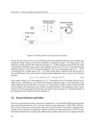


![CHAPTER 5. CORE LOSS MEASUREMENT SYSTEM
System error Way to detect
Desired signal frequency outside al-
lowed range
User enters frequency value greater than 200 kHz or smaller than
1 kHz for high frequency excitation and higher than 1 kHz or
lower than 50 Hz for sinusoidal excitation
Desired temperature outside allowed
range
User enters desired core temperature value that is higher than
160◦C or a positive value lower than 30◦C
Average current too high Reference value of the average current to be written to the DSP
is greater than 25 A
DC link voltage too high DC link voltage that should be set is higher than 450 V for high
frequency excitation and 300 V for sinusoidal excitation
DC link voltage too low DC link voltage that should be set is lower than 3 V
DC link in current limitation mode Measured current of the DC power supply is equal to 1.7 A
Unknown error There is no voltage or current on the CUT when the program
expects that excitation signal should exist
Table 5.8: List of errors that the software can detect with short explanation on how they are detected.
When the system is brought to the desired operating point, measurements can be taken. Before taking the
measurements, the oscilloscope has to be set. In the single operation mode, the user can set the oscilloscope
manually, or the settings can be made automatically. The button Set oscilloscope automatically is connected
to the function that does the setting. Since the losses are calculated through the integration of the BH curve,
current and voltage measurements have to be taken for exactly one period or for a time interval that is equal
to integer multiple of the signal period. Therefore, for signals that have frequencies lower than 10 kHz,
horizontal oscilloscope resolution is set so that exactly one period is visible in the oscilloscope screen. For
higher frequencies, horizontal resolution is set so that 10 full periods are visible on the oscilloscope screen.
The oscilloscope has a limited set of scales for setting the horizontal axes. Therefore, the set of frequencies
for which the automatic oscilloscope setting is possible is also limited. Table 5.9 lists frequency values for
which the automatic setting is possible. The oscilloscope vertical settings are set so that the best possible
f [kHz]
High frequency excitation 1 2 5 10 20 50 100 200
Sinusoidal excitation 0.05 0.1 0.2 0.5
Table 5.9: List of frequencies for which the automatic oscilloscope setting is possible.
resolution is obtained while still having the whole signals visible on the oscilloscope screen.
Button Get results is used for taking the measurement and calculating core losses. The function that
is connected to this button takes the current and voltage measurement from the oscilloscope and delays
measured current in order to compensate for the deskew time. Losses per unit volume are then calculated
according to the equations 5.1, 5.2 and 5.3. This is repeated three times and the actual core loss value is
taken as a mean value. Upon taking the measurements, the results box is populated with the values that
were actually measured. Measured voltage and current, as well as the calculated flux density, magnetic field
strength and core loss are stored to a temporary Matlab file. The results can then be saved permanently by
the user. In case the data is not saved, the temporary file will be overwritten after the next measurement.
56](https://image.slidesharecdn.com/b2c598c0-acc4-4f16-a555-962d4c8820c3-160325211659/85/Final_report-70-320.jpg)


![CHAPTER 6. CORE LOSS MEASUREMENT DATABASE
- 1 5 0 - 1 0 0 - 5 0 0 5 0 1 0 0
- 0 . 4
- 0 . 3
- 0 . 2
- 0 . 1
0
0 . 1
0 . 2
0 . 3
0 . 4
H [ A / m ]
B[T]
N 8 7
B H c u r v e f= 5 0 0 H z T = 6 0 ° C
in it ia l B H r e la t io n f= 5 0 0 H z T = 6 0 ° C
1 0
- 1
1 0
0
1 0
3
1 0
4
1 0
5
1 0
6
B
p p
[ T ]
P
v
[W/m3]
N 8 7
f= 5 k H z H D C = 0 A / m T = 2 3 ° C
f= 2 0 k H z H D C = 0 A / m T = 2 3 ° C
f= 5 0 k H z H D C = 0 A / m T = 2 3 ° C
2 0 3 0 4 0 5 0 6 0 7 0 8 0 9 0 1 0 0 1 1 0 1 2 0
1 0
3
1 0
4
1 0
5
T [ ° C ]
P
v
[W/m3]
N 8 7
f= 5 k H z B p p = 0 . 2 T H D C = 0 A / m
f= 2 0 k H z B p p = 0 . 2 T H D C = 0 A / m
f= 5 0 k H z B p p = 0 . 2 T H D C = 0 A / m
0 1 2 3 4 5 6 7 8
0 . 2 0 3 5
0 . 2 0 4
0 . 2 0 4 5
0 . 2 0 5
0 . 2 0 5 5
0 . 2 0 6
0 . 2 0 6 5
0 . 2 0 7
0 . 2 0 7 5
0 . 2 0 8
t
1
[ u s ]
E[J]
N 8 7
B p p = 0 . 1 T t 2 = 2 5 u s T = 2 3 ° C
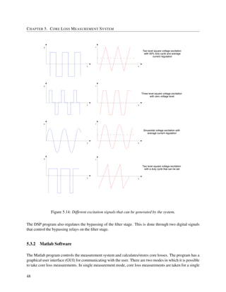
Figure 6.4: Examples of some plots made for N87 ferrite material from EPCOS. Top left plot shows the BH
curve of the material; top right shows core losses as a function of peak-to-peak flux density ripple for
different signal frequency values; bottom left shows core loss as a function of temperature at different
signal frequencies; bottom right shows dependence of loss energy from zero voltage time in a sweep
measurement done with three level voltage excitation.
70](https://image.slidesharecdn.com/b2c598c0-acc4-4f16-a555-962d4c8820c3-160325211659/85/Final_report-84-320.jpg)
![Chapter 7
Magnetic Component Design Software
The magnetic component design software already existed before the start of this master thesis project. In
this project it has been connected to the core loss measurement database in order to complete the design
environment. Also the software was slightly improved by adding the relaxation loss model that did not
exist before. This chapter gives a short overview of the design software and describes the extensions of the
software in detail.
The magnetic component design software can be used for calculating core losses for four different core
geometries. The hybrid core loss model described in Chapter 3 is used. Also, winding loss calculation for
solid wire is possible, with the prospect of extending the software so that calculation would be possible for
litz wire or foil windings. Winding losses are calculated by using the models for skin effect and proximity
effect losses. In addition, based on the calculated losses, the software can calculate expected temperature
for both the core and the windings. The software is also capable of calculating inductance values for four
implemented core geometries. Excitation signals for which losses and temperature can be calculated can be
selected from a list of predefined signal waveforms (where square, sinusoidal and trapezoidal flux density
waveforms are available) or they can be imported from circuit simulation software such as Simplorer or
Matlab. Figure 7.1 shows how the graphical user interface of the design software looks like. Detailed
description of the design software can be found in [32].
7.1 Software Extensions
Magnetic component design software has been extended so that it can use the data from the database as a
loss map. In order to form the loss map, the loss measurements from the database are fused together into a
hyper-matrix. This is done by using methods of the class for interacting with the database. Used methods are
listed in Appendix F. The software also uses the information on the initial permeability of the material that
is stored in the database. In addition, initial BH relation that the software needs for inductance calculation
is extracted from one of the material BH curves stored in the database. Although, such an approximation of
the initial BH relation is not very accurate in the area where the strength of magnetic field is close to zero,
it is the best approximation that can be made from a dynamic BH loop measurement. This is necessary for
materials for which manufacturers do not provide the initial relation data. Initial BH relation is calculated
by assigning to each H value, the mean of the two B values that correspond to it in the BH curve. Figure
71](https://image.slidesharecdn.com/b2c598c0-acc4-4f16-a555-962d4c8820c3-160325211659/85/Final_report-85-320.jpg)

![CHAPTER 7. MAGNETIC COMPONENT DESIGN SOFTWARE
- 1 5 0 - 1 0 0 - 5 0 0 5 0 1 0 0 1 5 0
- 0 . 4
- 0 . 3
- 0 . 2
- 0 . 1
0
0 . 1
0 . 2
0 . 3
0 . 4
H [ A / m ]
B[T]
N 8 7
M a t e r ia l B H c u r v e
E x t r a c t e d in it ia l B H r e la t io n
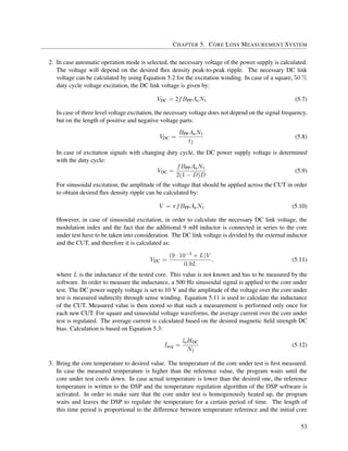
Figure 7.2: BH curve for EPCOS N87 ferrite with initial BH relation extracted from the curve.
For a particular sweep operating point defined by the flux density peak-to-peak ripple (BPP) and time length
of positive and negative voltage period (t2), this equation becomes:
∆E = kr
BPP
t2
αr
(Bpp)βr
(7.3)
The value for ∆E can be calculated from the measurement data by subtracting the measured energy for
t1 = 0 from energy measured for biggest t1 in the sweep measurement. Figure 7.3 illustrates the way to
calculate ∆E. By forming equation 7.3 for three different operating points, a system of three nonlinear
equations with three unknown parameters is formed. The relaxation loss model parameters are obtained by
solving this system and by using Equation 7.1 for calculating τ.
The parameter qr can be extracted from the sweep measurement data obtained with two level voltage
excitation with variable duty cycle. This parameter is used to correct the error occurring when the core
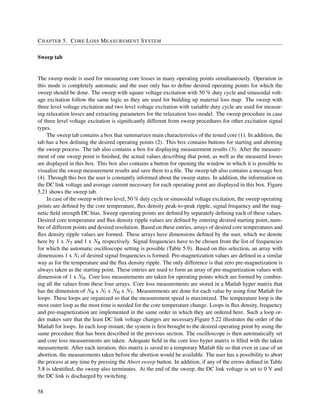
losses are calculated by only using the iGSE for low duty cycle values. If we denote the core loss calculated
by only using the iGSE, for a given duty cycle value from the sweep by PiGSE(D), we will see that for low
duty cycle values actually measured results are higher than the calculated values. On the other hand, the
measured losses are always lower than the upper loss limit given by the equation:
Pmax(D) = PiGSE(D) + Pr, (7.4)
where Pr represents the contribution of the relaxation loss, given by Equation 3.6. According to the i2
GSE
model, core losses for a given duty cycle are calculated by the following equation:
P(D) = PiGSE(D) + e−qr
D
1−D Pr (7.5)
73](https://image.slidesharecdn.com/b2c598c0-acc4-4f16-a555-962d4c8820c3-160325211659/85/Final_report-87-320.jpg)
![CHAPTER 7. MAGNETIC COMPONENT DESIGN SOFTWARE
0 10 20 30 40 50 60
0
1
2
3
4
5
6
7
t
1
[µs]
E[µJ]
∆B = 50mT, t
2
= 10µs
∆B = 100mT, t
2
= 10µs
∆B = 100mT, t2
= 5µs
τ
2∆E.
Figure 7.3: Dependence of measured sweep energy from zero voltage time period with illustration on how
to calculate ∆E. Shown measurement results are for N87 EPCOS material.
Therefore, the parameter qr has to be determined so that the losses calculated by Equation 7.5 match the
actually obtained measurement results. This can be done by finding qr that minimizes cumulative core loss
prediction error for all duty cycle values in the sweep measurement:
qr = arg max
qr
D
PiGSE(D) + e−qr
D
1−D Pr − Pmes(D) , (7.6)
where Pmes(D) represents the measured sweep point for a given duty cycle. Figure 7.4 illustrates the dif-
ference between actually measured values and the loss calculation in case of only using the iGSE and in
case when the i2
GSE with properly determined qr is used for the loss calculation. The program calculates
PiGSE(D) by extracting ki, α and β from the material loss map for each duty cycle point in the sweep.
74](https://image.slidesharecdn.com/b2c598c0-acc4-4f16-a555-962d4c8820c3-160325211659/85/Final_report-88-320.jpg)
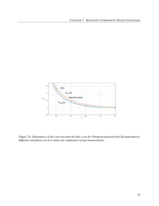

![Chapter 8
Design Environment Usage Illustration and
Validation
In order to demonstrate how the built design environment can be used for magnetic component design, a full
design procedure is illustrated on a real example. A design procedure in which the environment is used is
compared with a more traditional design approach in order to stress all the advantages of using the design
environment. In addition, loss and temperature measurements were done for some of the designed inductors
in order to validate the models used by the design environment. This chapter first describes the design
procedure which makes the full use of the environment and compares this procedure with a more classical
design approach. The design procedure is than illustrated on a design example. At the end, experiments and
measurements done with the built components in order to validate the modeling accuracy of the environment
are described.
8.1 Design Procedure
Designing inductors and transformers can often be a big challenge. The main problem lies in the accurate
prediction of component loss and temperature. The actual design procedure may vary depending on the
application, but also on engineers experience and preference. Typical inductor design involves a lot of
generally known rules of thumb, but also a lot of design rules that engineers develop themselves during
years of experience. In this section a typical inductor design procedure is described. This procedure is then
used to highlight all the improvements that the built design environment brings into the design process.
One typical inductor design procedure is described in [33]. It is based on many years of experience that
the author has in designing magnetic components. Although slight variations of the procedure are possible
among engineers, it is reasonable to assume that this design approach well illustrates the most common
strategy used by engineers in designing magnetic components. In this procedure, component inductance and
peak current value have to be determined first. Based on this, the design engineer has to decide on the shape
and size of the used core. Also, a suitable core material should be selected. Good knowledge on properties
of different magnetic materials can greatly help in this selection. Initial selection of the core size and shape
is not straightforward and mainly depends on the design engineer experience and feeling. Depending on the
77](https://image.slidesharecdn.com/b2c598c0-acc4-4f16-a555-962d4c8820c3-160325211659/85/Final_report-91-320.jpg)

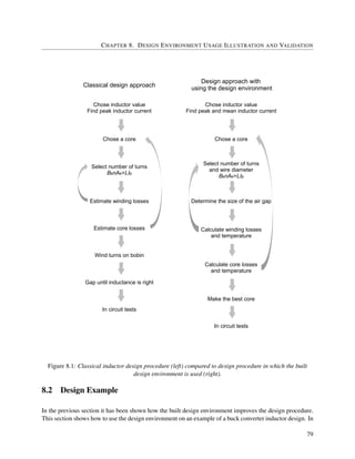


![CHAPTER 8. DESIGN ENVIRONMENT USAGE ILLUSTRATION AND VALIDATION
Inductor
label
Used core
Air gap
[mm]
Winding
no.
Wire
diameter
[mm]
Max. di-
mension
[mm]
Loss [W]
Max.
tempera-
ture
[◦C]
L1 E25137 1.05 27 0.45 25 1.36 77.7
L2 E25137 1.05 27 0.63 25 1 65
L3 E25137 1.05 27 0.8 25 1.15 67.4
L7 E30157 1 26 0.45 30 1.15 67
L7 E30157 1 26 0.63 30 0.84 58.9
L7 E30157 1 26 0.8 30 0.7 50.9
L13 E32169 0.55 18 0.45 32 0.76 47
L13 E32169 0.55 18 0.63 32 0.56 39.8
L13 E32169 0.55 18 0.8 32 0.5 37.6
Table 8.2: List of possible buck converter inductors with calculated total losses and maximal temperature.
8.3 Modeling Validation
In order to validate loss and thermal models used by the design environment and to check its overall accuracy,
inductors labeled as L3, L8 and L15 in Table 8.2 were built. Built inductors were used in the actual buck
converter and their core and winding losses and temperatures were measured and compared to the values
calculated by the magnetic component design software. Measurements were done for two operating modes
of the buck converter. First mode was the continuous conduction mode, with the same specifications as the
ones for which the inductor was designed (Table 8.1). Measurements were also done in the discontinuous
conduction mode of the buck converter. In this case, the output power was decreased to 48 W, and the
output voltage was increased to 20 V. Resulting current waveforms over the inductor are shown in Figure
8.3. Losses have been measured with the Power Analyzer Yokogawa WT3000, which calculates the real
power by measuring voltage and current. Core and winding temperatures have been measured with infrared
camera FLIR ThermaCAM. Tables 8.3 and 8.4 give the comparison between predicted and measured loss
and temperature values for continuous and discontinuous conduction mode respectively. Pictures made with
the infra red camera during the measurements are also shown.
82](https://image.slidesharecdn.com/b2c598c0-acc4-4f16-a555-962d4c8820c3-160325211659/85/Final_report-96-320.jpg)
![CHAPTER 8. DESIGN ENVIRONMENT USAGE ILLUSTRATION AND VALIDATION
L3 = 44.7 μH
Calculated Measured Rel. error
Loss [W]
core: 0.13
1.26 8.73%winding: 1.02
total: 1.15
Core
temperature 38◦
C 40◦
C 5%
Winding
temperature 67◦
C 68◦
C 1.5%
L8 = 47.7 μH
Calculated Measured Rel. error
Loss [W]
core: 0.16
0.9 6.67%winding: 0.68
total: 0.84
Core
temperature 35.4◦
C 35◦
C 1.14%
Winding
temperature 58.9◦
C 63◦
C 6.5%
L15 = 45.8 μH
Calculated Measured Rel. error
Loss [W]
core: 0.25
0.53 5.66%winding: 0.25
total: 0.50
Core
temperature 35.8◦
C 34◦
C 5.29%
Winding
temperature 37.6◦
C 41◦
C 8.29%
Table 8.3: Comparison of the measurement results and the values calculated with the magnetic component
design software for the continuous conduction mode.
83](https://image.slidesharecdn.com/b2c598c0-acc4-4f16-a555-962d4c8820c3-160325211659/85/Final_report-97-320.jpg)
![CHAPTER 8. DESIGN ENVIRONMENT USAGE ILLUSTRATION AND VALIDATION
L3 = 44.7 μH
Calculated Measured Rel. error
Loss [W]
core: 0.12
0.64 1.56%winding: 0.51
total: 0.63
Core
temperature 39.2◦
C 38◦
C 3.16%
Winding
temperature 49.9◦
C 48◦
C 3.96%
L8 = 47.7 μH
Calculated Measured Rel. error
Loss [W]
core: 0.1
0.62 4.84%winding: 0.49
total: 0.59
Core
temperature 33.3◦
C 33◦
C 0.9%
Winding
temperature 47.9◦
C 48◦
C 0.2%
L15 = 45.8 μH
Calculated Measured Rel. error
Loss [W]
core: 0.18
0.43 9.3%winding: 0.21
total: 0.39
Core
temperature 33.8◦
C 32◦
C 5.62%
Winding
temperature 35.7◦
C 38◦
C 6.06%
Table 8.4: Comparison of the the measurement results and the values calculated with the magnetic
component design software for discontinuous conduction mode.
84](https://image.slidesharecdn.com/b2c598c0-acc4-4f16-a555-962d4c8820c3-160325211659/85/Final_report-98-320.jpg)
![CHAPTER 8. DESIGN ENVIRONMENT USAGE ILLUSTRATION AND VALIDATION
0 1 0 2 0 3 0 4 0 5 0 6 0 7 0
0
1
2
3
4
5
6
7
8
t [ µ s ]
i
L
[A]
In d u c t o r c u r re n t in c o n t in u o u s c o n d u c t io n m o d e
0 1 0 2 0 3 0 4 0 5 0 6 0 7 0
0
1
2
3
4
5
6
7
8
t [ µ s ]
iL
[A]
In d u c t o r c u r r e n t in d is c o n t in u o u s c o n d u c t io n m o d e
t [μs] t [μs]
Inductor current in continuous conduction mode Inductor current in discontinuous conduction mode
IL[A]
IL[A]
Figure 8.3: Current waveforms of tested inductors in two operational modes of the buck converter.
As can be seen from the tables, a very good accuracy is achieved. For all the calculated loss and
temperature values, a relative error less than 10 % is achieved. This is very good accuracy when having in
mind that all the calculations were completely based on the approximated initial BH relation. Therefore, due
to errors in this approximation, there are errors in the calculated inductance. Actually measured inductance
values are shown in Tables 8.3 and 8.4. During the measurements on the buck converter, the inductor current
was not exactly regulated, only the output power and voltage were set to exactly match the specifications.
Therefore, any errors in the inductance influence the actual shape of the inductor current and consequently
the measured losses.
In addition to measurements done with the buck converter circuitry, more measurements were performed
with these three inductors. One more inductor was built for the purpose of verifying loss and temperature
calculations. Additional measurements with these four cores were done by using the core loss measurement
system for generating triangular current excitations at different frequencies. In all these measurements a
relative error less than 10 % was observed. These additional measurements are documented in Appendix H.
One interesting thing to consider when talking about modeling accuracy is what effect the improved core
loss model on the overall loss calculation accuracy have. This analysis can go into two directions. First
one is to analyze what is the contribution of having the loss map and considering the influence that the pre-
magnetization and temperature have on core losses. Second one is to analyze the impact of taking relaxation
loss into account. In order to determine this, two experiments were done. In the first one, losses in case
of the continuous conduction mode were recalculated with not taking the pre-magnetization into account.
This was done by simply setting the HDC value in the software to zero (this also reduces the winding losses,
however, it has been shown that this effect is negligible). The relative error for all three inductors in this
case was compared to the error in case of normal loss calculation. In the second experiment, losses in case
of continuous conduction mode were recalculated with not considering relaxation losses. This was done by
artificially setting the relaxation loss model parameters to zero in the software. Again, the relative errors
were compared with the case of having the normal loss calculation. Figure 8.4 shows the comparison of
relative errors for these two experiments. As can be seen, not taking the influence of pre-magnetization into
85](https://image.slidesharecdn.com/b2c598c0-acc4-4f16-a555-962d4c8820c3-160325211659/85/Final_report-99-320.jpg)


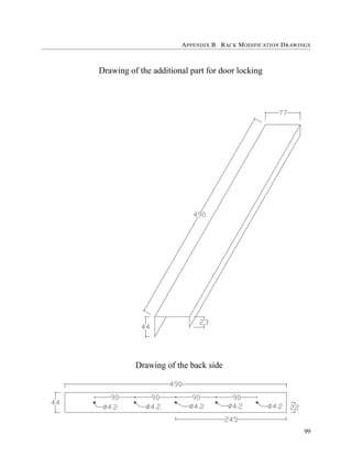


![Appendix E
Core Loss Measurement System Software
Functions
This section gives the list of all the functions that make up the software for controlling the core loss mea-
surement system. For each of the functions, a short description of its function is given.
• additional plots ( )
Function used for making additional plots in the sweep measurement.
• [ JperV, H, B ] = BHAnalyse ( N1, N2, A, MLP, t, u, i )
Function for calculating loss energy per unit volume, magnetic field strength and flux density out of
measured voltage and current and based on the data describing the CUT.
• [ alfar, betar, kr ] = calculate relaxation parameters ( data )
Function for calculating some of the relaxation loss model parameters based on the sweep measure-
ments done with three level voltage excitation.
• [ alfa, beta, ki ] = calculate steinmetz parameters ( f, dB, loss, type )
Function for calculating the Steinmetz parameters for the sweep done with sinusoidal voltage exci-
tation or the generalized Steinmetz parameters for the sweep done with two level voltage excitation
with 50 % duty cycle.
• com init ( )
Function used for opening the serial port and creating a global variable for communication with the
DSP.
• [ currentOFFSET ] = curOFFSET ( )
Function for determining the zero offset of the current measurement.
• [ signal SH ] = deskew ( signal, t, shift )
Function for deskewing the given current signal for the specified amount of shift time.
• [ value, err ] = dsp read ( var, format, addindex )
Function for reading the specified DSP variable value.
113](https://image.slidesharecdn.com/b2c598c0-acc4-4f16-a555-962d4c8820c3-160325211659/85/Final_report-127-320.jpg)
![APPENDIX E. CORE LOSS MEASUREMENT SYSTEM SOFTWARE FUNCTIONS
• [ err ] = dsp reset ( )
Function for resetting the DSP.
• [ err ] = dsp write ( var, value, format, addindex )
Function for writing a value to the specified DSP variable.
• [ L ] = getinductance2 ( Nprim, Nsec, AperDiv )
Function that measures the CUT inductance.
• [ u, i, t, ack ] = getOSC ( )
Function that reads the CUT secondary side voltage and primary side current from the oscilloscope.
• [ out ] = is current saturated ( in )
Function that identifies whether the DC power supply is in current limit operation mode.
• [ abort ] = mode2on ( )
Function that sets the DSP mode variable to 2 (two level voltage excitation with 50 % duty cycle) and
monitors the DSP operation until the measured current reaches the desired reference value.
• [ abort ] = mode5on ( )
Function that sets the DSP mode variable to 5 (sinusoidal voltage excitation) and monitors the DSP
operation until the measured current reaches the desired reference value.
• [ temp ] = read core temp ( )
Function that reads the number representing the core temperature measured by the temperature sensor
and converts it to ◦C.
• [ out ] = readmapfile ( )
Function used for reading the map file necessary for the communication with the DSP.
• [ curr , vol ] = readPowerSupply ( num )
Function for reading the actual current and voltage of the DC power supply.
• [ ack ] = scaleOSC ( signal )
Function for auto scaling of the oscilloscope.
• [ ack ] = set ref temp ( temp )
Function for writing the desired core under test reference temperature to the DSP.
• [ ack, v ] = setBpp ( dB, Nprim, Nsec, cross section, MLP, v, signal )
Function for fine regulation of the flux density peak-to-peak ripple.
• [ ack ] = setosc ( i avg, f, Nprim, Nsec, AperDiv, v1, all )
Function for setting the oscilloscope horizontal and vertical axis scale.
• [ ack ] = setPowerSupply ( v, imax, out )
Function for setting the desired DC power supply voltage.
• [ ack ] = setTemp ( Temperature, code )
Function that sets the desired CUT temperature and monitors the DSP operation until the reference
temperature is reached.
114](https://image.slidesharecdn.com/b2c598c0-acc4-4f16-a555-962d4c8820c3-160325211659/85/Final_report-128-320.jpg)


![Appendix F
Database Management Software Functions
Software for database management and data visualization is organized in a single Matlab class which is
used for communicating with the database. This section lists all the methods of this class and gives a short
description for each one.
• [ obj ] = database1 ( )
Class constructor, it initializes the communication with the database.
• [ obj output ] = core materials ( obj )
Method that returns the list of all the materials that are stored in the database.
• [ obj ] = add material ( obj, material, manufacturer, init perm, sat flux dens, el conduc, ther conduc )
Method for adding a new material to the database.
• [ properties ] = return material properties ( obj, material )
This method returns material properties that are stored in the database for the given material.
• [ date ] = return date ( obj, material )
Method that returns the date and time of the last measurement stored in the database for the given
material.
• [ obj ] = include file ( obj, file location, filename, j )
Method that adds new measurement data from a saved file to the database.
• [ out ] = is in database ( obj, material, manufacturer )
Method that checks whether the given material is stored in the database.
• [ out ] = take data ( obj, material )
Method that returns all the data stored in the database for a given material, data is returned in a form
of Matlab structure.
• [ obj, out ] = getBH ( obj, material )
This method collects and returns all the scanned BH curves that are stored in the database for the
given material.
117](https://image.slidesharecdn.com/b2c598c0-acc4-4f16-a555-962d4c8820c3-160325211659/85/Final_report-131-320.jpg)
![APPENDIX F. DATABASE MANAGEMENT SOFTWARE FUNCTIONS
• [ obj, out ] = return high frequency ( obj, material )
This method collects and returns, in a form of Matlab structure, all the sweep measurements done with
square voltage excitation with 50 % duty cycle that are stored in the database for the given material.
• [ obj, out ] = return low frequency ( obj, material )
This method collects and returns, in a form of Matlab structure, all the sweep measurements done
with sinusoidal voltage excitation that are stored in the database for the given material.
• [ obj, out ] = return relaxation losses ( obj, material )
This method collects and returns, in a form of Matlab structure, all the sweep measurements done
for the extraction of relaxation loss model parameters that are stored in the database for the given
material.
• [ obj ] = delete from database ( obj, material, manufacturer )
Method that removes the given material from the database.
• [ obj ] = close database ( obj )
Method that terminates the communication with the database.
118](https://image.slidesharecdn.com/b2c598c0-acc4-4f16-a555-962d4c8820c3-160325211659/85/Final_report-132-320.jpg)

![APPENDIX G. ON SELECTING AND PREPARING SAMPLE CORES FOR LOSS MEASUREMENTS
Frequency range [kHz] Core cross section range [mm2]
0.05 – 1 400 – 800
1 – 100 90 – 300
100 – 200 60 – 90
Table G.1: Optimal CUT cross section ranges for different excitation frequency values.
used. When building test cores out of U shaped parts, two parts should be tightly pressed together in order
to make sure that there is no air gap between them. Presence of any air gap can have significant influence
on the measurement accuracy.
120](https://image.slidesharecdn.com/b2c598c0-acc4-4f16-a555-962d4c8820c3-160325211659/85/Final_report-134-320.jpg)


![APPENDIX H. ADDITIONAL LOSS AND TEMPERATURE MEASUREMENTS
Results for inductor L3
Operating point Calculated losses Meas. losses Comparison
BPP [T] f [kHz] Core loss [W] Winding loss [W] Total loss [W] Total loss [W] Rel. error [%]
0.1 5 0.002 0.05 0.052 0.05 4
0.15 5 0.006 0.11 0.116 0.11 5.45
0.2 5 0.01 0.2 0.21 0.2 5
0.25 5 0.02 0.31 0.33 0.32 3.13
0.3 5 0.03 0.45 0.48 0.46 4.35
0.35 5 0.05 0.6 0.65 0.63 3.17
0.1 10 0.005 0.05 0.055 0.06 8.33
0.15 10 0.01 0.12 0.13 0.13 0
0.2 10 0.02 0.2 0.22 0.24 8.33
0.25 10 0.04 0.32 0.36 0.37 2.7
0.3 10 0.06 0.47 0.53 0.54 1.85
0.35 10 0.09 0.63 0.72 0.74 2.7
0.1 20 0.01 0.06 0.07 0.077 9.09
0.15 20 0.03 0.13 0.16 0.17 5.88
0.2 20 0.05 0.24 0.29 0.32 9.38
0.25 20 0.08 0.37 0.45 0.49 8.22
0.3 20 0.13 0.54 0.67 0.73 8.22
0.35 20 0.18 0.73 0.91 1 9
Table H.1: Comparison of the calculated and the measured loss values for the inductor L3 in case the
temperature modeling is not considered.
124](https://image.slidesharecdn.com/b2c598c0-acc4-4f16-a555-962d4c8820c3-160325211659/85/Final_report-138-320.jpg)

![APPENDIX H. ADDITIONAL LOSS AND TEMPERATURE MEASUREMENTS
Results for inductor L15
Operating point Calculated losses Meas. losses Comparison
BPP [T] f [kHz] Core loss [W] Winding loss [W] Total loss [W] Total loss [W] Rel. error [%]
0.1 5 0.006 0.032 0.038 0.041 7.32
0.15 5 0.017 0.07 0.087 0.083 4.82
0.2 5 0.035 0.126 0.161 0.15 7.33
0.25 5 0.056 0.2 0.256 0.25 2.4
0.3 5 0.084 0.28 0.364 0.36 1.11
0.35 5 0.12 0.386 0.506 0.5 1.2
0.1 10 0.012 0.033 0.045 0.049 8.16
0.15 10 0.031 0.075 0.106 0.1 6
0.2 10 0.06 0.13 0.19 0.18 5.55
0.25 10 0.1 0.2 0.3 0.31 3.23
0.3 10 0.16 0.3 0.46 0.44 4.55
0.35 10 0.24 0.4 0.64 0.64 0
0.1 20 0.025 0.04 0.065 0.06 8.33
0.15 20 0.06 0.09 0.15 0.156 3.85
0.2 20 0.12 0.16 0.28 0.27 3.7
0.25 20 0.2 0.25 0.45 0.43 4.65
0.3 20 0.32 0.36 0.68 0.63 7.94
0.35 20 0.48 0.49 0.97 0.89 8.99
Table H.2: Comparison of the calculated and the measured loss values for the inductor L15 in case
temperature modeling is not considered.
126](https://image.slidesharecdn.com/b2c598c0-acc4-4f16-a555-962d4c8820c3-160325211659/85/Final_report-140-320.jpg)
![APPENDIX H. ADDITIONAL LOSS AND TEMPERATURE MEASUREMENTS
Results for inductor L22
Operating point Calculated losses Meas. losses Comparison
BPP [T] f [kHz] Core loss [W] Winding loss [W] Total loss [W] Total loss [W] Rel. error [%]
0.1 5 0.0015 0.025 0.0265 0.026 1.92
0.15 5 0.004 0.057 0.061 0.058 5.17
0.2 5 0.008 0.1 0.108 0.1 8
0.25 5 0.01 0.16 0.17 0.16 6.25
0.3 5 0.02 0.23 0.25 0.23 8.69
0.35 5 0.03 0.3 0.33 0.32 3.12
0.1 10 0.003 0.027 0.03 0.029 3.45
0.15 10 0.007 0.061 0.068 0.065 4.62
0.2 10 0.014 0.109 0.123 0.12 2.5
0.25 10 0.02 0.17 0.19 0.18 5.55
0.3 10 0.04 0.25 0.29 0.27 7.4
0.35 10 0.055 0.33 0.385 0.36 6.94
0.1 20 0.006 0.035 0.041 0.04 2.5
0.15 20 0.01 0.08 0.09 0.093 3.22
0.2 20 0.03 0.14 0.17 0.17 0
0.25 20 0.05 0.22 0.27 0.27 0
0.3 20 0.07 0.32 0.39 0.38 2.63
0.35 20 0.11 0.43 0.54 0.52 3.85
Table H.3: Comparison of the calculated and the measured loss values for the inductor L3 in case
temperature modeling is not considered.
127](https://image.slidesharecdn.com/b2c598c0-acc4-4f16-a555-962d4c8820c3-160325211659/85/Final_report-141-320.jpg)
![APPENDIXH.ADDITIONALLOSSANDTEMPERATUREMEASUREMENTS
Operating point Calculated losses and temperature Meas. losses and temperature Comparison
BPP f [kHz]
Core
loss [W]
Winding
loss [W]
Total
loss [W]
Core
temp.
[◦C]
Winding
temp.
[◦C]
Core
loss [W]
Core
temp.
[◦C]
Winding
temp.
[◦C]
Relative
loss er-
ror [%]
Relative
core
temp.
er-
ror [%]
Relative
wind-
ing
temp.
er-
ror [%]
Results for inductor L3
0.3 10 0.07 0.39 0.46 36 44.3 0.5 40 49 8 10 9.59
0.3 20 0.13 0.58 0.71 40.5 52.5 0.47 43 58 4.05 5.81 9.48
0.35 20 0.18 0.8 0.98 45 61 1.01 49 66 2.97 8.16 7.57
Results for inductor L15
0.3 10 0.15 0.31 0.46 34 39 0.45 35 43 2.22 2.94 9.3
0.3 20 0.28 0.37 0.65 37.9 41.7 0.6 37 45 8.33 2.43 7.33
0.35 20 0.4 0.52 0.92 42 47.1 0.94 44 52 2.13 4.54 9.42
Results for inductor L22
0.3 10 0.035 0.24 0.275 34.2 40.6 0.27 37 42 1.86 7.49 3.33
0.3 20 0.06 0.33 0.39 37.5 45.6 0.38 39 46 2.63 3.85 0.87
0.35 20 0.09 0.45 0.54 41.4 52.1 0.52 44 52 3.85 5.9 0.19
0.4 50 0.23 1.44 1.67 64.5 97 1.6 60 91 4.38 7.5 6.59
Table H.4: Comparison of the calculated and the measured values in experiments in which the component temperature is taken into account.
128](https://image.slidesharecdn.com/b2c598c0-acc4-4f16-a555-962d4c8820c3-160325211659/85/Final_report-142-320.jpg)
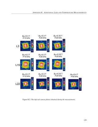

![Bibliography
[1] A.Van de Bossche, V. C. Valchev: Inductors and Transformers for Power Electronics, Taylor & Francis
Group, London, ISBN 1-57444-679-7, 2005
[2] Colonel Wm. T. McLyman: Transformer and Inductor Desigh Handbook, Marcel Dekker, Inc., New
York, ISBN 0-8247-5393-3, 2004
[3] W. Shen: Doctoral dissertation: Design of High-density Transformers for High-Frequency High-power
Converters, Virginia Polytechnic Institute and State University, Blacksburg, Virginia, July 2006
[4] 2011 Magnetics Powder Core Catalog, available online at: http://www.mag-inc.com/design/technical-
documents
[5] Micrometals catalog: Power Conversion & Line Filter Applications, Issue L, February 2007, available
online at: http://www.micrometals.com/pcparts/PC L.pdf
[6] S. M. Ni and K. T. Lwin: Production of Manganese-Zync Ferrite Cores for Electronic Applications,
World Academy of Science, Engineering and Technology, vol. 46, pp.150-155,2008
[7] M. E. McHenry, M. A. Willard, D. E. Laughlin: Amorphous and nanocrystalline materials for appli-
cations as soft magnets, Progress in Materials Science, vol. 44, pp. 291-433, 1999
[8] Magnetic Materials Producers Association: Soft Ferrites, a User’s Guide, 1998, available online at:
http://www.magneticsgroup.com/pdf/mmpa
[9] Vacuumschmelze catalog: Soft Magnetic Materials and Semi–finished Products, available online at:
http://www.vacuumschmelze.de/fileadmin/documents/broschueren/htbrosch/Pb-pht-1.pdf
[10] www.mag-inc.com
[11] www.vacuumschmelze.de
[12] www.global.tdk.com
[13] www.micrometals.com
[14] www.metglas.com/
[15] www.magnetec.de/
[16] www.epcos.com
131](https://image.slidesharecdn.com/b2c598c0-acc4-4f16-a555-962d4c8820c3-160325211659/85/Final_report-145-320.jpg)
![BIBLIOGRAPHY
[17] www.ferroxcube.com/
[18] J. Reinert, A. Brockmeyer, and R. De Doncker: Calculation of core losses in ferro- and ferrimagnetic
materials based on the modified Steinmetz equation, IEEE Transactions on Industry Applications, vol.
37, no. 4, pp. 1055-1061, 2001
[19] J. Li, T. Abdulah and C. R. Sullivan: Improved calculation of core loss with nonsinusoidal waveforms,
Industry Applications Conference, 36th IEEE IAS Anual Meeting, vol. 4, pp. 2203-2210, 2001
[20] K. Venkatachalam, C. R. Sullivan, T. Abdallah and H. Tacca: Accurate prediction of ferrite core loss
with nonsinusoidal waveforms using only steinmetz parameters, in Proc. of IEEE Workshop on Com-
puters in Power Electronics, pp. 36-41, 2002
[21] D.C. Jiles and D.L. Atherton: Theory of ferromagnetic hysteresis, Magn. Magn. Mater., vol. 61, pp.48-
60, 1986
[22] S. Y. R. Hui and J. Zhu: Magnetic hysteresis modeling and simulation using the Preisach theoty and
TLM technique, in Proc. IEEE PESC’94, pp.837-842, 1994
[23] C. P. Steinmetz: On the law of hysteresis, in Proc. IEEE, vol. 72, pp.837-842, 1984
[24] S. Iysu, K. Shimizu and and K. Ishii: A novel iron loss calculation method on power converters based
on dynamic minor loops, in Proc. of European Conference on Power Electronics and and Applications,
pp. 2016-2022, 2005
[25] J. M¨uhlethaler, J. Biela, J. W. Kolar and A. Ecklebe: Core losses under DC bias condition based on
Steinmetz parameters, in Proc. IEEE/IEEJ International Power Electronics Conference (ECCE Asia),
pp. 2430-2437, 2010
[26] T. Shimizu and K. Ishii: An iron loss calculating method for AC filter inductors used on PWM inverters,
in Proc. of 37th IEEE Power Electronics Specialists Conference (PESC), pp. 1-7, 2006
[27] K. Terashima, K. Wada, T. Schimitzu, T. Nakazava, K. Ishii and Y. Hayashi: Evaluation of the iron
loss of an inductor based on dynamic minor characteristics, in Proc. of European Conference of Power
Electronics and Applications, pp. 1-8, 2007
[28] J. M¨uhlethaler, J. Biela, J. W. Kolar and A. Ecklebe: Improved core loss calculation for magnetic com-
ponents in power electronic systems, in Proc. of Applied Power Electronics Conference and Exposition
(APEC), 2011
[29] C. R. Sullivan, J.H. Harris and E. Herbert: Core losses prediction for general PWM waveforms from a
simplified set of measurement data, in Proc. of Applied Power Electronics Conference and Exposition
(APEC), pp. 1048-1055, 2010
[30] G. Bertotti: General Properties of Power Losses in Soft Ferromagnetic Materials, IEEE Transactions
on Magnetics, vol. 24, no. 1, pp. 621-630, 1998
[31] J. M¨uhlethaler, J. W. Kolar and A. Ecklebe: Loss modeling of inductive components employed in
power electronic systems, Proceedings of the 8th international conference on power electronics –
ECCA Asia, The Shilla Jeju, Korea 2011
132](https://image.slidesharecdn.com/b2c598c0-acc4-4f16-a555-962d4c8820c3-160325211659/85/Final_report-146-320.jpg)
![BIBLIOGRAPHY
[32] R. Blattman: Modeling of circuit-simulated inductive components, Semester thesis for Power Elec-
tronic Systems Laboraratory of ETH, March 2011
[33] R. Ridley: Practical high frequency magnetics design and measurement, 26th
Annual Applied Power
Electronics Conference, Ft. Worth, TX, 2011
133](https://image.slidesharecdn.com/b2c598c0-acc4-4f16-a555-962d4c8820c3-160325211659/85/Final_report-147-320.jpg)