Lund Institute of Technology

1. IFAC PROFESSIONAL BRIEF
Computer Control: An Overview
Björn Wittenmark http://www.control.lth.se/~bjorn
Karl Johan Åström http://www.control.lth.se/~kja
Karl-Erik Årzén http://www.control.lth.se/~karlerik
Department of Automatic Control
Lund Institute of Technology
Lund, Sweden
Abstract
Computer control is entering all facets of life from home electronics to produc-
tion of different products and material. Many of the computers are embedded
and thus “hidden” for the user. In many situations it is not necessary to know
anything about computer control or real-time systems to implement a simple
controller. There are, however, many situations where the result will be much
better when the sampled-data aspects of the system are taken into consideration
when the controller is designed. Also, it is very important that the real-time as-
pects are regarded. The real-time system influences the timing in the computer
and can thus minimize latency and delays in the feedback controller.
The paper introduces different aspects of computer-controlled systems from
simple approximation of continuous time controllers to design aspects of optimal
sampled-data controllers. We also point out some of the pitfalls of computer
control and discusses the practical aspects as well as the implementation issues
of computer control.
1

2. Contents
Abstract . . . . . . . . . . . . . . . . . . . . . . . . . . . . . . . . . . . . 1
1. Introduction . . . . . . . . . . . . . . . . . . . . . . . . . . . . . . . 4
Computer-controlled Systems . . . . . . . . . . . . . . . . . . . . . . 4
The Sampling Process . . . . . . . . . . . . . . . . . . . . . . . . . . 5
Time Dependence . . . . . . . . . . . . . . . . . . . . . . . . . . . . . 5
Aliasing and New Frequencies . . . . . . . . . . . . . . . . . . . . . 6
Approximation of Continuous-time Controllers . . . . . . . . . . . . 6
Is There a Need for Special Design Methods? . . . . . . . . . . . . . 8
Summary . . . . . . . . . . . . . . . . . . . . . . . . . . . . . . . . . . 9
2. Sampling and Reconstruction . . . . . . . . . . . . . . . . . . . 11
Shannon’s Sampling Theorem . . . . . . . . . . . . . . . . . . . . . . 11
Aliasing and Antialiasing Filters . . . . . . . . . . . . . . . . . . . . 12
Zero-order Hold (ZOH) . . . . . . . . . . . . . . . . . . . . . . . . . . 13
First-order Hold . . . . . . . . . . . . . . . . . . . . . . . . . . . . . . 13
Summary . . . . . . . . . . . . . . . . . . . . . . . . . . . . . . . . . . 14
3. Mathematical Models . . . . . . . . . . . . . . . . . . . . . . . . . 15
Zero-order Hold Sampling of a Continuous-time System . . . . . . 15
First-order Hold Sampling . . . . . . . . . . . . . . . . . . . . . . . . 16
Solution of the System Equation . . . . . . . . . . . . . . . . . . . . 17
Operator Calculus and Input-output Descriptions . . . . . . . . . . 18
Z-transform . . . . . . . . . . . . . . . . . . . . . . . . . . . . . . . . 19
The Pulse-transfer Function . . . . . . . . . . . . . . . . . . . . . . . 20
Zero-order Hold Sampling . . . . . . . . . . . . . . . . . . . . . . . . 21
First-Order-Hold Sampling . . . . . . . . . . . . . . . . . . . . . . . 23
Shift-operator Calculus and Z-transforms . . . . . . . . . . . . . . . 24
Summary . . . . . . . . . . . . . . . . . . . . . . . . . . . . . . . . . . 24
4. Frequency Response . . . . . . . . . . . . . . . . . . . . . . . . . . 25
Propagation of Sinusoidal Signals . . . . . . . . . . . . . . . . . . . 25
Lifting . . . . . . . . . . . . . . . . . . . . . . . . . . . . . . . . . . . 27
Practical Consequences . . . . . . . . . . . . . . . . . . . . . . . . . 28
Summary . . . . . . . . . . . . . . . . . . . . . . . . . . . . . . . . . . 29
5. Control Design and Specifications . . . . . . . . . . . . . . . . . 30
The Process . . . . . . . . . . . . . . . . . . . . . . . . . . . . . . . . 31
Admissible Controls . . . . . . . . . . . . . . . . . . . . . . . . . . . 31
Design Parameters . . . . . . . . . . . . . . . . . . . . . . . . . . . . 31
Criteria and Specifications . . . . . . . . . . . . . . . . . . . . . . . . 32
Robustness . . . . . . . . . . . . . . . . . . . . . . . . . . . . . . . . . 32
Attenuation of Load Disturbances . . . . . . . . . . . . . . . . . . . 32
Injection of Measurement Noise . . . . . . . . . . . . . . . . . . . . 32
Command Signals Following . . . . . . . . . . . . . . . . . . . . . . 33
Summary . . . . . . . . . . . . . . . . . . . . . . . . . . . . . . . . . . 33
6. Approximation of Analog Controllers . . . . . . . . . . . . . . 34
State Model of the Controller . . . . . . . . . . . . . . . . . . . . . . 34
Transfer Functions . . . . . . . . . . . . . . . . . . . . . . . . . . . . 35
Frequency Prewarping . . . . . . . . . . . . . . . . . . . . . . . . . . 36
Step Invariance . . . . . . . . . . . . . . . . . . . . . . . . . . . . . . 37
Ramp Invariance . . . . . . . . . . . . . . . . . . . . . . . . . . . . . 38
Comparison of Approximations . . . . . . . . . . . . . . . . . . . . . 38
Selection of Sampling Interval and Antialiasing Filters . . . . . . . 39
Summary . . . . . . . . . . . . . . . . . . . . . . . . . . . . . . . . . . 40
2

3. 7. Feedforward Design . . . . . . . . . . . . . . . . . . . . . . . . . . 41
Reduction of Measurable Disturbances by Feedforward . . . . . . . 42
System Inverses . . . . . . . . . . . . . . . . . . . . . . . . . . . . . . 42
Using Feedforward to Improve Response to Command Signals . . 43
Summary . . . . . . . . . . . . . . . . . . . . . . . . . . . . . . . . . . 44
8. PID Control . . . . . . . . . . . . . . . . . . . . . . . . . . . . . . . 45
Modification of Linear Response . . . . . . . . . . . . . . . . . . . . 45
Discretization . . . . . . . . . . . . . . . . . . . . . . . . . . . . . . . 46
Incremental Algorithms . . . . . . . . . . . . . . . . . . . . . . . . . 46
Integrator Windup . . . . . . . . . . . . . . . . . . . . . . . . . . . . 47
Operational Aspects . . . . . . . . . . . . . . . . . . . . . . . . . . . 48
Computer Code . . . . . . . . . . . . . . . . . . . . . . . . . . . . . . 49
Tuning . . . . . . . . . . . . . . . . . . . . . . . . . . . . . . . . . . . 49
Summary . . . . . . . . . . . . . . . . . . . . . . . . . . . . . . . . . . 49
9. Pole-placement Design . . . . . . . . . . . . . . . . . . . . . . . . 52
The Diophantine Equation . . . . . . . . . . . . . . . . . . . . . . . . 54
Causality Conditions . . . . . . . . . . . . . . . . . . . . . . . . . . . 54
Summary of the Pole-placement Design Procedure . . . . . . . . . 54
Introduction of Integrators . . . . . . . . . . . . . . . . . . . . . . . 56
Summary . . . . . . . . . . . . . . . . . . . . . . . . . . . . . . . . . . 57
10. Optimization Based Design . . . . . . . . . . . . . . . . . . . . . 59
Linear Quadratic (LQ) Design . . . . . . . . . . . . . . . . . . . . . 59
How to Find the Weighting Matrices? . . . . . . . . . . . . . . . . . 60
Kalman Filters and LQG Control . . . . . . . . . . . . . . . . . . . . 61
H∞ Design . . . . . . . . . . . . . . . . . . . . . . . . . . . . . . . . . 62
Summary . . . . . . . . . . . . . . . . . . . . . . . . . . . . . . . . . . 64
11. Practical Issues . . . . . . . . . . . . . . . . . . . . . . . . . . . . . 65
Controller Implementation and Computational Delay . . . . . . . . 65
Controller Representation and Numerical Roundoff . . . . . . . . . 66
A-D and D-A Quantization . . . . . . . . . . . . . . . . . . . . . . . 69
Sampling Period Selection . . . . . . . . . . . . . . . . . . . . . . . . 69
Saturations and Windup . . . . . . . . . . . . . . . . . . . . . . . . . 70
Summary . . . . . . . . . . . . . . . . . . . . . . . . . . . . . . . . . . 72
12. Real-time Implementation . . . . . . . . . . . . . . . . . . . . . . 73
Real-time Systems . . . . . . . . . . . . . . . . . . . . . . . . . . . . 73
Implementation Techniques . . . . . . . . . . . . . . . . . . . . . . . 74
Concurrent Programming . . . . . . . . . . . . . . . . . . . . . . . . 75
Synchronization and Communication . . . . . . . . . . . . . . . . . 75
Periodic Controller Tasks . . . . . . . . . . . . . . . . . . . . . . . . 76
Scheduling . . . . . . . . . . . . . . . . . . . . . . . . . . . . . . . . . 79
Summary . . . . . . . . . . . . . . . . . . . . . . . . . . . . . . . . . . 81
13. Controller Timing . . . . . . . . . . . . . . . . . . . . . . . . . . . 83
Summary . . . . . . . . . . . . . . . . . . . . . . . . . . . . . . . . . . 88
14. Research Issues . . . . . . . . . . . . . . . . . . . . . . . . . . . . . 89
Acknowledgments . . . . . . . . . . . . . . . . . . . . . . . . . . . . . . 90
Notes and References . . . . . . . . . . . . . . . . . . . . . . . . . . . 91
Bibliography . . . . . . . . . . . . . . . . . . . . . . . . . . . . . . . . 91
About the Authors . . . . . . . . . . . . . . . . . . . . . . . . . . . . . 93
3

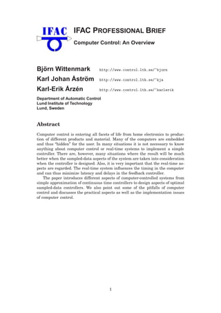
4. 1. Introduction
Computers are today essential for implementing controllers in many different
situations. The computers are often used in embedded systems. An embedded
system is a built-in computer/microprocessor that is a part of a larger system.
Many of these computers implement control functions of different physical pro-
cesses, for example, vehicles, home electronics, cellular telephones, and stand-
alone controllers. The computers are often hidden for the end-user, but it is
essential that the whole system is designed in an effective way.
Using computers has many advantages. Many problems with analog imple-
mentation can be avoided by using a computer, for instance, there are no prob-
lems with the accuracy or drift of the components. The computations are per-
formed identically day after day. It is also possible to make much more compli-
cated computations, such as iterations and solution of system of equations, using
a computer. All nonlinear, and also many linear operations, using analog tech-
nique are subject to errors, while they are much more accurately made using a
computer. Logic for alarms, start-up, and shut-down is easy to include in a com-
puter. Finally, it is possible to construct good graphical user interfaces. However,
sometimes the full advantages of the computers are not utilized. One situation
is when the computer is only used to approximately implement an analog con-
troller. The full potential of a computer-controlled system is only obtained when
also the design process is regarded from a sampled-data point of view. The the-
ory presented in this paper is essentially for linear deterministic systems. Even
if the control algorithms give the same result for identical input data the per-
formance of the closed-loop system crucially depends on the timing given by the
real-time operating system. This paper gives a brief review of some of the tools
that are important for understanding, analyzing, designing, and implementing
sampled-data control systems.
Computer-controlled Systems
A schematic diagram of a computer-controlled system is shown in Figure 1. The
system consists of
• Process
• Sampler together with Analog-to-Digital (A-D) converter
• Digital-to-Analog (D-A) converter with a hold circuit
• Computer with a clock, software for real-time applications, and control
algorithms
• Communication network
The process is a continuous-time physical system to be controlled. The input
and the output of the process are continuous-time signals. The A-D converter is
converting the analog output signal of the process into a finite precision digital
number depending on how many bits or levels that are used in the conversion.
The conversion is also quantized in time determined by the clock. This is called
the sampling process. The control algorithm thus receives data that are quan-
tized both in time and in level. The control algorithm consists of a computer
program that transforms the measurements into a desired control signal. The
control signal is transfered to the D-A converter, which with finite precision con-
verts the number in the computer into a continuous-time signal. This implies
that the D-A converter contains both a conversion unit and a hold unit that
4

5. uk
uk
k
y
k
y
Communication network
Computer
Process
y(t)
.. .. .
u(t)
t
.
and
D−A
Hold
Sampler
A−D
and
y(t)u(t)
. .. .
t
. .
.. .. ..
t
t
Figure 1 Schematic diagram of a computer-controlled system.
translates a number into a physical variable that is applied to the process. The
communication between the process, or more accurately the A-D and D-A con-
verters, and the computer is done over a communication link or network. All the
activities in the computer-controlled system are controlled by the clock with the
requirement that all the computations have to be performed within a given time.
In a distributed system there are several clocks that have to be synchronized.
The total system is thus a real-time system with hard time constraints.
The system in Figure 1 contains a continuous-time part and a sampled-data
part. It is this mixture of different classes of signals that causes some of the prob-
lems and confusion when discussing computer-controlled systems. The problem
is even more pronounced when using decentralized control where the control
system is shared between several computers. Many of the problems are avoided
if only considering the sampled-data part of the system. It is, however, impor-
tant to understand where the difficulties arise and how to avoid some of these
problems.
The Sampling Process
The times when the measured physical variables are converted into digital form
are called the sampling instants. The time between two sampling instants is the
sampling period and is denoted h. Periodic sampling is normally used, implying
that the sampling period is constant, i.e. the output is measured and the control
signal is applied each hth time unit. The sampling frequency is ωs = 2π/h.
In larger plants it may also be necessary to have control loops with different
sampling periods, giving rise to multi-rate sampling or multi-rate systems.
Time Dependence
The mixture of continuous-time and discrete-time signals makes the sampled-
data systems time dependent. This can be understood from Figure 1. Assume
that there is a disturbance added at the output of the process. Time invariance
implies that a shift of the input signal to the system should result in a similar
shift in the response of the system. Since the A-D conversion is governed by a
clock the system will react differently when the disturbance is shifted in time.
The system will, however, remain time independent provided that all changes
5

6. 0 5 10
−1
0
1
Time
Figure 2 Two signals with different frequencies, 0.1 Hz (dashed) and 0.9 Hz (full), have
the same values at all sampling instants (dots) when h = 1.
in the system, inputs and disturbances, are synchronized with the sampling
instants.
Aliasing and New Frequencies
The A-D and D-A converters are the interface between the continuous-time re-
ality and the digital world inside the computer. A natural question to ask is: Do
we loose any information by sampling a continuous-time signal?
EXAMPLE 1—ALIASING
Consider the two sinusoidal signals sin((1.8t − 1)π) and sin 0.2πt shown in Fig-
ure 2. The sampling of these signals with the sampling period h = 1 is shown
with the dots in the figure. From the sampled values there is thus no possibil-
ity to distinguish between the two signals. It is not possible to determine if the
sampled values are obtained from a low frequency signal or a high frequency sig-
nal. This implies that the continuous-time signal cannot be recovered from the
sampled-data signal, i.e. information is lost through the sampling procedure.
The sampling procedure does not only introduce loss of information but may also
introduce new frequencies. The new frequencies are due to interference between
the sampled continuous-time signal and the sampling frequency ωs = 2π/h. The
interference can introduce fading or beating in the sampled-data signal.
Approximation of Continuous-time Controllers
One way to design a sampled-data control system is to make a continuous-
time design and then make a discrete-time approximation of this controller. The
computer-controlled system should now behave as the continuous-time system
provided the sampling period is sufficiently small. An example is used to illus-
trate this procedure.
EXAMPLE 2—DISK-DRIVE POSITIONING SYSTEM
A disk-drive positioning system will be used throughout the paper to illustrate
different concepts. A schematic diagram is shown in Figure 3. Neglecting reso-
u yuc
Controller Amplifier Arm
Figure 3 A system for controlling the position of the arm of a disk drive.
6

7. 0 5 10
0
1
Output
0 5 10
−0.5
0
0.5
Input
Time (ω
0
t)
Figure 4 The step response when simulating the disk arm servo with the analog con-
troller (2) (dashed/red) and sampled-data controller (3) (solid/blue). The design param-
eter is ω0 = 1 and the sampling period is h = 0.3.
nances the dynamics relating the position y of the arm to the voltage u of the
drive amplifier is approximately described by a double integrator process
G(s) =
k
Js2
(1)
where k is the gain in the amplifier and J is the moment of inertia of the arm.
The purpose of the control system is to control the position of the arm so that
the head follows a given track and that it can be rapidly moved to a different
track. Let uc be the command signal and denote Laplace transforms with capital
letters. A simple continuous-time servo controller can be described by
U(s) =
bK
a
Uc(s) − K
s + b
s + a
Y(s) (2)
This controller is a two-degrees-of-freedom controller. Choosing the controller
parameters as
a = 2ω0
b = ω0/2
K =
2Jω2
0
k
gives a closed system with the characteristic polynomial
P(s) = (s2
+ ω0s + ω2
0)(s + ω0) = s3
+ 2ω0s2
+ 2ω2
0s + ω3
0
where the parameter ω0 is used to determine the speed of the closed-loop sys-
tem. The step response when controlling the process with the continuous-time
controller (2) is shown as the dashed line in Figure 4. The control law given by
(2) can be written as
U(s) =
bK
a
Uc(s) − KY(s) + K
a − b
s + a
Y(s) = K
b
a
Uc(s) − Y(s) + X (s)
7

8. or in the time-domain as
u(t) = K
b
a
uc(t) − y(t) + x(t)
dx(t)
dt
= −ax(t) + (a − b)y(t)
The first of these equations can be implemented directly on a computer. To find
an algorithm for the second equation the derivative dx/dt at time kh is approx-
imated with a forward difference. This gives
x(kh + h) − x(kh)
h
= −ax(kh) + (a − b)y(kh)
The following approximation of the continuous algorithm (2) is then obtained:
u(kh) = K
b
a
uc(kh) − y(kh) + x(kh)
x(kh + h) = x(kh) + h (a − b)y(kh) − ax(kh)
(3)
where y(kh) is the sampled output, u(kh) is the signal sent to the D-A converter,
and x(kh) is the internal state of the controller. This difference equation is up-
dated at each sampling instant. Since the approximation of the derivative by a
difference is good if the interval h is small, we can expect the behavior of the
computer-controlled system to be close to the continuous-time system. Figure 4
shows the arm position and the control signal for the system when ω0 = 1 and
h = 0.3. Notice that the control signal for the computer-controlled system is con-
stant between the sampling instants due to the hold circuit in the D-A converter.
Also notice that the difference between the outputs of the two simulations is very
small. The difference in the outputs is negligible if h is less than 0.1/ω0.
The computer-controlled system has slightly higher overshoot and the settling
time is a little longer. The difference between the systems decreases when the
sampling period decreases. When the sampling period increases the computer-
controlled system will, however, deteriorate and the closed-loop system becomes
unstable for long sampling periods.
The example shows that it is straightforward to obtain an algorithm for com-
puter control simply by writing the continuous-time control law as a differential
equation and approximating the derivatives by differences. The example also
indicates that the procedure seems to work well if the sampling period is suffi-
ciently small. The overshoot and the settling time are, however, a little larger
for the computer-controlled system, i.e. there is a deterioration due to the ap-
proximation.
Is There a Need for Special Design Methods?
The approximation of a continuous-time controller discussed above shows that it
is possible to derive a discrete-time controller based on continuous-time design.
There are many different approximations methods that can be used. Normally,
they are crucially dependent on choosing fairly short sampling periods. The ap-
proximation methods are possible to use also for nonlinear continuous-time con-
trollers. Deriving a sampled-data description of the process makes it possible to
utilize the full potential of a sampled-data systems and to derive other classes
8

9. 0 5 10
0
1
Position
0 5 10
0
0.5
Velocity
0 5 10
−0.5
0
0.5
Input
Time (ω
0
t)
Figure 5 The step response when simulating the disk arm servo using the analog con-
troller (3) (dashed/red) and the deadbeat controller (solid/blue). The sampling period is
h = 1.4.
of controllers that are not possible to use in continuous-time. The sampled-data
theory is also needed to explain the inter-sample and periodic behavior of the
sampled-data systems. Notice that the theory for sampled-data systems is de-
rived mainly for linear systems.
EXAMPLE 3—DEADBEAT CONTROL
Consider the disk drive in the previous example. Using a sampling interval of
h = 1.4 with ω0 = 1 gives an unstable closed-loop system if the controller (3) is
used. However, designing a discrete-time controller with the same structure as
(3) gives the performance shown in Figure 5 when h = 1.4. The controller can
be written as
u(kh) = t0uc(kh) + t1uc(kh − h) − s0 y(kh) − s1 y(kh − h) − r1u(kh − h)
where the coefficients now are chosen such that the output of the system will
reach the reference value after two samples. This is called a deadbeat controller
and it has not a continuous-time counterpart. The design parameter of the dead-
beat controller is the sampling period h, which here is chosen such that the max-
imum control signal is the same when the continuous-time and the sampled-data
controllers are used.
Summary
The examples in this chapter clearly show that there are some important issues
that are specific for sampled-data systems.
• Sampling makes the system time-varying.
9

10. • Information may be lost through sampling.
• Sampled controller have behaviors that are not achievable with continuous-
time controllers.
This requires an understanding of the interplay between the continuous-time sig-
nals and the discrete-time signals. The rest of the paper gives a brief overview of
some of the tools that are important for the analysis, design, and implementation
of sampled-data control system.
10

11. 2. Sampling and Reconstruction
A sampler is a device, driven by the clock in the system, that is converting a
continuous-time signal into a sequence of numbers. Normally, the sampler is
combined into the A-D converter, which also quantizes the sequence of numbers
into a finite, although it may be a high, precision number that is then stored in
the computer. Typically the A-D converter has 8–16 bits resolution giving 28–
216 levels of quantization. This is normally a much higher resolution than the
precision of the physical sensor. The input to the process is reconstructed from
the sequence of numbers from the computer using a D-A converter combined
with a hold circuit that is determining the input to the process until a new
number is delivered from the computer. The hold circuit can be of different kinds.
Most common is the zero-order-hold, which holds the input constant over the
sampling period. Another type of hold device that will be discussed is the first-
order-hold, where the input is computed from current and previous outputs from
the computer using a first order polynomial in time.
Shannon’s Sampling Theorem
It is clear that if the signal to be sampled is not changing very fast and if the
sampling is done sufficiently often very little should be lost in the sampling proce-
dure. This intuition was formalized by Claude E. Shannon in 1949 in his famous
sampling theorem. Shannon proved that if the signal contains no frequencies
above ω0 then the continuous-time signal can be uniquely reconstructed from a
periodically sampled sequence provided the sampling frequency is higher than
2ω0.
In Figure 2 the sinusoidal signals has the frequencies 0.1 Hz and 0.9 Hz,
respectively, while the sampling frequency is 1 Hz. From Shannon’s sampling
theorem it follows that the slow 0.1 Hz signal can be uniquely reconstructed
from its sampled values. To be able to reconstruct the 0.9 Hz signal the sampling
frequency must be higher than 1.8 Hz.
The Shannon reconstruction of the continuous-time signal from the sampled
values is characterized by the filter
h(t) =
sin(ωst/2)
ωst/2
The impulse response of this filter is given in Figure 6. The frequency ω N =
ωs/2 plays an important role and is called the Nyquist frequency. The filter for
the Shannon reconstruction is not causal, which makes it impossible to use in
practice and simpler and less accurate reconstructions, such as the zero-order
hold, are therefore used.
−10 0 10
0
1
Time
h(t)
Figure 6 The impulse response of the Shannon reconstruction when h = 1.
11

12. Aliasing and Antialiasing Filters
The phenomenon shown in Figure 2 that a high frequency signal will be inter-
preted as a low frequency signal when sampled is called aliasing or frequency
folding. The fundamental alias for a frequency ω1 is given by
ω = (ω1 + ω N) mod (ωs) − ω N (4)
Equation (4) implies that the signal ω1 has an alias in the interval [0 ω N) and
that the signal above the Nyquist frequency cannot be reconstructed after the
sampling. Equation (4) gives that 0.9 Hz has the alias frequency 0.1 Hz when
the sampling frequency is 1 Hz as could be seen in Figure 2.
The implication of the aliasing is that we need to remove all frequencies
above the Nyquist frequency before sampling the signal. The simplest way of
doing this is to use an analog filter. This type of filters are called antialiasing
filters. The bandwidth of the filter must be such that the attenuation above the
Nyquist frequency is sufficiently high. Bessel filters of orders 2–6 are in practice
sufficient to eliminate most of the influence of higher frequencies. A second order
Bessel filter with bandwidth ω B has the transfer function
ω2
(s/ω B)2 + 2ζ ω(s/ω B) + ω2
with ω = 1.27 and ζ = 0.87. Other filters such as Butterworth or ITAE can also
be used. The Bessel filters has the property that they can be well approximated
by a time delay. This is an advantage in the design of the controller since the
dynamics of the antialiasing filter normally has to be included in the design of
the sampled-data controller.
EXAMPLE 4—PREFILTERING
The influence of a prefilter is shown in Figure 7. An analog signal consisting of a
square-wave and a superimposed sinusoidal disturbance with frequency 0.9 Hz
is shown in (a). In (c) the signal in (a) is sampled using a sampling frequency
of 1 Hz. This gives rise to an alias frequency of 0.1 that is seen in the sampled
signal. The result of filtering the signal in (a) using a sixth-order Bessel filter
0 10 20 30
−1
0
1
(a)
0 10 20 30
−1
0
1
(b)
0 10 20 30
−1
0
1
Time
(c)
0 10 20 30
−1
0
1
Time
(d)
Figure 7 (a) Signal plus sinusoidal disturbance. (b) The signal filtered through a sixth-
order Bessel-filter. (c) Sampling of the signal in (a). (d) Sampling of the signal in (b).
12

13. with a bandwidth of 0.25 Hz is shown in (b) and the sampling of this signal is
given in (d). The disturbance signal is eliminated in (b), but the filter also has
an influence on the “useful” signal, i.e. the square-wave is transformed into a
smoother signal, which is sampled.
Zero-order Hold (ZOH)
The simplest and the most common way to make a reconstruction of a sampled-
data signal is to let the output of the hold circuit be constant until the next
sampled value is obtained. This is called zero-order hold, since the continuous
time signal is a zeroth order polynomial between the sampling points. The re-
constructed signal f (t) is given by
f (t) = f (kh) kh ≤ t < kh + h
Standard D-A converters are usually constructed such that the output is constant
until a new conversion is ordered. The zero-order hold circuit can easily also be
used for non-periodic sampling.
First-order Hold
The hold circuit can be made more sophisticated by allowing the continuous-time
signal to be a higher-order polynomial between the sampling points. A drawback
of the zero-order hold is that the output of the hold circuit is discontinuous.
The discontinuities can excite poorly damped mechanical modes of the physical
process and also cause wear in the actuators of the system. One way to make the
output continuous is to use a first-order hold. The signal between the sampling
points is now a linear interpolation. The reconstructed signal can be expressed
as
f (t) = f (kh) +
t − kh
h
( f (kh + h) − f (kh)) kh ≤ t < kh + h
Notice that this is not a causal reconstruction since f (kh + h) must be available
at time kh. The value f (kh + h) can be replaced by a prediction, which easily
can be done in a feedback loop.
0 5 10
−1
0
1
Zeroorderhold
0 5 10
−1
0
1
Firstorderhold
Time
Figure 8 Sampling and reconstruction (solid/blue) of a sinusoidal signal (dashed/red)
using a zero-order hold and first-order hold for the sampling period h = 1. The sampling
times are indicated by dots.
13

14. Figure 8 gives a comparison of reconstruction of a sampled sinusoidal signal
when using zero-order hold and first-order hold circuits. The figure shows clearly
the advantage of using first-order hold when the input signal is smooth.
Summary
• Information can be lost through sampling if the signal contains frequencies
higher than the Nyquist frequency.
• Sampling creates new frequencies (aliases).
• Aliasing or frequency folding makes it necessary to filter the signals before
they are sampled.
• The dynamics of the antialiasing filters must be considered when designing
the sampled-data controller. The dynamics can be neglected if the sampling
period is sufficiently short.
• A standard D-A converter can be described as a zero-order hold. There are
special converters that give first-order hold. They give a smoother control
signal.
14

15. 3. Mathematical Models
The problem of having a mixture of continuous-time and discrete-time signals can
be avoided by observing the sampled-data system only at the sampling points tk.
This implies that the process is looked upon from the view of the computer, i.e. by
considering the sampled or discrete-time sequences u(tk) and y(tk). This results
in a simple description of the sampled-data system, which is sometimes called the
stroboscopic model. It should, however, be emphasized that the physical process
is still a continuous-time system and that we are not getting any information
about what is happening between the sampling points. By using the stroboscopic
model it is straightforward to derive a system description of the sampled-data
system either as a state-space system or as an input-output system.
For simplicity, we assume that periodic sampling is used, i.e. that the sam-
pling instances are tk = kh, and that a zero-order hold is used at the input of
the process.
Zero-order Hold Sampling of a Continuous-time System
Assume that the physical process is described by the time-invariant state-space
system
dx
dt
= Ax(t) + Bu(t)
y(t) = Cx(t) + Du(t)
(5)
The system has n states, r inputs, and p outputs. Assume that at time kh the
state x(kh) is available and that the constant input is applied to the system over
the time kh ≤ t < kh + h. On this interval the state is described by
x(t) = eA(t−kh)
x(kh) +
t
kh
eA(t−s )
Bu(s ) ds
= eA(t−kh)
x(kh) +
t
kh
eA(t−s )
ds Bu(kh)
= eA(t−kh)
x(kh) +
t−kh
0
eAs
ds Bu(kh)
= Φ(t, kh)x(kh) + Γ(t, kh)u(kh)
(6)
The second equality follows since u(t) is constant over the sampling interval. No-
tice that (6) give the change of the state over the sampling period. By considering
the situation at the next sampling instance we get
x(kh + h) = Φx(kh) + Γu(kh)
y(kh) = Cx(kh) + Du(kh)
(7)
where
Φ = Φ(kh + h, kh) = eAh
Γ = Γ(kh + h, kh) =
h
0
eAs
dsB
(8)
At the sampling times the system is described by a linear time-invariant dif-
ference equation. The simplification is obtained without any approximations by
regarding the system only at the sampling points and by assuming that the in-
put is piece-wise constant and is changed synchronized with the sampling of the
15

16. signals. The model (7) is called a zero-order hold (ZOH) sampling of the system
(5). Since the output y(kh) in most cases is measured before the control signal
u(kh) is applied to the system it then follows that D = 0. The zero-order hold
sampling can also be done for processes containing time-delays.
It follows from (8) that Φ and Γ satisfy the equation
d
dt
Φ(t) Γ(t)
0 I
=
Φ(t) Γ(t)
0 I
A B
0 0
where I is a unit matrix of the same dimension as the number of inputs. To
sample the system we have to calculate a matrix exponential
Φ(h) Γ(h)
0 I
= exp
A B
0 0
h
The matrix exponential is defined as a series expansion, but there are commands
in scientific computational programs such as Matlab that directly calculates the
sampling of a continuous-time system when using different hold devices.
EXAMPLE 5—SAMPLING THE DISK DRIVE SYSTEM
The disk drive system (1) can be written in the state-space form
dx
dt
=
0 1
0 0
x +
k
J
0
1
u
y = [ 1 0 ] x
This gives
Φ = eAh
= I + Ah + A2
h2
/2 + ⋅ ⋅ ⋅ =
1 0
0 1
+
0 h
0 0
=
1 h
0 1
Γ =
h
0
eAs
B ds =
k
J
h
0
s
1
ds =
k
J
h2
/2
h
First-order Hold Sampling
A difference equation for the state at the sampling instants can be obtained when
the control signal has a specified form over the sampling interval. To illustrate
this we will give formulas equivalent to (7) when the input signal is piecewise
affine instead of piecewise constant.
Consider a continuous-time system described by (5). Assume that the input
signal is linear between the sampling instants. Integration of (5) over one sam-
pling period gives
x(kh + h) = eAh
x(kh)
+
kh+h
kh
eA(kh+h−s )
B u(kh) +
s − kh
h
u(kh + h) − u(kh) ds
16

17. Hence
x(kh + h) = Φx(kh) + Γu(kh) +
1
h
Γ1 u(kh + h) − u(kh)
= Φx(kh) +
1
h
Γ1u(kh + h) + Γ −
1
h
Γ1 u(kh)
y(kh) = Cx(kh) + Du(kh)
(9)
where
Φ = eAh
Γ =
h
0
eAs
ds B
Γ1 =
h
0
eAs
(h − s) ds B
(10)
The matrices Φ, Γ and Γ1 are also given by

 Φ Γ Γ1

 =

 I 0 0

 exp




A B 0
0 0 I
0 0 0


h


The discrete system given by (9) is not a standard state-model. Replacing the
coordinates in (9) by ξ = x − Γ1u(kh + h)/h, we obtain the standard model
ξ(kh + h) = Φx(kh) + Γ +
1
h
(Φ − I)Γ1 u(kh)
y(kh) = Cξ(kh) + (D +
1
h
CΓ1)u(kh)
(11)
Notice that the sampled-data system has a direct term even if D = 0. First-order
hold sampling is particularly useful when approximating continuous transfer
functions by sampled systems, because a piecewise affine curve is a good ap-
proximation to a continuous function, see Figure 8.
Solution of the System Equation
Assume that the input sequence u(k0), u(k0 + 1), . . . and the initial condition
x(k0) are given. The solution to the system equation (7) is then obtained through
iterations
x(k0 + 1) = Φx(k0) + Γu(k0)
x(k0 + 2) = Φx(k0 + 1) + Γu(k0 + 1)
= Φ2
x(k0) + ΦΓu(k0) + Γu(k0 + 1)
...
x(k) = Φk−k0
x(k0) + Φk−k0−1
Γu(k0) + ⋅ ⋅ ⋅ + Γu(k − 1)
= Φk−k0
x(k0) +
k−1
j=k0
Φk−j−1
Γu(j)
(12)
The solution consists of two parts, one depending on the initial condition x(k0)
and the other is a weighted sum of the inputs over the interval [k0, k − 1].
The solution shows that the eigenvalues of Φ play an important role for the
development of the states. The influence of the initial condition will decay if the
17

18. magnitude of all the eigenvalues of Φ are strictly less than unity, i.e. that they
are inside the unit circle. This is thus the condition for stability of the discrete
time system (7). The eigenvalues are obtained from the characteristic equation
det(λ I − Φ) = 0
Operator Calculus and Input-output Descriptions
The discrete-time system (7) is given in state-space form. To derive the input-
output description of the system we will use the forward shift operator q defined
in the following way
qf (k) = f (k + 1)
For convenience the sampling period is chosen as the time unit. The argument of
a signal is thus not real time but instead the number of sampling intervals. We
call this the sampling-time convention. The q should be interpreted as an opera-
tor acting on time-functions in the same way as the differential operator is used
for continuous-time signals. In shift-operator calculus, all signals are considered
as doubly infinite sequences {f (k) : k = ⋅ ⋅ ⋅ − 1, 0, 1, . . .}. Multiplying a time-
sequence by q implies that the sequence is shifted one step ahead. Multiplying
with qn implies a shift of n steps forward. In the same way multiplying with q−n
means a backward shift of n steps. The operator q−1
is called the backward shift
operator.
To simplify the notation it is assumed that the system is a SISO system, i.e.
that it has one input and one output. Using the forward shift operator in (7)
gives
x(k + 1) = qx(k) = Φx(k) + Γu(k)
y(k) = Cx(k) + Du(k)
Solving for x(k) in the first equation and using that in the second equation gives
an elimination of the state variables
y(k) = Cx(k) + Du(k) = C(qI − Φ)−1
Bu(k) + Du(k)
= C(qI − Φ)−1
B + D u(k) = H(q)u(k) =
B(q)
A(q)
u(k)
(13)
H(q) is the pulse-transfer operator of the system (7) and describes how the input
and output are related. The polynomials A(q) and B(q) are defined as
A(q) = qn
+ a1 qn−1
+ ⋅ ⋅ ⋅ + an
B(q) = b0qnb
+ b1qnb−1
+ ⋅ ⋅ ⋅ + bnb
with deg A = n and deg B = nb ≤ n, where n is the number of states in the
system. The solution to A(q) = 0 gives the poles and B(q) = 0 the zeros of the
system. From (13) it follows that
A(q) = det(qI − Φ)
which is the characteristic polynomial of the matrix Φ. Stability of the system
then requires that all the poles should be strictly inside the unit circle.
The system (13) can be written as
A(q)y(k) = B(q)u(k)
18

19. or
(qn
+ a1 qn−1
+ ⋅ ⋅ ⋅ + an)y(k) = (b0qnb
+ ⋅ ⋅ ⋅ + bnb)u(k)
which should be interpreted as
y(k + n) + a1 y(k + n − 1) + ⋅ ⋅ ⋅ + an y(k)
= b0u(k + nb) + ⋅ ⋅ ⋅ + bnbu(k)
where n ≥ nb. The input-output relation is thus a higher order difference equa-
tion.
EXAMPLE 6—DISK ARM DRIVE
Consider the sampled-data description of the disk arm drive from Example 5
with h = 1 and k/J = 1. From (13)
H(q) = [ 1 0 ]
q − 1 −1
0 q − 1
−1
0.5
1
=
0.5(q + 1)
(q − 1)2
=
0.5(q−1 + q−2)
1 − 2q−1 + q−2
(14)
The system has two poles in 1 and one zero in −1.
Z-transform
The Laplace transform is important in the input-output analysis of continuous-
time systems. The z-transform was introduced to play a similar role for sampled-
data systems and is a convenient tool to handle linear difference equations with
or without initial values.
Consider the discrete-time signal {f (kh) : k = 0, 1, . . .}. The z-transform of
f (kh) is defined as
Z{f (kh)} = F(z) =
∞
k=0
f (kh)z−k
where z is a complex variable. The inverse transform is given by
f (kh) =
1
2πi
F(z)zk−1
dz
where the contour of integration encloses all singularities of F(z). Some prop-
erties of the z-transform are collected in Table 1. The z-transform maps semi-
infinite time sequences into a function of the complex variable z. It should be
remarked that this is a difference with respect to the shift operator which acts
on infinite time sequences.
EXAMPLE 7—Z-TRANSFORM OF A RAMP
Consider a ramp signal defined by y(kh) = kh for k ≥ 0, which has the Laplace
transform Y(s) = 1/s2, then
Y(z) = 0 + hz−1
+ 2hz−2
+ ⋅ ⋅ ⋅ = h(z−1
+ 2z−2
+ ⋅ ⋅ ⋅) =
hz
(z − 1)2
19

20. Table 1 Some properties of the z-transform.
1. Definition
F(z) =
∞
k=0
f (kh)z−k
2. Inversion
f (kh) =
1
2πi
F(z)zk−1
dz
3. Linearity
Z{af + βg} = aZ f + βZg
4. Time shift
Z{q−n f } = z−n F
Z{qn f } = zn(F − F1) where F1(z) = n−1
j=0 f (jh)z−j
5. Initial-value theorem
f (0) = lim
z→∞
F(z)
6. Final-value theorem
If (1 − z−1)F(z) does not have any poles on or outside the unit circle, then
lim
k→∞
f (kh) = lim
z→1
(1 − z−1
)F(z).
7. Convolution
Z{f ∗ g} = Z
k
n=0
f (n)g(k − n) = (Z f )(Zg)
The Pulse-transfer Function
Consider the system in Figure 9, where there is a zero-order sample-and-hold at
the input of the system and a sampler at the output of the process. We now would
like to derive the relation between the z-transforms of the sequences {u(kh)} and
{y(kh)}. This will be the pulse-transfer function H(z) of the sampled-data sys-
tem, which will correspond to the continuous-time transfer function. The pulse-
transfer function is defined through
Y(z) = H(z)U(z) (15)
where Y(z) and U(z) are the z-transforms of the sequences y(kh) and u(kh),
respectively. The description (15) has the advantage that it separates the trans-
form of the output into one part that depends on the input signal, U(z), and one
part that characterizes the system, H(z). Table 2 gives the pulse-transfer func-
tion H(z) for some continuous-time transfer functions G(s) in Figure 9. Notice
Zero-order
hold
u t( )u kh( ){ } y t( ) y kh( ){ }
G s( )
H z( )
Figure 9 Sampling a continuous-time system.
20

21. that the table does not give the z-transforms of the time functions corresponding
to the Laplace transforms G(s), but that also the zero-order hold is included in
the system.
The z-transform can be used to solve difference equations. Consider (7) for
h = 1 and take the z-transform of both sides, then
∞
k=0
z−k
x(k + 1) = z
∞
k=0
z−k
x(k) − x(0) =
∞
k=0
Φz−k
x(k) +
∞
k=0
Γz−k
u(k)
Hence
z X (z) − x(0) = Φ X (z) + ΓU(z)
X (z) = (zI − Φ)−1
zx(0) + ΓU(z)
and
Y(z) = C(zI − Φ)−1
zx(0) + C(zI − Φ)−1
Γ + D U(z)
The solution depends on the initial state and the input signal from time k = 0,
compare (12). The pulse-transfer function is thus given by
H(z) = C(zI − Φ)−1
Γ + D
which is the same as (13) with q replaced by z. The time sequence y(k) can now
be obtained using the inverse transform.
EXAMPLE 8—PULSE-TRANSFER FUNCTION OF THE DISK ARM DRIVE
The disk arm drive with k/J = 1 is a double integrator, i.e. G(s) = 1/s2. From
Table 2 it follows that the zero-order hold sampling of this system gives the
pulse-transfer function
H(z) =
h2(z + 1)
2(z − 1)2
which is the same as the pulse-transfer operator in (14), but with q replaced
by z. Notice that this differs from the z-transform of the ramp 1/s2 derived in
Example 7. The z-transform tables should thus be used with care if we want to
find the pulse-transfer function/operator.
Zero-order Hold Sampling
The pulse-transfer function H(z) for zero-order-hold sampling can be determined
directly from the continuous-time transfer function G(s) using the formula
Hzoh(z) =
z − 1
z
1
2πi
γ +i∞
γ −i∞
esh
z − esh
G(s)
s
ds
=
s=si
1
z − esh
Res
esh − 1
s
G(s)
(16)
where si are the poles of G(s) and Res denotes the residue. The second equality
requires that the transfer function G(s) goes to zero at least as fast as s −1
for
a large s and has distinct poles, none of which are at the origin. If G(s) has
multiple poles or a pole in the origin, the equation must be modified to take
multiple poles into consideration.
21

22. Table 2 Zero-order hold sampling of a continuous-time system with transfer function
G(s). The table gives the pulse-transfer function H(z) that is the zero-order-hold equiva-
lent of the continuous-time system.
G(s) H(z) =
b1zn−1
+ b2zn−2
+ ⋅ ⋅ ⋅ + bn
zn + a1 zn−1 + ⋅ ⋅ ⋅ + an
1
s
h
z − 1
1
s2
h2(z + 1)
2(z − 1)2
e−sh z−1
a
s + a
1 − exp(−ah)
z − exp(−ah)
a
s(s + a)
b1 =
1
a
(ah − 1 + e−ah
) b2 =
1
a
(1 − e−ah
− ahe−ah
)
a1 = −(1 + e−ah
) a2 = e−ah
a2
(s + a)2
b1 = 1 − e−ah
(1 + ah) b2 = e−ah
(e−ah
+ ah − 1)
a1 = −2e−ah
a2 = e−2ah
s
(s + a)2
(z − 1)he−ah
(z − e−ah)2
ab
(s + a)(s + b)
a = b
b1 =
b(1 − e−ah) − a(1 − e−bh)
b − a
b2 =
a(1 − e−bh)e−ah − b(1 − e−ah)e−bh
b − a
a1 = −(e−ah
+ e−bh
)
a2 = e−(a+b)h
ω2
0
s2 + 2ζ ω0s + ω2
0
b1 = 1 − α β +
ζ ω0
ω
γ ω = ω0 1 − ζ 2 ζ < 1
b2 = α2
+ α
ζ ω0
ω
γ − β α = e−ζ ω0h
a1 = −2α β β = cos (ωh)
a2 = α2
γ = sin(ωh)
22

23. First-Order-Hold Sampling
The pulse-transfer function for first-order-hold sampling of a system with a trans-
fer function G(s) can also be obtained by a direct calculation. Let u be the input
of the system and let y denote the output. The piecewise affine input u can
be generated as the output v(t) of an integrator whose input is the piecewise
constant signal, i.e.
dv(t)
dt
=
u(kh + h) − u(kh)
h
(17)
Because the signal at the right hand side of (17) is constant over the sampling
intervals, the results of zero-order hold sampling can be applied and we find that
the z-transform of the output is given by
Y(z) = Szoh
G(s)
s
V (z) (18)
where Szoh denotes the map of transfer functions to pulse-transfer functions
through zero-order-hold sampling. Combining (17) and (18) we get
Y(z) = Szoh
G(s)
s
z − 1
h
U(z)
We have thus obtained the input-output relation for sampling with a first-order-
hold that can be expressed as follows.
Sfoh G(s) =
z − 1
h
Szoh
G(s)
s
(19)
By using (16) it follows that the pulse-transfer function obtained by first-order-
hold sampling of a continuous system with the transfer function G(s) can be
expressed by
Hf oh(z) =
(z − 1)2
zh
1
2πi
γ +i∞
γ −i∞
esh
z − esh
G(s)
s2
ds
The pulse-transfer function for first-order-hold sampling can also be determined
by state space methods by sampling the system and taking z-transform. Applying
this to the representations (9) and (11) we get the pulse-transfer function
H(z) = D + C(zI − Φ)−1 z
h
Γ1 + Γ −
1
h
Γ1
= D +
1
h
CΓ1 + C(zI − Φ)−1
Γ +
1
h
(Φ − I)Γ1
where the matrices Φ, Γ and Γ1 are given by (10).
EXAMPLE 9—FIRST-ORDER-HOLD SAMPLING OF A DOUBLE INTEGRATOR
A double integrator has the transfer function G(s) = 1/s2
. Zero-order-hold sam-
pling of 1/s3
gives
h3
6
z2
+ 4z + 1
(z − 1)3
It then follows from (19) that the first-order-hold sampling of the double inte-
grator is
H(z) =
h2
6
z2
+ 4z + 1
(z − 1)2
Notice that the orders of the numerator and denominator polynomials are the
same. This reflects the predictive nature of the first-order-hold.
23

24. Shift-operator Calculus and Z-transforms
In the presentation we have distinguished between the operator q and the com-
plex variable z. The pulse-transfer operator H(q) is the same as the pulse-
transfer function H(z) with z replaced by q. With this similarity it would be
tempting to use the same notation for both the shift operator and z-transform
variable. This is used in many text-books. This is a bad practice because it is
important not to confuse operators with complex variables.
Summary
• Sampled systems are time-varying systems because of the sampling mech-
anism.
• Simple system descriptions are obtained by observing the system at the
sampling instants. This leads to a time-invariant sampled-data system if
the the continuous-time system is time-invariant.
• Operator and transform theory can be used to define input-output descrip-
tions.
• The system is stable if the system matrix Φ has all eigenvalues inside the
unit circle or equivalently that all roots of A(z) are inside the unit circle.
24

25. 4. Frequency Response
Many powerful methods for analysis and design of control systems are based on
frequency response. The key idea is to use the fact that a linear time-invariant
system can be completely characterized by its steady-state response to sinusoidal
signals. Frequency response is particularly useful for discussions of robustness.
The frequency response of a discrete-time system is given by H(eiω h), where
H(z) is the pulse-transfer function of the system. The frequency response of a
sampled system is unfortunately much more complicated. The reason is that a
sampled system is a linear periodic system. Such a system is infinite dimensional
even if the continuous system is finite dimensional. We will first investigate the
propagation of sinusoidal signals through a sampled system and we will then
briefly discuss the frequency response of a sampled system.
Propagation of Sinusoidal Signals
Consider the system in Figure 10 consisting of an A-D converter, the computer,
a D-A converter, and the process. It is assumed that the D-A converter holds the
signal constant over the sampling interval. It is also assumed that the calcula-
tions performed by the computer can be expressed by the pulse-transfer function
H(z) and that the process is described by the transfer function G(s).
The actions of the A-D converter can be represented by a sample and hold
mechanism. In continuous time this can be represented by a modulation by an
impulse train followed by the filter
Gh(s) =
1
s
1 − e−sh
(20)
The impulse response of Gh(s) is a pulse of unit amplitude and length h. Mod-
ulation can be represented by
v∗(t) = v(t)m(t) (21)
where the modulation function m is given by
m(t) =
∞
k=−∞
δ (t − kh) =
1
h
1 + 2
∞
k=1
cos kωst
The operation (21) followed by the transfer function (20) is a mathematical model
of sampling and a zero-order hold. If a sinusoid
v(t) = sin(ωt +ϕ) = Im exp i(ωt + ϕ)
Process
Clock
A−D D−A
yuv
Algorithm
H(z) G (s)
Figure 10 Open-loop computer-controlled system.
25

26. −2ωs − ω
2− ωs
− ωs − ω
−ωs
2ωs + ωωs + ω−2ωs + ω
2ωs − ω
ω− ω ωs 2ωs
ωs − ω
− ωs ω+
rad/s
Figure 11 Frequency content of the sampled input signal v∗ when v = sin(ωt + ϕ).
is applied to the system then the modulated signal is
v∗(t) = v(t)m(t) =
1
h
sin(ωt +ϕ) + 2
∞
k=1
cos(kωst) sin(ωt + ϕ)
=
1
h
sin(ωt + ϕ) +
∞
k=1
sin((kωs + ω)t + ϕ) − sin((kωs − ω)t − ϕ)
The signal v∗ has a component with the frequency ω of the input signal. This
component is multiplied by 1/h because the steady-state gain of a sampler is
1/h. The signal also has components corresponding to the sidebands kωs ± ω.
The frequency content of the output v∗ of the sampler is shown in Figure 11.
The modulation thus creates several frequencies even if a single sinusoid is ap-
plied. The propagation of the sinusoids can then be described by standard linear
methods. The transmission of the fundamental component may be described by
the transfer function
K(iω) =



1
h
H(eiω h
)Gh(iω)G(iω) ω = kω N
2
h
H(eiω h
)Gh(iω)G(iω)ei(π /2−ϕ)
sinϕ ω = kω N
where ω N is the Nyquist frequency. When ω is not a multiple of the Nyquist
frequency, the signal transmission of the fundamental component can be char-
acterized by a transfer function that is a product of four terms: the gain 1/h of
the sampler, the transfer function Gh(s) of the hold circuit, the pulse-transfer
function H(exp(sh)) of the algorithm in the computer, and the transfer func-
tion G(s) of the process. Notice, however, that there are other frequencies in
the output of the system because of the sampling. At the Nyquist frequency the
fundamental component and the lowest sideband coincide. Close to the Nyquist
frequency there will be interference between the fundamental and the side band.
We illustrate what happens with an example.
EXAMPLE 10—FREQUENCY RESPONSE OF A SAMPLED-DATA SYSTEM
Consider a system composed of a sampler and a zero-order hold, given by (20),
followed by a linear system, with the transfer function
G(s) =
1
s + 1
The sampling period is h = 0.05 s. The Nyquist frequency is π/0.05 = 62.8
rad/s. If a sine wave of frequency ω is applied, the output signal is the sum
of the outputs of the sine wave and all its aliases. This is illustrated in Figure
12, which shows the steady-state outputs for three different frequencies. For
26

27. 0 2 4
−1
0
1
Sampledinput
(a)
0 2 4
−1
0
1
Output
0 2 4
−1
0
1Sampledinput(b)
0 2 4
−0.02
0
0.02
Output0 2 4
−1
0
1
Time
Sampledinput
(c)
0 2 4
−1
0
1
Time
Output
Figure 12 Steady-state responses to sinusoids with different frequencies for a zero-order
hold followed by a first-order system with a unit time constant. The sampling period is
0.05 s. The frequencies are 5 rad/s in (a), 60 rad/s in (b), and 130 rad/s in (c).
frequencies smaller than the Nyquist frequency (a), the contribution from the
fundamental frequency dominates. At frequencies close to the Nyquist frequency
(b), there is a substantial interaction with the first alias, ωs − ω. Typical beats
are thus obtained. At the Nyquist frequency, the signal and its first alias have the
same frequency and magnitude. The resulting signal then depends on the phase
shift between the signals. For frequencies higher than the Nyquist frequency (c),
the contribution from the alias in the frequency range (0,ω N) dominates.
The example clearly shows how important it is to filter a signal before the sam-
pling, so that the signal transmission above the Nyquist frequency is negligible.
If proper antialiasing filters are used the contributions of the aliases will be
small. Notice, however, that it is often a problem around the Nyquist frequency.
This can to some extent be alleviated by designing the control algorithm so that
H(−1) = 0, which implies that the signal transmission of the controller at the
Nyquist frequency is zero.
Lifting
The notion of lifting is an elegant way to deal with periodically sampled systems.
The idea is to represent a finite-dimensional sampled system as a time-invariant
infinite-dimensional discrete-time system. In this way it is possible to define a
notion of frequency response properly. It is also possible to give a nice description
of inter-sample behavior.
Consider a system described by (5). Assume that the system is sampled with
a period h, and that the input signal and the states are in L2. We introduce the
discrete-time signal uk ∈ L2(0, h) defined by
uk(τ) = u(kh +τ) 0 ≤ τ ≤ h
27

28. and the signals xk and yk, which are defined analogously. It follows from (5) that
xk+1(τ) = ϕ(τ)xk(h) +
τ
0
ψ (τ − s)Buk(s) ds
yk(τ) = Cxk(τ)
(22)
where
ϕ(τ) = eAτ
ψ (τ) = eAτ
B
This system is a time-invariant discrete-time system. Equation (22) gives a com-
plete description of the inter-sample behavior because the function yk(τ), which
is defined for 0 ≤ τ ≤ h, is the output in the interval kh ≤ t ≤ kh + h. The de-
scription thus includes the phenomenon of aliasing. Notice, however, that uk, xk,
and yk are elements of function spaces. Because the system is linear and time-
invariant, the frequency response can be defined as H(eiω h), where H is the
transfer function of the infinite-dimensional system (22). The transfer function
H is, however, not a simple mathematical object. It can be computed numeri-
cally by a finite-dimensional approximation of the state. This can, for example,
be obtained through the discrete-time system obtained by dividing the sampling
interval h into N equal parts. A complete treatment requires functional analysis
and is outside the scope of this paper.
Another way to deal with frequency response of sampled-data systems is
to realize that the output generated by a sinusoid with frequency ω0 contains
the frequencies ω = kωs ± ω0. The system can then be properly characterized
by an infinite matrix that represents the transmission of all sinusoids and the
frequency response can be defined as the norm of that matrix.
Practical Consequences
The fact that sampled systems are time-varying means practically that some
care must be exercised when interpreting frequency responses of sampled-data
systems. The key difficulty is that injection of a sinusoid will result in an out-
put which is the sum of several sinusoids. There is a correct frequency response
obtained by lifting but this is unfortunately quite complicated. The approximate
frequency response obtained by neglecting all frequencies except the injected fre-
quency is simple and straightforward to compute. It may, however, give mislead-
ing results particularly if there are resonances close to the Nyquist frequency.
The maximum sensitivity of the approximate frequency response may be smaller
than the true frequency response resulting in wrong estimates of the robustness
of the closed-loop system. With an ideal antialiasing filter the signal components
with frequencies different from ω0 will not be present and the difficulty disap-
pears. Ideal antialiasing filters cannot be implemented practically. There will
not be much difficulties with plants with good attenuation of high frequencies if
the sampling period and the antialiasing filter are chosen properly. There may,
however, be severe problems if there are resonant modes close to the Nyquist
frequency. In such cases it is necessary to choose sampling rates and antialias-
ing filters very carefully. An additional safeguard is to make control designs so
that the pulse transfer function of the controller has zero gain at the Nyquist
frequency, i.e. H(−1) = 0. In questionable cases it is advisable to use the theory
of lifting to compute the proper frequency responses.
28

29. Summary
• Sampled systems are time-varying systems because of the sampling mech-
anism.
• New frequencies are introduced through the sampling.
• The frequency response of a sampled-data system requires careful inter-
pretation, especially for frequencies close to the Nyquist frequency.
29

30. 5. Control Design and Specifications
Control system design is a very rich problem area because there are so many
factors that have to be considered, for example:
• Attenuation of load disturbances
• Reduction of the effect of measurement noise
• Command signal following
• Variations and uncertainties in process behavior
Design of discrete-time systems is very similar to design of continuous-time sys-
tem. In this chapter we will summarize some relevant facts. A block diagram
of a generic control system is shown in Figure 13. The system is influenced
by three external signals: the command signal uc and the disturbances v and
e. The command signal is used to make the system behave in a specified way.
The signal v represents load disturbances that drive the process away from its
desired behavior. The signal e represents measurement noise that corrupts the
information about the process obtained from the sensors. Process disturbances
can enter the system in many different ways. It is convenient to consider them
as if they enter the system in the same way as the control signal; in this way
they will excite all modes of the system. For linear systems it follows from the
principle of superposition that inputs entering the system in different ways can
be represented by equivalent systems at the process input. Measurement noise
is injected into the process by feedback. Load disturbances typically have low
frequencies and measurement noise has high frequencies.
Control problems can broadly speaking be classified into regulation problems
and servo problems. Model uncertainty is essential for both problems. The major
issue in regulation is to compromise between reduction of load disturbances and
injection of measurement noise. The key issue in the servo problem is to make
the output respond to command signals in the desired way.
The key ingredients of a design problem are
• Purpose of the system
• Process model
• Model of disturbances
• Model variations and uncertainties
• Admissible control strategies
• Design parameters
yu
∑
z
∑ ∑
−1
HpHcHff
ev
uc
Figure 13 Block diagram of a typical control system.
30

31. It is difficult to find design methods that consider all aspects of a design problem.
Most design methods focus on one or two aspects of the problem and the control-
system designer then has to check that the other requirements are also satisfied.
To do this it is necessary to consider the signal transmission from command sig-
nals, load disturbances, and measurement noise to process variables, measured
signals, and control signals, see Figure 13. There are today many computer tools
available for design of continuous-time as well as sampled-data controllers. Soft-
ware packages, such as Matlab, have many commands and toolboxes aimed at
analysis and design of control systems. In the following chapters we will give an
overview of several methods for design of sampled-data controllers. It turns out
that all methods result in systems having very similar structure. Before going
into the details of the design methods we will give an overview of the structure
of a controller.
The Process
It is assumed that the process to be controlled can be described by the model
dx
dt
= Ax + Bu (23)
where u represents the control variables, x represents the state vector, and A
and B are constant matrices. Further, only the single-input–single-output case
will be discussed. Because computer control is considered, the control signals
will be constant over sampling periods of constant length. Sampling the system
in (23) gives the discrete-time system
x(kh + h) = Φx(kh) + Γu(kh)
where the matrices Φ and Γ are given by (8). To simplify we use the sampling-
time convention and write the system as
x(k + 1) = Φx(k) + Γu(k)
Admissible Controls
It is important to specify the information available for generating the control
signal. A simple situation is when all state variables are measured without error.
The general linear controller is then a linear feedback from all states, i.e.
u(k) = −Lx(k) (24)
This feedback is called state feedback. It is important conceptually but is rarely
used in practice because of the cost or difficulty of measuring all the states.
A more common situation is that the control signal is a function of measured
output signals, past control signals, and past and present reference signals.
Design Parameters
All design problems are compromises. It is often practical to have a few param-
eters that make the compromise explicit. These parameters are called design
parameters. The design parameters make it possible to fine tune the design on
line. Typical design parameters relate to trade-offs between attenuation of load
disturbances and injection of measurement noise for regulation problems or re-
sponse speed and model uncertainty for servo problems.
31

32. Criteria and Specifications
The closed loop system in Figure 13 has three inputs uc, v and e and three
outputs z, y and u. It can be shown that the system is completely characterized
by six transfer functions.
−Hze = T =
HpHc
1 + HpHc
−Hue =
Hc
1 + Hp Hc
Hzuc =
HpHc Hf f
1 + Hp Hc
Hzv =
Hp
1 + HpHc
Hye = S =
1
1 + Hp Hc
Huuc =
Hc Hf f
1 + Hp Hc
(25)
Specifications on the closed loop system are thus naturally expressed in terms of
these transfer functions. Notice that it is necessary to give specifications on all
six transfer functions. The specifications can be given in the time or frequency
domain.
Robustness
Robustness to process variations are well captured by the sensitivity function
and the complementary sensitivity function, i.e.
S(z) =
1
1 + Hp(z)Hc(z)
and T(z) =
Hp(z)Hc(z)
1 + Hp(z)Hc(z)
Typical criteria are the maximum values
Ms = max
ω
S(eiω h
) and Mt = max
ω
T(eiω h
) (26)
where the values of Ms and Mt typically should be in the range of 1.2 to 2.0.
The smaller values give more robust closed loop systems. In critical situations
the values should be replaced by the exact frequency responses, see Chapter 4.
Attenuation of Load Disturbances
The pulse-transfer function from load disturbance to process output is
Hzv(z) =
Hp(z)
1 + Hp(z)Hc(z)
Since load disturbances typically have low frequencies, the low frequency be-
havior is most important. Since the loop transfer function is also large at low
frequencies we have approximately
Hzv(z) =
Hp(z)
1 + Hp(z)Hc(z)
1
Hc(z)
The low frequency gain of the controller is thus a good measure of load distur-
bance attenuation. Other measures are the the maximum value or some some
weighted integral of Hzv(eiω h
) . See Chapter 10.
Injection of Measurement Noise
The pulse-transfer function from measurement noise to controller output is
Hue(z) = −
Hc(z)
1 + Hp(z)Hc(z)
= −S(z)Hc(z)
32

33. ∑ Process
u y
u c uff
ufb
Hff
− Hfb
Figure 14 Block diagram of a feedback system with a two-degree-of-freedom structure.
Since measurement noise typically has high frequencies, the high frequency be-
havior is most important. For high frequencies we have approximately
Hue(z) = −
Hc(z)
1 + Hp(z)Hc(z)
−Ms Hc(z)
The high frequency gain of the controller is thus a good measure of measurement
noise attenuation. Other measures are some weighted integral of Hue(eiω h
) or
the maximum of this quantity for high frequencies.
Command Signals Following
The response to command signals can be decoupled from the response to distur-
bances by using a controller having two degrees of freedom. This is illustrated
in Figure 14. The reason that this controller is said to have two degrees of free-
dom is that the signal transmission from output y to control u is different from
the signal transmission from command signal uc to control u. This configuration
has the advantage that the servo and regulation problems are separated. The
feedback controller −Hf b is designed to obtain a closed-loop system that is in-
sensitive to process disturbances, measurement noise, and process uncertainties.
The feedforward compensator Hf f is then designed to obtain the desired servo
properties.
Summary
• The design can be separated into regulation and servo problems.
• The regulator problem is solved using feedback.
• The servo problem can mainly be solved using feedforward.
• The sensitivity S and complementary sensitivity T functions are important
measures of the robustness of the closed loop system.
• Good software packages are available for design of control systems.
33

34. 6. Approximation of Analog Controllers
There are situations when a continuous-time controller is already available. A
typical case is when an analog system is replaced by a computer controlled sys-
tem. It is then natural to convert the continuous-time controller to a discrete-
time controller directly. In all other situations it is more convenient to make the
design directly in the sampled-data domain.
A straightforward approach to approximate an analog controller is to use a
short sampling interval and to make some discrete-time approximations of the
continuous-time controller, compare Example 2. The problem is illustrated in
Figure 15. The continuous-time controller is a dynamical system which can be
given in terms of a state model or a transfer function. It is desired to find an
algorithm for a computer so that the digital system approximates the continuous-
time system. The algorithm can be given in terms of a difference equation or a
pulse-transfer function. This problem is interesting for implementation of both
analog controllers and digital filters. The approximation may be done in many
different ways. Digital implementation includes a data reconstruction, which
also can be made in different ways—for example, zero- or first-order hold.
State Model of the Controller
A controller is a dynamical system. We will first consider the case when the
controller is specified as a state model. To simplify the notation assume that the
controller G(s) in Figure 15 is represented as a generic dynamic system
dx
dt
= Ax + Bu
y = Cx + Du
(27)
where x is the controller state, which consists of the observer state and additional
states that are introduced to generate feedforward signals and integral action.
A simple way of converting the differential equation to a difference equation
is to approximate the derivative of the state by a difference. There are two simple
choices, a forward difference, also called Eulers’s method
dx(t)
dt
= px(t)
x(t + h) − x(t)
h
=
q − 1
h
x(t) (28)
or a backward difference.
dx(t)
dt
= px(t)
x(t) − x(t − h)
h
=
q − 1
qh
x(t) (29)
Algorithm
Clock
u kh( ){ } y kh( ){ }
H(z) ≈ G (s)
y(t)u(t)
A-D D-A
Figure 15 Approximating a continuous-time transfer function, G(s), using a computer.
34

35. where p is the differential operator. Using these approximations we find that
(27) can be approximated by
x(t + h) = (I + hA)x(t) + hB(t)
u(t) = Cx(t) + Du(t)
when forward differences are used and
x(t + h) = (I − hA)−1
(x(t) + Bu(t + h))
u(t) = Cx(t) + Du(t)
when backward differences are used. A nice feature of these approximations is
that there is a close correspondence between the continuous and discrete versions
of the controllers. The scheme works very well if the sampling frequency is
sufficiently high compared with the frequency content of the control signal.
More elaborate schemes are to compute the zero-order hold or the first-order-
hold equivalences. The first-order-hold is probably the most natural approxima-
tion because the continuous analysis assumes that the signals are continuous.
A sophisticated scheme is to assume that the measured signal is piecewise lin-
ear and that the control signal is piecewise constant. It is a straight forward
extension to derive the appropriate formulas in these cases.
Transfer Functions
When the controller is specified as a transfer function it is natural to look for
methods that will transform a continuous transfer function G(s) to a pulse-
transfer function H(z) so that the systems in Figure 15 are close to each other. A
transfer function represents a differential equation. The approximations given by
(28) and (29) imply that the differential operator p is replaced by some difference
approximation. In the transform variables, this corresponds to replacing s by
(z − 1)/h or (z − 1)/zh. The variables z and s are related as z = exp(sh). The
difference approximations correspond to the series expansions
z = esh
1 + sh (Forward difference or Euler’s method)
z = esh 1
1 − sh
(Backward difference)
Another approximation, which corresponds to the trapezoidal method for nu-
merical integration, is
z = esh 1 + sh/2
1 − sh/2
(Trapezoidal method) (30)
In digital-control context, the approximation in (30) is often called Tustin’s ap-
proximation, or the bilinear transformation. Using the approximation methods
above, the pulse-transfer function H(z) is obtained simply by replacing the ar-
gument s in G(s) by s , i.e. H(z) = G(s ) where
s =
z − 1
h
(Forward difference or Euler’s method) (31)
s =
z − 1
zh
(Backward difference) (32)
s =
2
h
⋅
z − 1
z + 1
(Tustin’s approximation) (33)
35

36. Forward differences Backward differences Tustin
Figure 16 Mapping of the stability region in the s-plane on the z-plane for the trans-
formations (31), (32), and (33).
The methods are very easy to apply even for hand calculations. Figure 16
shows how the stability region Re s < 0 in the s-plane is mapped on the z-plane
for the mappings (31), (32), and (33).
With the forward-difference approximation it is possible that a stable conti-
nuous-time system is mapped into an unstable discrete-time system. When the
backward approximation is used, a stable continuous-time system will always
give a stable discrete-time system. There are, however, also unstable continuous-
time systems that are transformed into stable discrete-time systems. Tustin’s ap-
proximation has the advantage that the left half-s-plane is transformed into the
unit disc. Stable continuous-time systems are therefore transformed into stable
discrete-time systems, and unstable continuous-time systems are transformed
into unstable discrete-time systems.
Frequency Prewarping
One problem with the approximations discussed above is that the frequency scale
is distorted. For instance, if it is desired to design band-pass or notch filters, the
digital filters obtained by the approximations may not give the correct frequen-
cies for the band-pass or the notches. This effect is called frequency warping.
Consider an approximation obtained by Tustin’s approximation. The transmis-
sion of sinusoids for the digital filter is given by
H(eiω h
) =
1
iωh
(1 − e−iω h
) G
2
h
⋅
eiω h − 1
eiω h + 1
The first two factors are due to the sample-and-hold. The argument of G is
2
h
eiω h − 1
eiω h + 1
=
2
h
eiω h/2 − e−iω h/2
eiω h/2 + e−iω h/2
=
2i
h
tan
ωh
2
The frequency scale is thus distorted. Assume, for example, that the continuous-
time system blocks signals at the frequency ω . Because of the frequency distor-
tion, the sampled system will instead block signal transmission at the frequency
ω, where
ω =
2
h
tan
ωh
2
That is,
ω =
2
h
tan−1 ω h
2
ω 1 −
(ω h)2
12
(34)
This expression gives the distortion of the frequency scale (see Figure 17). It
36

37. Approximation
s z
iω′
−iω′
e iω ′
e −iω ′
Figure 17 Frequency distortion (warping) obtained with approximation.
follows from (34) that there is no frequency distortion at ω = 0 and that the
distortion is small if ωh is small. It is easy to introduce a transformation that
eliminates the scale distortion at a specific frequency ω1 by modifying Tustin’s
transformation from (33) to the transformation
s =
ω1
tan(ω1h/2)
⋅
z − 1
z + 1
(Tustin with prewarping) (35)
From (35), it follows that
H eiω1h
= G(iω1)
that is, the continuous-time filter and its approximation have the same value at
the frequency ω1. There is, however, still a distortion at other frequencies.
EXAMPLE 11—FREQUENCY PREWARPING
Assume that the integrator
G(s) =
1
s
should be implemented as a digital filter. Using the transformation of (33) with-
out prewarping gives
HT (z) =
1
2
h
⋅
z − 1
z + 1
=
h
2
⋅
z + 1
z − 1
Prewarping gives
HP(z) =
tan (ω1h/2)
ω1
⋅
z + 1
z − 1
The frequency function of HP is
HP(eiω h
) =
tan (ω1h/2)
ω1
⋅
eiω h + 1
eiω h − 1
=
tan (ω1h/2)
ω1
⋅
1
i tan (ωh/2)
thus G(iω) and HP eiω h are equal for ω = ω1.
Step Invariance
Another way to approximate is to use the idea of sampling a continuous-time
system. In this way it is possible to obtain approximations that give correct
values at the sampling instants for special classes of input signals. For example,
37

38. if the input signal is constant over the sampling intervals (16) gives a pulse-
transfer function H(z) that corresponds to a transfer function G(s) that gives
correct values of the output when the input signal is a piecewise constant signal
that changes at the sampling instants. This approximation is therefore called
step invariance.
Ramp Invariance
The notion of step invariance is ideally suited to describe a system where the
input signal is generated by a computer, because the input signal is then constant
over the sampling period. The approximation is, however, not so good when
dealing with input signals that are continuous. In this case it is much better to
use an approximation where the input signal is assumed to vary linearly between
the sampling instants. The approximation obtained is called ramp invariance
because it gives the values of the output at the sampling instants exactly for
ramp signals and it is identical to first-order-hold sampling.
Comparison of Approximations
The step-invariant method is not suitable for approximation of continuous-time
transfer functions. The reason is that the approximation of the phase curve is un-
necessarily poor. Both Tustin’s method and the ramp-invariant method give bet-
ter approximations. Tustin’s method is a little simpler than the ramp-invariant
method. The ramp-invariant method does give correct sampled poles. This is
not the case for Tustin’s method. This difference is particularly important when
implementing notch filters where Tustin’s method gives a frequency distortion.
Another drawback with Tustin’s method is that very fast poles of the continuous-
time system transform into sampled poles close to z = −1, which will give rise
to ringing in the digital filter. The different approximations are illustrated by an
example.
EXAMPLE 12—SAMPLED APPROXIMATIONS OF TRANSFER FUNCTION
Consider a continuous-time system with the transfer function
G(s) =
(s + 1)2(s2 + 2s + 400)
(s + 5)2(s2 + 2s + 100)(s2 + 3s + 2500)
Let H(z) be the pulse-transfer function representing the algorithm in Figure 15.
The transmission properties of the digital filter in Figure 15 depend on the
nature of the D-A converter. If it is assumed that the converter keeps the output
constant between the sampling periods, the transmission properties of the filter
are described by
ˆG(s) =
1
sh
(1 − e−sh
)H(esh
)
where the pulse-transfer function H depends on the approximation used. Fig-
ure 18 shows Bode diagrams of H for the different digital filters obtained by
step equivalence, ramp equivalence, and Tustin’s method. The sampling period
is 0.03 s in all cases. This implies that the Nyquist frequency is 105 rad/s. All
methods except Tustin’s give a good approximation of the amplitude curve. The
frequency distortion by Tustin’s method is noticeable at the notch at 20 rad/s
and very clear at the resonance at 50 rad/s.
The step-equivalence method gives a small error in the gain but a significant
error in the phase. The phase error corresponds approximately to a time delay
of half a sampling interval. The approximation based on ramp equivalence gives
38

39. 10
0
10
1
10
2
10
−5
10
−4
10
−3
10
−2
Magnitude
10
0
10
1
10
2
−200
0
Frequency, rad/s
Phase
Figure 18 Bode diagrams of a continuous-time transfer function G(s) and different sam-
pled approximations H(esh
), continuous-time transfer function (solid/blue), ramp invari-
ance (dashed-dotted/red), step invariance (dashed/green), and Tustin’s approximation
(dotted/black).
very small errors in gain and phase. The phase curve for Tustin’s approximation
also deviates because of the frequency warping. Ramp equivalence gives the best
approximation of both amplitude and phase.
Selection of Sampling Interval and Antialiasing Filters
Choice of sampling rates and antialiasing filters are important issues in design
of digital control. It is also necessary to augment process dynamics with the
dynamics of the antialiasing filter. The choice of sampling period depends on
many factors. One way to determine the sampling period is to use continuous-
time arguments. The sampled system can be approximated by the hold circuit,
followed by the continuous-time system. For small sampling periods, the transfer
function of the hold circuit can be approximated as
1 − e−sh
sh
1 − 1 + sh − (sh)2
/2 + ⋅ ⋅ ⋅
sh
= 1 −
sh
2
+ ⋅ ⋅ ⋅
The first two terms correspond to the Taylor series expansion of exp(−sh/2).
That is, for small h, the hold can be approximated by a time delay of half a
sampling interval. The antialiasing filter will also decrease the phase margin.
Consider a second order filter with transfer function
Gf (s) =
ω2
f
s2 + 2ζ f ω f s + ω2
f
39

40. The gain of the filter at the Nyquist frequency ω N is approximately
gN =
ω f
ω N
2
Hence ω f = ω N
√
gN. The phase lag of the filter is approximately
arg Gf (iω)
2ζ f ω
ω f
=
2ζ f ω
ω N
√
gN
=
2ζ f ωh
π
√
gN
Summarizing we find that the hold circuit and the antialiasing filter decrease
the phase margin with
ϕ = 0.5 +
2ζ f
π
√
gN
ωch
Assuming that the phase margin can be decreased by 5○ to 15○ and introducing
the values ζ f = 0.707 and gN = 0.1 the following rule of thumb is obtained.
hωc 0.05 to 0.14 (36)
where ωc is the crossover frequency (in radians per second) of the continuous-
time system. This rule gives a Nyquist frequency that is about 23 to 70 times
higher than the crossover frequency.
Summary
Different ways of translating a continuous-time controller to a digital controller
have been presented. These methods make it possible to use continuous-time de-
sign and simply translate the results to a pulse-transfer function that can be im-
plemented in a computer. This approach is particularly useful when continuous-
time designs are available.
• Forward, backward differences, and Tustins’s method are the simplest.
• Tustin’s method distort the frequency scale of the filter.
• Ramp invariance gives very good results and is only moderately more com-
plicated than Tustin’s method. With computer tools like Matlab there is no
reason to use any other method.
• The sampling period should be short to have good approximations ωch
0.05 − 0.14.
• Antialiasing filters are important in all cases.
40

41. 7. Feedforward Design
Before treating design methods in detail we will discuss the structure of the
controllers. Figure 14 is an input-output representation which only gives an
overview of the system. Additional insight can be obtained by considering the
state space representation in Figure 19 which gives more details. The controller
is represented by three blocks: a generator for feedforward signals, an observer
and a state feedback L. The feedforward generator has the command signal as
the input and it generates the desired behavior of the states xm of the system
and the feedforward signal uf f . The feedforward signal uf f produces an input
to the process that will generate the desired response to the command signal.
The feedforward generator can be implemented as a dynamical system
xm(k + 1) = Φmxm(k) + Γmuc(k)
uf f (k) = Cmxm(k) + Dmuc(k)
The block called observer also has two inputs, the process input u and output y,
and it generates an estimate of the state of the process. The observer is also a
dynamical system
ˆx(k + 1) = Φ ˆx(k) + Γu(k) + K(y(k) − C ˆx(k)) (37)
The estimated state ˆx is compared with the ideal state from the feedforward
generator creating the feedback signal
uf b(k) = L xm(k) − ˆx(k)
The feedback signal L(xm − ˆx) is zero if the error e = xm − ˆx is zero. If there is a
difference between ˆx and xm, the feedback will generate corrective actions. The
feedback term can be viewed as a generalization of error feedback in ordinary
control systems, because the error represents deviations of all state variables
and not just the output errors. The control signal is the sum of the feedback and
the feedforward signals, i.e.
u(k) = uf b + uf f = L xm(k) − ˆx(k) + uf f
Many design methods result in the controller structure represented by Figure 19.
There are also several refinements. It is, for example, possible to include models
of the disturbances acting on the system.
∑ ∑
xm
u
u
ff
x
Observer
L Process
−
u fb y
uc Model and
Feedforward
Generator
^
Figure 19 A two-degree-of-freedom controller based on state feedback and an observer.
41

42. Hf b
−Hf f
Hp1
Hp2
−1
ΣΣΣ
uc u
d
y
Figure 20 Block diagram of a system where measured disturbance d is reduced by a
combination of feedback and feedforward.
Reduction of Measurable Disturbances by Feedforward
Feedforward is a complement to feedback which can be used both to reduce the
effect of measurable disturbances and to improve the response to command sig-
nals as is illustrated in Figure 20. Assuming that the disturbance d is piecewise
constant over the sampling intervals and sampling the system we find that the
pulse-transfer function from load disturbance to process output is
Y(z)
D(z)
=
Hp2
(z) 1 − Hp1
(z)Hf f (z)
1 + Hf b(z)Hp(z)
= Hp2
(z) 1 − Hp1
(z)Hf f (z) S(z)
This equation shows that the effects of the disturbances can be reduced in two
ways: by making 1 − Hp1
(z)Hf f (z) (feedforward) small or by making the sen-
sitivity function S(z) small (feedback). To totally eliminate the disturbances by
feedforward the feedforward transfer function should be chosen as
Hf f (z) = H−1
p1
(z) (38)
which means that the process dynamics should be inverted.
System Inverses
Equation (38) shows that design of feedforward is essentially a problem of in-
verting a system. It is particularly simple to invert a system if it is given as a
pulse-transfer function. Consider a system given by the pulse-transfer function
H(z) =
B(z)
A(z)
The inverse is then
H−1
(z) =
A(z)
B(z)
There are, however, some problems because the inverse is not causal if the degree
of the polynomial A(z) is greater than the degree of B(z). Further, the inverse is
unstable if the polynomial B(z) has zeros outside the unit circle. For feedforward
design it must be required that the feedforward transfer function is stable and
causal. It is therefore often necessary to replace the exact inverse of the transfer
42

43. Σ Σ
uc
Hm
Hu
Hc Hp
−1
uf f
ym uf b y
Figure 21 Another representation of the system with two-degrees-of-freedom in Fig-
ure 19.
function H−1
p1
(z) with an approximate inverse H†
p1
(z). If the disturbance d has
know properties it is possible to compute optimal inverses.
The following procedure gives an inverse that is optimal under certain con-
ditions. Write the transfer function H(z) as
H(z) =
B+(z)B−(z)
A(z)
where the polynomial B+(z) has all its zeros inside the unit disc and B−(z) has
all its zeros outside the unit disc. An approximate inverse is then given by
H(z) =
A(z)
zdeg A−deg B B+(z)B∗−(z)
where
B∗−
(z) = zdeg B−
B−
(z−1
)
Using Feedforward to Improve Response to Command Signals
Feedforward can also be used to improve the response to command signals.
This has already been discussed in connection with two-degrees-of-freedom con-
trollers, see Figure 19. An alternative representation of this figure is given in
Figure 21. In this figure Hm represents the desired response of the output to the
command signal uc, and Hu is the transfer function that generates the feedfor-
ward signal. From Figure 21
y(k) =
Hp(Hu + Hc Hm)
1 + Hp Hc
uc(k) = Hmuc(k)
This gives the following relation
Hm = Hp Hu
which implies that
Hu = H−1
p Hm
The pulse-transfer function Hm must clearly be chosen to be causal and stable.
A pulse-transfer function Hu that is also causal and stable can be obtained by
choosing Hm to have the same pole excess and the same zeros outside the unit
circle as Hp.
43

44. Summary
• Feedforward is efficient for reducing measurable disturbances.
• Feedforward is used to shape the response from the reference signal.
• Feedforward requires inversion of the open loop system and the inverse
often requires approximations to be causal and stable.
44

45. 8. PID Control
The PID controller is unquestionably the most common controller, therefore it
is appropriate to give it special attention. The “textbook” version of the PID-
controller can be described by the equation
u(t) = K e(t) +
1
Ti
t
e(s) ds + Td
de(t)
dt
(39)
where the error e is the difference between the command signal uc (the set point)
and the process output y (the measured variable). K is the gain or proportional
gain, Ti the integration time or reset time, and Td the derivative time of the con-
troller. The PID-controller was originally implemented using analog technology
that went through several development stages, that is, pneumatic valves, re-
lays and motors, transistors, and integrated circuits. In this development much
know-how was accumulated that was embedded into the analog design. Today
virtually all PID-controllers are implemented digitally. Early digital implemen-
tations were often a pure translation of (39), which left out many of the extra
features that were incorporated in the analog design. In this chapter we will
discuss the digital PID-controller in some detail. This is a good illustration of
many practical issues in the implementation of control systems.
Modification of Linear Response
A pure derivative cannot, and should not be, implemented, because it will give a
very large amplification of measurement noise. The gain of the derivative must
thus be limited. This can be done by approximating the transfer function sTd as
follows:
sTd
sTd
1 + sTd/N
The transfer function on the right approximates the derivative well at low fre-
quencies but the gain is limited to N at high frequencies. N is typically in the
range of 3 to 20.
In the work with analog controllers it was also found advantageous not to
let the derivative act on the command signal. Later it was also found suitable
to let only a fraction b of the command signal act on the proportional part. The
PID-algorithm then becomes
U(s) = K bUc(s) − Y(s) +
1
sTi
Uc(s) − Y(s) −
sTd
1 + sTd/N
Y(s) (40)
where U, Uc, and Y denote the Laplace transforms of u, uc, and y. The idea of
providing different signal paths for the process output and the command signal
is a good way to separate command signal response (the servo case) from the
response to disturbances (the regulator case). Alternatively, it may be viewed as
a way to position the closed-loop zeros. There are also several other variations
of the PID-algorithm that are used in commercial systems. An extra first-order
lag may be used in series with the controller to obtain a high-frequency roll-
off. In some applications it has also been useful to include nonlinearities. The
proportional term K e can be replaced by K e e and a dead zone can also be
included.
45

46. Discretization
The controller described by (40) can be discretized using any of the standard
methods such as Tustin’s approximation or ramp equivalence. Because the PID-
controller is so simple, there are some special methods that commonly are used.
The following is a popular approximation that is very easy to derive. The pro-
portional part
P(t) = K buc(t) − y(t)
requires no approximation because it is a purely static part. The integral term
I(t) =
K
Ti
t
e(s) ds
is approximated by a forward approximation, that is,
I(kh + h) = I(kh) +
Kh
Ti
e(kh)
The derivative part given by
Td
N
dD
dt
+ D = −KTd
dy
dt
is approximated by taking backward differences. This gives
D(kh) =
Td
Td + Nh
D(kh − h) −
KTd N
Td + Nh
y(kh) − y(kh − h)
This approximation has the advantage that it is always stable and that the
sampled pole goes to zero when Td goes to zero. Tustin’s approximation gives an
approximation such that the pole instead goes to z = −1 as Td goes to zero. The
control signal is given as
u(kh) = P(kh) + I(kh) + D(kh) (41)
This approximation has the pedagogical advantage that the proportional, inte-
gral, and derivative terms are obtained separately. The other approximations
give similar results. They can all be represented as
R(q)u(kh) = T(q)uc(kh) − S(q)y(kh) (42)
where the polynomials R, S, and T are of second order. The polynomial R has
the form
R(q) = (q − 1)(q − ad) (43)
The number ad and the coefficients of the polynomials S and T obtained for
different approximation methods are given in Table 3.
Incremental Algorithms
Equation (41) is called a position algorithm or an absolute algorithm. The reason
is that the output of the controller is the absolute value of the control signal, for
instance, a valve position. In some cases it is advantageous to move the integral
action outside the control algorithm. This is natural when a stepper motor is
used. The output of the controller should then represent the increments of the
46

47. Table 3 Coefficients in different approximations of the continuous-time PID-controller.
Special Tustin Ramp equivalence
s0 K(1 + bd) K(1 + bi + bd)
s1 −K(1 + ad + 2bd − bi) −K 1 + ad + 2bd − bi(1 − ad)
s2 K(ad + bd − biad) K(ad + bd − biad)
t0 Kb K(b + bi)
t1 −K(b(1 + ad) − bi) −K b(1 + ad) − bi(1 − ad)
t2 Kad(b − bi) Kad(b − bi)
ad
Td
Nh + Td
2Td − Nh
2Td + Nh
exp −
Nh
Td
bd Nad
2NTd
2Td + Nh
Td
h
(1 − ad)
bi
h
Ti
h
2Ti
h
2Ti
control signal, and the motor implements the integrator. Another case is when
an actuator with pulse-width control is used.
To obtain an incremental algorithm the control algorithm is rewritten so that
its output is the increment of the control signal. Because it follows from (43)
that the polynomial R in (42) always has a factor (q − 1) this is easy to do.
Introducing
∆u(kh) = u(kh) − u(kh − h)
we get
(q − ad)∆u(kh + h) = T(q)uc(kh) − S(q)y(kh)
This is called the incremental form of the controller. A drawback with the in-
cremental algorithm is that it cannot be used for P- or PD-controllers. If this is
attempted the controller will be unable to keep the reference value, because an
unstable mode z − 1 is canceled.
Integrator Windup
A controller with integral action combined with an actuator that becomes sat-
urated can give some undesirable effects. If the control error is so large that
the integrator saturates the actuator, the feedback path will be broken, because
the actuator will remain saturated even if the process output changes. The inte-
grator, being an unstable system, may then integrate up to a very large value.
When the error is finally reduced, the integral may be so large that it takes
considerable time until the integral assumes a normal value again. This effect
is called integrator windup. The effect is illustrated in Figure 22.
There are several ways to avoid integrator windup. One possibility is to stop
updating the integral when the actuator is saturated. Another method for anti-
windup is illustrated by the block diagram in Figure 23. In this system an extra
feedback path is provided by using the output of the actuator model and forming
47

48. 0 20 40 60 80
0
1
2
Output
0 20 40 60 80
−0.1
0
0.1
Input
Time
Figure 22 Illustration of integrator windup. The dashed/red lines show the response
with an ordinary PID-controller with limitation of the control signal. The solid/blue lines
show the improvement with a controller having antiwindup.
an error signal es as the difference between the estimated actuator output u and
the controller output v and feeding this error back to the integrator through the
gain 1/Tt. The error signal es is zero when the actuator is not saturated. When
the actuator is saturated the extra feedback path tries to make the error signal es
equal zero. This means that the integrator is reset, so that the controller output
is at the saturation limit. The integrator is thus reset to an appropriate value
with the time constant Tt, which is called the tracking-time constant. Figure 22
shows the improved behavior with controllers having an antiwindup scheme.
Operational Aspects
Practically all PID-controllers can run in two modes: manual and automatic.
In manual mode the controller output is manipulated directly by the operator,
typically by push buttons that increase or decrease the controller output. The
controllers may also operate in combination with other controllers, as in a cas-
cade or ratio connection, or with nonlinear elements such as multipliers and
selectors. This gives rise to more operational modes. The controllers also have
∑ ∑
− y
e uv
− +
es
1
T t
1
s
Actuator model Actuator
K
KT ds
K
Ti
∑
Figure 23 PID controller with antiwindup. The actuator output is estimated from a
mathematical model of the actuator.
48

49. parameters that can be adjusted during operation. When there are changes of
modes and parameters, it is essential to avoid switching transients.
Computer Code
A typical computer implementation of a discrete PID-controller is given in List-
ing 1. The discretization of the integral term is made using a forward difference.
The derivative term is approximated using a backward difference. The program-
ming language used in this example is an extension of Java.
The PID controller is implemented as a class and the signals, states, and
parameters of the controller are represented as inner classes of the PID class.
However, the code would look very similar also in other programming languages.
In the code we assume the existence of a waitUntil() primitive that makes it
possible to wait until an absolute time point. A primitive of this sort is normally
available in most real-time kernels and languages. However, it is not a part of
standard Java. A further discussion about how to implement periodic controller
tasks will be found in Chapter 12.
The constructor PID() is called only once when an instance of the PID class
is created. In a real system parts of these calculations have to be made each
time the controller parameters are changed. The code given admits bump-less
parameter changes if b = 1. When b = 1 the proportional term (P) is different
from zero in steady state. To ensure bump-less parameter changes it is necessary
that the quantity P + I is invariant to parameter changes. This means that the
state I has to be changed as follows:
Inew = Iold + Kold(bolduc − y) − Knew(bnewuc − y)
Tuning
If the sampling interval is chosen sufficiently short and if proper antialiasing
filters are used the digital PID controller behaves essentially as an analog con-
troller and the tuning rules for analog controllers can be used.
Summary
• The digital PID algorithm is a useful controller.
• Important to consider
– Filtering of the derivative or high frequency roll off.
– Setpoint weighting (poor man’s two-degrees-of-freedom controller).
– Antiwindup
49

50. Listing 1 Java code for PID-controller.
public class PID {
private class Signals {
double uc; // Input: Set Point
double y; // Input: Measured Variable
double v; // Output: Controller output
double u; // Output: Limited controller output
}
private class States {
double I = 0; // Integral part
double D = 0; // Derivative part
double yold = 0; // Delayed measured variable
}
private class Parameters {
double K; // Proportional gain
double Ti; // Integral time
double Td; // Derivative time
double Tt; // Reset time
double N; // Maximum derivative gain
double b; // Fraction of set point in prop. term
double ulow; // Low output limit
double uhigh; // High output limit
double h; // Sampling period
double bi, ar, bd, ad;
}
private Signals signals = new Signals();
private States states = new States();
private Parameters par = new Parameters();
public PID() { // Constructor
par.K = 4.4;
par.Ti = 0.4;
par.Td = 0.2;
par.Tt = 10;
par.N = 10;
par.b = 1;
par.ulow = -1;
par.uhigh = 1;
par.h = 0.03;
par.bi = par.K*par.h/par.Ti;
par.ar = par.h/par.Tt;
par.ad = par.Td/(par.Td + par.N*par.h);
par.bd = par.K*par.N*par.ad;
}
50

51. public double calculateOutput(double uc, double y) {
signals.uc = uc;
signals.y = y;
double P = par.K*(par.b*uc - y);
states.D = par.ad*states.D - par.bd*(y - states.yold);
signals.v = P + states.I + states.D;
if (signals.v < par.ulow) {
signals.u = par.ulow;
} else {
if (signals.v > par.uhigh) {
signals.u = par.uhigh;
} else {
signals.u = signals.v;
}
}
return signals.u;
}
public void updateState(double u) {
states.I = states.I + par.bi*(signals.uc - signals.y) +
par.ar*(u - signals.v);
states.yold = signals.y;
}
public static void main(String[] args) {
double uc, y, u;
PID pid = new PID();
long time = System.getCurrentTimeMillis(); // Get current time
while (true) {
y = readY();
uc = readUc();
u = pid.calculateOutput(uc,y);
writeU(u);
pid.updateState(u);
time = time + par.pid.h*1000; // Increment time with h
Thread.waitUntil(time); // Wait until "time"
}
}
}
51