This document provides an introduction to and table of contents for the book "Feedback Systems: An Introduction for Scientists and Engineers" by Karl Johan Åström and Richard M. Murray. The book aims to introduce basic principles and tools for designing and analyzing feedback systems in a way that requires minimal mathematical prerequisites. It covers topics such as modeling systems, dynamic behavior, linear systems, state feedback, output feedback, transfer functions, loop analysis, PID control, and robust performance. The document lists chapter contents to provide an overview of the scope and organization of the material covered in the book.

1. Feedback Systems:
An Introduction for Scientists and Engineers
Karl Johan ˚Astr¨om
Department of Automatic Control
Lund Institute of Technology
Richard M. Murray
Control and Dynamical Systems
California Institute of Technology
DRAFT v2.4a (16 September 2006)
2006 Karl Johan ˚Astr¨om and Richard Murray
All rights reserved.
This manuscript is for review purposes only and may not be reproduced, in whole
or in part, without written consent from the authors.

3. Contents
Preface vii
Notation xi
1 Introduction 1
1.1 What is Feedback? . . . . . . . . . . . . . . . . . . . . . . . . 1
1.2 What is Control? . . . . . . . . . . . . . . . . . . . . . . . . . 4
1.3 Feedback Examples . . . . . . . . . . . . . . . . . . . . . . . . 6
1.4 Feedback Properties . . . . . . . . . . . . . . . . . . . . . . . 19
1.5 Simple Forms of Feedback . . . . . . . . . . . . . . . . . . . . 25
1.6 Control Tools . . . . . . . . . . . . . . . . . . . . . . . . . . . 28
1.7 Further Reading . . . . . . . . . . . . . . . . . . . . . . . . . 31
1.8 Exercises . . . . . . . . . . . . . . . . . . . . . . . . . . . . . 32
2 System Modeling 33
2.1 Modeling Concepts . . . . . . . . . . . . . . . . . . . . . . . . 33
2.2 State Space Models . . . . . . . . . . . . . . . . . . . . . . . . 42
2.3 Schematic Diagrams . . . . . . . . . . . . . . . . . . . . . . . 55
2.4 Examples . . . . . . . . . . . . . . . . . . . . . . . . . . . . . 60
2.5 Further Reading . . . . . . . . . . . . . . . . . . . . . . . . . 74
2.6 Exercises . . . . . . . . . . . . . . . . . . . . . . . . . . . . . 74
3 Examples 77
3.1 Cruise Control . . . . . . . . . . . . . . . . . . . . . . . . . . 77
3.2 Bicycle Dynamics . . . . . . . . . . . . . . . . . . . . . . . . . 83
3.3 Operational Amplifier . . . . . . . . . . . . . . . . . . . . . . 85
3.4 Web Server Control . . . . . . . . . . . . . . . . . . . . . . . 89
3.5 Atomic Force Microscope . . . . . . . . . . . . . . . . . . . . 95
3.6 Drug Administration . . . . . . . . . . . . . . . . . . . . . . . 99
3.7 Population Dynamics . . . . . . . . . . . . . . . . . . . . . . . 102
iii

4. iv CONTENTS
3.8 Exercises . . . . . . . . . . . . . . . . . . . . . . . . . . . . . 107
4 Dynamic Behavior 111
4.1 Solving Differential Equations . . . . . . . . . . . . . . . . . . 111
4.2 Qualitative Analysis . . . . . . . . . . . . . . . . . . . . . . . 117
4.3 Stability . . . . . . . . . . . . . . . . . . . . . . . . . . . . . . 122
4.4 Parametric and Non-Local Behavior . . . . . . . . . . . . . . 136
4.5 Further Reading . . . . . . . . . . . . . . . . . . . . . . . . . 141
4.6 Exercises . . . . . . . . . . . . . . . . . . . . . . . . . . . . . 141
5 Linear Systems 143
5.1 Basic Definitions . . . . . . . . . . . . . . . . . . . . . . . . . 143
5.2 The Convolution Equation . . . . . . . . . . . . . . . . . . . . 149
5.3 Stability and Performance . . . . . . . . . . . . . . . . . . . . 161
5.4 Second Order Systems . . . . . . . . . . . . . . . . . . . . . . 172
5.5 Linearization . . . . . . . . . . . . . . . . . . . . . . . . . . . 176
5.6 Further Reading . . . . . . . . . . . . . . . . . . . . . . . . . 183
5.7 Exercises . . . . . . . . . . . . . . . . . . . . . . . . . . . . . 184
6 State Feedback 187
6.1 Reachability . . . . . . . . . . . . . . . . . . . . . . . . . . . . 187
6.2 Stabilization by State Feedback . . . . . . . . . . . . . . . . . 196
6.3 State Feedback Design Issues . . . . . . . . . . . . . . . . . . 205
6.4 Integral Action . . . . . . . . . . . . . . . . . . . . . . . . . . 209
6.5 Linear Quadratic Regulators . . . . . . . . . . . . . . . . . . 212
6.6 Further Reading . . . . . . . . . . . . . . . . . . . . . . . . . 213
6.7 Exercises . . . . . . . . . . . . . . . . . . . . . . . . . . . . . 213
7 Output Feedback 215
7.1 Observability . . . . . . . . . . . . . . . . . . . . . . . . . . . 215
7.2 State Estimation . . . . . . . . . . . . . . . . . . . . . . . . . 221
7.3 Control using Estimated State . . . . . . . . . . . . . . . . . 226
7.4 Kalman Filtering . . . . . . . . . . . . . . . . . . . . . . . . . 229
7.5 State Space Control Systems . . . . . . . . . . . . . . . . . . 232
7.6 Further Reading . . . . . . . . . . . . . . . . . . . . . . . . . 239
7.7 Exercises . . . . . . . . . . . . . . . . . . . . . . . . . . . . . 239
8 Transfer Functions 241
8.1 Frequency Domain Analysis . . . . . . . . . . . . . . . . . . . 241
8.2 Derivation of the Transfer Function . . . . . . . . . . . . . . . 243

5. CONTENTS v
8.3 Block Diagrams and Transfer Functions . . . . . . . . . . . . 252
8.4 The Bode Plot . . . . . . . . . . . . . . . . . . . . . . . . . . 259
8.5 Transfer Functions from Experiments . . . . . . . . . . . . . . 265
8.6 Laplace Transforms . . . . . . . . . . . . . . . . . . . . . . . . 268
8.7 Further Reading . . . . . . . . . . . . . . . . . . . . . . . . . 271
8.8 Exercises . . . . . . . . . . . . . . . . . . . . . . . . . . . . . 272
9 Loop Analysis 277
9.1 The Loop Transfer Function . . . . . . . . . . . . . . . . . . . 277
9.2 The Nyquist Criterion . . . . . . . . . . . . . . . . . . . . . . 279
9.3 Stability Margins . . . . . . . . . . . . . . . . . . . . . . . . . 288
9.4 Bode’s Relations . . . . . . . . . . . . . . . . . . . . . . . . . 292
9.5 The Notion of Gain . . . . . . . . . . . . . . . . . . . . . . . . 296
9.6 Further Reading . . . . . . . . . . . . . . . . . . . . . . . . . 299
9.7 Exercises . . . . . . . . . . . . . . . . . . . . . . . . . . . . . 299
10 PID Control 301
10.1 The Controller . . . . . . . . . . . . . . . . . . . . . . . . . . 302
10.2 Tuning . . . . . . . . . . . . . . . . . . . . . . . . . . . . . . . 306
10.3 Modeling and Control Design . . . . . . . . . . . . . . . . . . 309
10.4 Integrator Windup . . . . . . . . . . . . . . . . . . . . . . . . 313
10.5 Implementation . . . . . . . . . . . . . . . . . . . . . . . . . . 315
10.6 Further Reading . . . . . . . . . . . . . . . . . . . . . . . . . 320
10.7 Exercises . . . . . . . . . . . . . . . . . . . . . . . . . . . . . 321
11 Loop Shaping 323
11.1 A Basic Feedback Loop . . . . . . . . . . . . . . . . . . . . . 323
11.2 Performance Specifications . . . . . . . . . . . . . . . . . . . . 328
11.3 Feedback Design via Loop Shaping . . . . . . . . . . . . . . . 334
11.4 Fundamental Limitations . . . . . . . . . . . . . . . . . . . . 340
11.5 Design Example . . . . . . . . . . . . . . . . . . . . . . . . . 345
11.6 Further Reading . . . . . . . . . . . . . . . . . . . . . . . . . 345
11.7 Exercises . . . . . . . . . . . . . . . . . . . . . . . . . . . . . 346
12 Robust Performance 347
12.1 Modeling Uncertainty . . . . . . . . . . . . . . . . . . . . . . 347
12.2 Stability in the Presence of Uncertainty . . . . . . . . . . . . 352
12.3 Performance in the Presence of Uncertainty . . . . . . . . . . 359
12.4 Limits on the Sensitivities . . . . . . . . . . . . . . . . . . . . 362
12.5 Robust Pole Placement . . . . . . . . . . . . . . . . . . . . . 366

6. vi CONTENTS
12.6 Design for Robust Performance . . . . . . . . . . . . . . . . . 371
12.7 Further Reading . . . . . . . . . . . . . . . . . . . . . . . . . 376
12.8 Exercises . . . . . . . . . . . . . . . . . . . . . . . . . . . . . 377
Bibliography 379
Index 387

7. Preface
This book provides an introduction to the basic principles and tools for
design and analysis of feedback systems. It is intended to serve a diverse
audience of scientists and engineers who are interested in understanding
and utilizing feedback in physical, biological, information, and economic
systems. To this end, we have chosen to keep the mathematical prerequi-
sites to a minimum while being careful not to sacrifice rigor in the process.
Advanced sections, marked by the “dangerous bend” symbol shown to the
right, contain material that is of a more advanced nature and can be skipped
on first reading.
This book was originally developed for use in an experimental course at
Caltech involving students from a wide variety of disciplines. The course
consisted of undergraduates at the junior and senior level in traditional en-
gineering disciplines, as well as first and second year graduate students in
engineering and science. This included graduate students in biology, com-
puter science and economics, requiring a broad approach that emphasized
basic principles and did not focus on applications in any one given area.
A web site has been prepared as a companion to this text:
http://www.cds.caltech.edu/∼murray/amwiki
The web site contains a database of frequently asked questions, supplemental
examples and exercises, and lecture materials for a course based on this text.
It also contains the source code for many examples in the book, as well as
libraries to implement the techniques described in the text. Most of the
code was originally written using MATLAB M-files, but was also tested
with LabVIEW MathScript to ensure compatibility with both packages.
Most files can also be run using other scripting languages such as Octave,
SciLab and SysQuake. [Author’s note: the web site is under construction
as of this writing and some features described in the text may not yet be
available.]
vii

8. viii PREFACE
Because of its intended audience, this book is organized in a slightly
unusual fashion compared to many other books on feedback and control. In
particular, we introduce a number of concepts in the text that are normally
reserved for second year courses on control (and hence often not available
to students who are not control systems majors). This has been done at
the expense of certain “traditional” topics, which we felt that the astute
student could learn on their own (and are often explored through the exer-
cises). Examples of topics that we have included are nonlinear dynamics,
Lyapunov stability, reachability and observability, and fundamental limits
of performance and robustness. Topics that we have de-emphasized include
root locus techniques, lead/lag compensation (although this is essentially
covered in Chapters 10 and 11), and detailed rules for generating Bode and
Nyquist plots by hand.
The first half of the book focuses almost exclusively on so-called “state-
space” control systems. We begin in Chapter 2 with a description of mod-
eling of physical, biological and information systems using ordinary differ-
ential equations and difference equations. Chapter 3 presents a number of
examples in some detail, primarily as a reference for problems that will be
used throughout the text. Following this, Chapter 4 looks at the dynamic
behavior of models, including definitions of stability and more complicated
nonlinear behavior. We provide advanced sections in this chapter on Lya-
punov stability, because we find that it is useful in a broad array of applica-
tions (and frequently a topic that is not introduced until much later in one’s
studies).
The remaining three chapters of the first half of the book focus on linear
systems, beginning with a description of input/output behavior in Chap-
ter 5. In Chapter 6, we formally introduce feedback systems by demon-
strating how state space control laws can be designed. This is followed
in Chapter 7 by material on output feedback and estimators. Chapters 6
and 7 introduce the key concepts of reachability and observability, which
give tremendous insight into the choice of actuators and sensors, whether
for engineered or natural systems.
The second half of the book presents material that is often considered to
be from the field of “classical control.” This includes the transfer function,
introduced in Chapter 8, which is a fundamental tool for understanding
feedback systems. Using transfer functions, one can begin to analyze the
stability of feedback systems using loop analysis, which allows us to reason
about the closed loop behavior (stability) of a system from its open loop
characteristics. This is the subject of Chapter 9, which revolves around the
Nyquist stability criterion.

9. PREFACE ix
In Chapters 10 and 11, we again look at the design problem, focusing first
on proportional-integral-derivative (PID) controllers and then on the more
general process of loop shaping. PID control is by far the most common
design technique in control systems and a useful tool for any student. The
chapter on loop shaping introduces many of the ideas of modern control
theory, including the sensitivity function. In Chapter 12, we pull together
the results from the second half of the book to analyze the fundamental
tradeoffs between robustness and performance. This is also a key chapter
illustrating the power of the techniques that have been developed.
The book is designed for use in a 10–15 week course in feedback systems
that can serve to introduce many of the key concepts that are needed in
a variety of disciplines. For a 10 week course, Chapters 1–6 and 8–11 can
each be covered in a week’s time, with some dropping of topics from the
final chapters. A more leisurely course, spread out over 14–15 weeks, could
cover the entire book, with two weeks on modeling (Chapters 2 and 3)—
particularly for students without much background in ordinary differential
equations—and two weeks on robust performance (Chapter 12).
In choosing the set of topics and ordering for the main text, we neces-
sarily left out some tools which will cause many control systems experts to
raise their eyebrows (or choose another textbook). Overall, we believe that
the early focus on state space systems, including the concepts of reachability
and observability, are of such importance to justify trimming other topics to
make room for them. We also included some relatively advanced material on
fundamental tradeoffs and limitations of performance, feeling that these pro-
vided such insight into the principles of feedback that they could not be left
for later. Throughout the text, we have attempted to maintain a balanced
set of examples that touch many disciplines, relying on the companion web
site for more discipline specific examples and exercises. Additional notes
covering some of the “missing” topics are available on the web.
One additional choice that we felt was very important was the decision
not to rely on the use of Laplace transforms in the book. While this is by
far the most common approach to teaching feedback systems in engineering,
many students in the natural and information sciences may lack the neces-
sary mathematical background. Since Laplace transforms are not required
in any essential way, we have only made a few remarks to tie things together
for students with that background. Of course, we make tremendous use of
transfer functions, which we introduce through the notion of response to
exponential inputs, an approach we feel is much more accessible to a broad
array of scientists and engineers.

10. x PREFACE
Acknowledgments
The authors would like to thank the many people who helped during the
preparation of this book. The idea for writing this book came in part from a
report on future directions in control [Mur03] to which Stephen Boyd, Roger
Brockett, John Doyle and Gunter Stein were major contributers. Kristi
Morgenson and Hideo Mabuchi helped teach early versions of the course at
Caltech on which much of the text is based and Steve Waydo served as the
head TA for the course taught at Caltech in 2003–04 and provide numerous
comments and corrections. [Author’s note: additional acknowledgments to
be added.] Finally, we would like to thank Caltech, Lund University and
the University of California at Santa Barbara for providing many resources,
stimulating colleagues and students, and a pleasant working environment
that greatly aided in the writing of this book.
Karl Johan ˚Astr¨om Richard M. Murray
Lund, Sweden Pasadena, California

11. Notation
Throughout the text we make use of some fairly standard mathematical
notation that may not be familiar to all readers. We collect some of that
notation here, for easy reference.
term := expr When we are defining a term or a symbol, we will use the
notation := to indicated that the term is being defined. A variant is
=:, which is use when the term being defined is on the right hand side
of the equation.
˙x, ¨x, . . . , x(n) We use the shorthand ˙x to represent the time derivative of x,
¨x for the second derivative with respect to time and x(n) for the nth
derivative. Thus
˙x =
dx
dt
¨x =
d2x
dt2
=
d
dt
dx
dt
x(n)
=
dn−1x
dtn−1
R The set of real numbers.
Rn The set of vectors of n real numbers.
Rm×n The set of m × n real-valued matrices.
C The set of complex numbers.
arg The “argument” of a complex number z = a + jb is the angle formed
by the vector z in the complex plane; arg z = arctan(b/a).
∠ The angle of a complex number (in degrees); ∠z = arg z ó 180/π.
ó The norm of a quantity. For a vector x ∈ Rn, x =
√
xT x, also called
the 2-norm and sometimes written x 2. Other norms include the
∞-norm ó ∞ and the 1-norm ó 1.
xi

12. xii NOTATION

13. Chapter 1
Introduction
Feedback is a central feature of life. The process of feedback governs how
we grow, respond to stress and challenge, and regulate factors such as body
temperature, blood pressure, and cholesterol level. The mechanisms operate
at every level, from the interaction of proteins in cells to the interaction of
organisms in complex ecologies.
Mahlon B. Hoagland and B. Dodson, The Way Life Works, 1995 [HD95].
In this chapter we provide an introduction to the basic concept of feedback
and the related engineering discipline of control. We focus on both historical
and current examples, with the intention of providing the context for current
tools in feedback and control. Much of the material in this chapter is adopted
from [Mur03] and the authors gratefully acknowledge the contributions of
Roger Brockett and Gunter Stein for portions of this chapter.
1.1 What is Feedback?
The term feedback is used to refer to a situation in which two (or more)
dynamical systems are connected together such that each system influences
the other and their dynamics are thus strongly coupled. By dynamical
system, we refer to a system whose behavior changes over time, often in
response to external stimulation or forcing. Simple causal reasoning about
a feedback system is difficult because the first system influences the second
and the second system influences the first, leading to a circular argument.
This makes reasoning based on cause and effect tricky and it is necessary to
analyze the system as a whole. A consequence of this is that the behavior
of feedback systems is often counterintuitive and it is therefore necessary to
resort to formal methods to understand them.
1

14. 2 CHAPTER 1. INTRODUCTION
(b) Open loop
(a) Closed loop
System 1 System 2
System 2System 1
Figure 1.1: Open and closed loop systems.
Figure 1.1 illustrates in block diagram form the idea of feedback. We
often use the terms open loop and closed loop when referring to such systems.
A system is said to be a closed loop system if the systems are interconnected
in a cycle, as shown in Figure 1.1a. If we break the interconnection, we refer
to the configuration as an open loop system, as shown in Figure 1.1b.
As the quote at the beginning of this chapter illustrates, a major source
of examples for feedback systems is from biology. Biological systems make
use of feedback in an extraordinary number of ways, on scales ranging from
molecules to microbes to organisms to ecosystems. One example is the
regulation of glucose in the bloodstream, through the production of insulin
and glucagon by the pancreas. The body attempts to maintain a constant
concentration of glucose, which is used by the body’s cells to produce energy.
When glucose levels rise (after eating a meal, for example), the hormone
insulin is released and causes the body to store excess glucose in the liver.
When glucose levels are low, the pancreas secretes the hormone glucagon,
which has the opposite effect. The interplay between insulin and glucagon
secretions throughout the day help to keep the blood-glucose concentration
constant, at about 90 mg per 100 ml of blood.
An early engineering example of a feedback system is the centrifugal
governor, in which the shaft of a steam engine is connected to a flyball
mechanism that is itself connected to the throttle of the steam engine, as
illustrated in Figure 1.2. The system is designed so that as the speed of
the engine increases (perhaps due to a lessening of the load on the engine),
the flyballs spread apart and a linkage causes the throttle on the steam
engine to be closed. This in turn slows down the engine, which causes the
flyballs to come back together. When properly designed, the flyball governor

15. 1.1. WHAT IS FEEDBACK? 3
(a) (b)
Figure 1.2: The centrifugal governor (a), developed in the 1780s, was an enabler
of the successful Watt steam engine (b), which fueled the industrial revolution.
Figures courtesy Richard Adamek (copyright 1999) and Cambridge University.
maintains a constant speed of the engine, roughly independent of the loading
conditions.
Feedback has many interesting properties that can be exploited in de-
signing systems. As in the case of glucose regulation or the flyball governor,
feedback can make a system very resilient towards external influences. It
can also be used to create linear behavior out of nonlinear components, a
common approach in electronics. More generally, feedback allows a system
to be very insensitive both to external disturbances and to variations in its
individual elements.
Feedback has potential disadvantages as well. If applied incorrectly, it
can create dynamic instabilities in a system, causing oscillations or even
runaway behavior. Another drawback, especially in engineering systems, is
that feedback can introduce unwanted sensor noise into the system, requiring
careful filtering of signals. It is for these reasons that a substantial portion
of the study of feedback systems is devoted to developing an understanding
of dynamics and mastery of techniques in dynamical systems.
Feedback systems are ubiquitous in both natural and engineered sys-
tems. Control systems maintain the environment, lighting, and power in our
buildings and factories, they regulate the operation of our cars, consumer
electronics and manufacturing processes, they enable our transportation and

16. 4 CHAPTER 1. INTRODUCTION
communications systems, and they are critical elements in our military and
space systems. For the most part, they are hidden from view, buried within
the code of embedded microprocessors, executing their functions accurately
and reliably. Feedback has also made it possible to increase dramatically the
precision of instruments such as atomic force microscopes and telescopes.
In nature, homeostasis in biological systems maintains thermal, chemical,
and biological conditions through feedback. At the other end of the size
scale, global climate dynamics depend on the feedback interactions between
the atmosphere, oceans, land, and the sun. Ecologies are filled with examples
of feedback, resulting in complex interactions between animal and plant
life. Even the dynamics of economies are based on the feedback between
individuals and corporations through markets and the exchange of goods
and services.
1.2 What is Control?
The term “control” has many meanings and often varies between communi-
ties. In this book, we define control to be the use of algorithms and feedback
in engineered systems. Thus, control includes such examples as feedback
loops in electronic amplifiers, set point controllers in chemical and materi-
als processing, “fly-by-wire” systems on aircraft, and even router protocols
that control traffic flow on the Internet. Emerging applications include high
confidence software systems, autonomous vehicles and robots, real-time re-
source management systems, and biologically engineered systems. At its
core, control is an information science, and includes the use of information
in both analog and digital representations.
A modern controller senses the operation of a system, compares that
against the desired behavior, computes corrective actions based on a model
of the system’s response to external inputs, and actuates the system to
effect the desired change. This basic feedback loop of sensing, computation,
and actuation is the central concept in control. The key issues in designing
control logic are ensuring that the dynamics of the closed loop system are
stable (bounded disturbances give bounded errors) and that they have the
desired behavior (good disturbance rejection, fast responsiveness to changes
in operating point, etc). These properties are established using a variety of
modeling and analysis techniques that capture the essential physics of the
system and permit the exploration of possible behaviors in the presence of
uncertainty, noise and component failures.
A typical example of a modern control system is shown in Figure 1.3.

17. 1.2. WHAT IS CONTROL? 5
Σ System Sensors
D/A Computer A/D
operator input
noiseexternal disturbancesnoise
Output
Controller
Process
ΣActuators
Figure 1.3: Components of a computer controlled system.
The basic elements of of sensing, computation and actuation are clearly
seen. In modern control systems, computation is typically implemented on
a digital computer, requiring the use of analog-to-digital (A/D) and digital-
to-analog (D/A) converters. Uncertainty enters the system through noise
in sensing and actuation subsystems, external disturbances that affect the
underlying system physics, and uncertain dynamics in the physical system
(parameter errors, unmodeled effects, etc). The algorithm that computes
the control action as a function of the sensor values is often called a control
law.
Control engineering relies on and shares tools from physics (dynamics
and modeling), computer science (information and software) and operations
research (optimization and game theory), but it is also different from these
subjects in both insights and approach.
Perhaps the strongest area of overlap between control and other disci-
plines is in modeling of physical systems, which is common across all areas
of engineering and science. One of the fundamental differences between
control-oriented modeling and modeling in other disciplines is the way in
which interactions between subsystems (components) are represented. Con-
trol relies on input/output modeling that allows many new insights into the
behavior of systems, such as disturbance rejection and stable interconnec-
tion. Model reduction, where a simpler (lower-fidelity) description of the
dynamics is derived from a high fidelity model, is also very naturally de-
scribed in an input/output framework. Perhaps most importantly, model-
ing in a control context allows the design of robust interconnections between

18. 6 CHAPTER 1. INTRODUCTION
(a) (b)
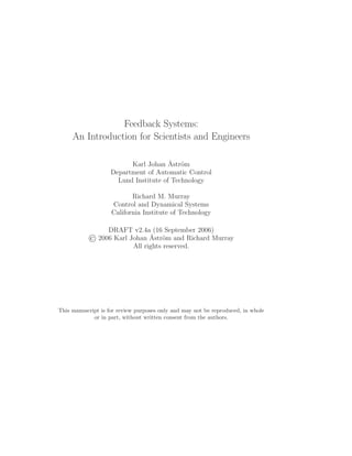
Figure 1.4: Early control devices: (a) Honeywell T86 thermostat, originally intro-
duced in 1953, (b) Chrysler cruise control system, introduced in the 1958 Chrysler
Imperial (note the centrifugal governor) [Row58].
subsystems, a feature that is crucial in the operation of all large engineered
systems.
Control is also closely associated with computer science, since virtu-
ally all modern control algorithms for engineering systems are implemented
in software. However, control algorithms and software are very different
from traditional computer software. The physics (dynamics) of the system
are paramount in analyzing and designing them and their real-time nature
dominates issues of their implementation.
1.3 Feedback Examples
Feedback has many interesting and useful properties. It makes it possible
to design precise systems from imprecise components and to make physical
variables in a system change in a prescribed fashion. An unstable system
can be stabilized using feedback and the effects of external disturbances can
be reduced. Feedback also offers new degrees of freedom to a designer by
exploiting sensing, actuation and computation. In this section we survey
some of the important applications and trends for feedback in the world
around us.

19. 1.3. FEEDBACK EXAMPLES 7
Early Technological Examples
The proliferation of control in engineered systems has occurred primarily
in the latter half of the 20th century. There are some familiar exceptions,
such as the centrifugal governor described earlier and the thermostat (Fig-
ure 1.4a), designed at the turn of the century to regulate temperature of
buildings.
The thermostat, in particular, is often cited as a simple example of feed-
back control that everyone can understand. Namely, the device measures
the temperature in a building, compares that temperature to a desired set
point, and uses the “feedback error” between these two to operate the heat-
ing plant, e.g. to turn heating on when the temperature is too low and to
turn if off when the temperature is too high. This explanation captures the
essence of feedback, but it is a bit too simple even for a basic device such as
the thermostat. Actually, because lags and delays exist in the heating plant
and sensor, a good thermostat does a bit of anticipation, turning the heater
off before the error actually changes sign. This avoids excessive temperature
swings and cycling of the heating plant.
This modification illustrates that, even in simple cases, good control
system design is not entirely trivial. It must take into account the dynamic
behavior of the object being controlled in order to do a good job. The more
complex the dynamic behavior, the more elaborate the modifications. In
fact, the development of a thorough theoretical understanding of the re-
lationship between dynamic behavior and good controllers constitutes the
most significant intellectual accomplishment of the control community, and
the codification of this understanding into powerful computer aided engi-
neering design tools makes all modern control systems possible.
There are many other control system examples that have developed over
the years with progressively increasing levels of sophistication and impact.
An early system with broad public exposure was the “cruise control” option
introduced on automobiles in 1958 (see Figure 1.4b). With cruise control,
ordinary people experienced the dynamic behavior of closed loop feedback
systems in action—the slowdown error as the system climbs a grade, the
gradual reduction of that error due to integral action in the controller, the
small (but unavoidable) overshoot at the top of the climb, etc. More im-
portantly, by experiencing these systems operating reliably and robustly,
the public learned to trust and accept feedback systems, permitting their
increasing proliferation all around us. Later control systems on automobiles
have had more concrete impact, such as emission controls and fuel metering
systems that have achieved major reductions of pollutants and increases in

20. 8 CHAPTER 1. INTRODUCTION
Figure 1.5: The F-18 aircraft, one of the first production military fighters to use “fly-
by-wire” technology, and the X-45 (UCAV) unmanned aerial vehicle. Photographs
courtesy of NASA Dryden Flight Research Center.
fuel economy.
In the industrial world, control systems have been a key enabling tech-
nology for everything from factory automation (starting with numerically
controlled machine tools), to process control in oil refineries and chemical
plants, to integrated circuit manufacturing, to power generation and distri-
bution. Early use of regulators for manufacturing systems has evolved to
the use of hundreds or even thousands of computer controlled subsystems
in major industrial plants.
Aerospace and Transportation
Aerospace and transportation systems encompass a collection of critically
important application areas where control is a central technology. These
application areas represent a significant part of the modern world’s overall
technological capability. They are also a major part of its economic strength,
and they contribute greatly to the well being of its people.
In aerospace, control has been a key technological capability tracing back
to the very beginning of the 20th century. Indeed, the Wright brothers are
correctly famous not simply for demonstrating powered flight but controlled
powered flight. Their early Wright Flyer incorporated moving control sur-
faces (vertical fins and canards) and warpable wings that allowed the pilot to
regulate the aircraft’s flight. In fact, the aircraft itself was not stable, so con-
tinuous pilot corrections were mandatory. This early example of controlled
flight is followed by a fascinating success story of continuous improvements
in flight control technology, culminating in the very high performance, highly

21. 1.3. FEEDBACK EXAMPLES 9
reliable automatic flight control systems we see on modern commercial and
military aircraft today.
Similar success stories for control technology occurred in many other
application areas. Early World War II bombsights and fire control servo
systems have evolved into today’s highly accurate radar-guided guns and
precision-guided weapons. Early failure-prone space missions have evolved
into routine launch operations, manned landings on the moon, permanently
manned space stations, robotic vehicles roving Mars, orbiting vehicles at the
outer planets, and a host of commercial and military satellites serving var-
ious surveillance, communication, navigation, and earth observation needs.
Cars have advanced from manually tuned mechanical/pneumatic technol-
ogy to computer-controlled operation of all major functions, including fuel
injection, emission control, cruise control, braking, and cabin comfort.
Current research in aerospace and transportation systems is investigat-
ing the application of feedback to higher levels of decision making, including
logical regulation of operating modes, vehicle configurations, payload con-
figurations, and health status. These have historically been performed by
human operators, but today that boundary is moving, and control systems
are increasingly taking on these functions. Another dramatic trend on the
horizon is the use of large collections of distributed entities with local com-
putation, global communication connections, very little regularity imposed
by the laws of physics, and no possibility of imposing centralized control
actions. Examples of this trend include the national airspace management
problem, automated highway and traffic management, and the command
and control for future battlefields.
Information and Networks
The rapid growth of communication networks provides several major op-
portunities and challenges for control. Although there is overlap, we can
divide these roughly into two main areas: control of networks and control
over networks.
Control of networks is a large area, spanning many topics, including
congestion control, routing, data caching, and power management. Sev-
eral features of these control problems make them very challenging. The
dominant feature is the extremely large scale of the system; the Internet is
probably the largest feedback control system man has ever built. Another
is the decentralized nature of the control problem: local decisions must be
made quickly and based only on local information. Stability is complicated
by the presence of varying time lags, as information about the network state

22. 10 CHAPTER 1. INTRODUCTION
Figure 1.6: UUNET network backbone for North America. Figure courtesy of
WorldCom.
can only be observed or relayed to controllers after a delay, and the effect of a
local control action can be felt throughout the network only after substantial
delay. Uncertainty and variation in the network, through network topology,
transmission channel characteristics, traffic demand, available resources, and
the like, may change constantly and unpredictably. Other complicating is-
sues are the diverse traffic characteristics—in terms of arrival statistics at
both the packet and flow time scales—and the different requirements for
quality of service that the network must support.
Resources that must be managed in this environment include computing,
storage and transmission capacities at end hosts and routers. Performance of
such systems is judged in many ways: throughput, delay, loss rates, fairness,
reliability, as well as the speed and quality with which the network adapts
to changing traffic patterns, changing resource availability, and changing
network congestion. The robustness and performance of the global Internet
is a testament to the use of feedback to meet the needs of society in the face
of these many uncertainties.
While the advances in information technology to date have led to a global
Internet that allows users to exchange information, it is clear that the next
phase will involve much more interaction with the physical environment and
the increased use of control over networks. Networks of sensor and actua-
tor nodes with computational capabilities, connected wirelessly or by wires,

23. 1.3. FEEDBACK EXAMPLES 11
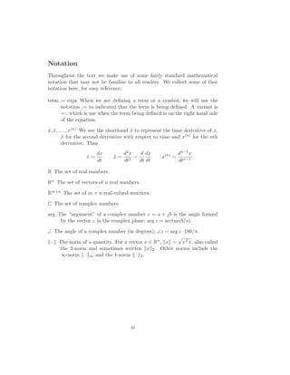
Figure 1.7: “Spirit”, one of the two Mars Exploratory Rovers, and Sony AIBO
Entertainment Robot. Photographs courtesy of Jet Propulsion Laboratory and
Sony.
can form an orchestra that controls our physical environment. Examples
include automobiles, smart homes, large manufacturing systems, intelligent
highways and networked city services, and enterprise-wide supply and logis-
tics chains.
Robotics and Intelligent Machines
Whereas early robots were primarily used for manufacturing, modern robots
include wheeled and legged machines capable of competing in robotic com-
petitions and exploring planets, unmanned aerial vehicles for surveillance
and combat, and medical devices that provide new capabilities to doctors.
Future applications will involve both increased autonomy and increased in-
teraction with humans and with society. Control is a central element in all
of these applications and will be even more important as the next generation
of intelligent machines are developed.
The goal of cybernetic engineering, already articulated in the 1940s and
even before, has been to implement systems capable of exhibiting highly
flexible or “intelligent” responses to changing circumstances. In 1948, the
MIT mathematician Norbert Wiener gave a widely read account of cybernet-
ics [Wie48]. A more mathematical treatment of the elements of engineering
cybernetics was presented by H.S. Tsien in 1954, driven by problems related
to control of missiles [Tsi54]. Together, these works and others of that time
form much of the intellectual basis for modern work in robotics and control.
Two accomplishments that demonstrate the successes of the field are
the Mars Exploratory Rovers and entertainment robots such as the Sony
AIBO, shown in Fig. 1.7. The two Mars Exploratory Rovers, launched by
the Jet Propulsion Laboratory (JPL), maneuvered on the surface of Mars

24. 12 CHAPTER 1. INTRODUCTION
for over two years starting in January 2004 and sent back pictures and
measurements of their environment. The Sony AIBO robot debuted in June
of 1999 and was the first “entertainment” robot to be mass marketed by
a major international corporation. It was particularly noteworthy because
of its use of AI technologies that allowed it to act in response to external
stimulation and its own judgment. This “higher level” of feedback is key
element of robotics, where issues such as task-based control and learning are
prevalent.
Despite the enormous progress in robotics over the last half century, the
field is very much in its infancy. Today’s robots still exhibit extremely simple
behaviors compared with humans, and their ability to locomote, interpret
complex sensory inputs, perform higher level reasoning, and cooperate to-
gether in teams is limited. Indeed, much of Wiener’s vision for robotics and
intelligent machines remains unrealized. While advances are needed in many
fields to achieve this vision—including advances in sensing, actuation, and
energy storage—the opportunity to combine the advances of the AI commu-
nity in planning, adaptation, and learning with the techniques in the control
community for modeling, analysis, and design of feedback systems presents
a renewed path for progress.
Materials and Processing
The chemical industry is responsible for the remarkable progress in develop-
ing new materials that are key to our modern society. Process manufacturing
operations require a continual infusion of advanced information and process
control technologies in order for the chemical industry to maintain its global
ability to deliver products that best serve the customer reliably and at the
lowest cost. In addition, several new technology areas are being explored
that will require new approaches to control to be successful. These range
from nanotechnology in areas such as electronics, chemistry, and biomateri-
als to thin film processing and design of integrated microsystems to supply
chain management and enterprise resource allocation. The payoffs for new
advances in these areas are substantial, and the use of control is critical to
future progress in sectors from semiconductors to pharmaceuticals to bulk
materials.
There are several common features within materials and processing that
pervade many of the applications. Modeling plays a crucial role, and there is
a clear need for better solution methods for multidisciplinary systems com-
bining chemistry, fluid mechanics, thermal sciences, and other disciplines
at a variety of temporal and spatial scales. Better numerical methods for

25. 1.3. FEEDBACK EXAMPLES 13
Figure 1.8: Intel Pentium IV wafer and die. Photographs courtesy of Intel.
traversing these scales and designing, controlling, and optimizing under un-
certainty are also needed. And control techniques must make use of increased
in situ measurements to control increasingly complex phenomena.
In addition to the continuing need to improve product quality, several
other factors in the process control industry are drivers for the use of control.
Environmental statutes continue to place stricter limitations on the produc-
tion of pollutants, forcing the use of sophisticated pollution control devices.
Environmental safety considerations have led to the design of smaller storage
capacities to diminish the risk of major chemical leakage, requiring tighter
control on upstream processes and, in some cases, supply chains. And large
increases in energy costs have encouraged engineers to design plants that are
highly integrated, coupling many processes that used to operate indepen-
dently. All of these trends increase the complexity of these processes and
the performance requirements for the control systems, making the control
system design increasingly challenging.
As in many other application areas, new sensor technology is creating
new opportunities for control. Online sensors—including laser backscatter-
ing, video microscopy, ultraviolet, infrared, and Raman spectroscopy—are
becoming more robust and less expensive and are appearing in more manu-
facturing processes. Many of these sensors are already being used by current
process control systems, but more sophisticated signal processing and con-
trol techniques are needed to more effectively use the real-time information
provided by these sensors. Control engineers can also contribute to the
design of even better sensors, which are still needed, for example, in the
microelectronics industry. As elsewhere, the challenge is making use of the

26. 14 CHAPTER 1. INTRODUCTION
large amounts of data provided by these new sensors in an effective manner.
In addition, a control-oriented approach to modeling the essential physics
of the underlying processes is required to understand fundamental limits on
observability of the internal state through sensor data.
Instrumentation
Feedback has had a major impact on instrumentation. Consider for example
an accelerometer, where early instruments consisted of a mass suspended on
a spring with a deflection sensor. The precision of such an instrument de-
pends critically on accurate calibration of spring and the sensor. There is
also a design compromise because a weak spring gives high sensitivity but
also low bandwidth. An accelerometer based on feedback uses instead a
voice coil to keep the mass at a given position and the acceleration is pro-
portional to the current through the voice coil. In such an instrument the
precision depends entirely on the calibration of the voice coil and does not
depend on the sensor, which is only used as the feedback signal. The sen-
sitivity bandwidth compromise is also avoided. This way of using feedback
was applied to practically all engineering fields and it resulted in instruments
with drastically improved performance. The development of inertial naviga-
tion where position is determined from gyroscopes and accelerometers which
permits accurate guidance and control of vehicles is a spectacular example.
There are many other interesting and useful applications of feedback in
scientific instruments. The development of the mass spectrometer is an early
example. In a paper from 1935 by Nier it is observed that the deflection
of the ions depend on both the magnetic and the electric fields. Instead of
keeping both fields constant, Nier let the magnetic field fluctuate and the
electric field was controlled to keep the ratio of the fields constant. The
feedback was implemented using vacuum tube amplifiers. The scheme was
crucial for the development of mass spectroscopy.
Another example is the work by the Dutch Engineer van der Meer. He
invented a clever way to use feedback to maintain a high density and good
quality of the beam of a particle accelerator. The idea is to sense particle
displacement at one point in the accelerator and apply a correcting signal
at another point. The scheme, called stochastic cooling, was awarded the
Nobel Prize in Physics in 1984. The method was essential for the successful
experiments in CERN when the existence of the particles W and Z was first
demonstrated.
The 1986 Nobel Prize in Physics—awarded to Binnig and Rohrer for
their design of the scanning tunneling microscope—is another example of

27. 1.3. FEEDBACK EXAMPLES 15
clever use of feedback. The key idea is to move a narrow tip on a cantilever
beam across the surface and to register the forces on the tip. The deflection
of the tip was measured using tunneling which gave an extreme accuracy so
that individual atoms could be registered.
A severe problem in astronomy is that turbulence in the atmosphere
blurs images in telescopes because of variations in diffraction of light in the
atmosphere. The blur is of the order of an arc-second in a good telescope.
One way to eliminate the blur is to move the telescope outside the Earths
atmosphere as is done with the Hubble telescope. Another way is to use
feedback to eliminate the effects of the variations in a telescope on the Earth
which is the idea of “adaptive optics.” The reference signal is a bright star
or an artificial laser beam projected into the atmosphere. The actuator is a
deformable mirror which can have hundreds or thousands of elements. The
error signal is formed by analyzing the shape of the distorted wave form
from the reference. This signal is sent to the controller which adjusts the
deformable mirror. The light from the observed star is compensated because
it is also reflected in the deformable mirror before it is sent to the detector.
The wave lengths used for observation and control are often different. Since
diffraction in the atmosphere changes quite rapidly the response time of the
control system must be of the order of milliseconds.
Feedback in Nature
Many cutting edge problems in the natural sciences involve understanding
aggregate behavior in complex large-scale systems. This behavior “emerges”
from the interaction of a multitude of simpler systems, with intricate pat-
terns of information flow. Representative examples can be found in fields
ranging from embryology to seismology. Researchers who specialize in the
study of specific complex systems often develop an intuitive emphasis on
analyzing the role of feedback (or interconnection) in facilitating and sta-
bilizing aggregate behavior, and it is often noted that one can only have
hope of deep understanding if it is somehow possible for theories of collec-
tive phenomenology to be robust to inevitable uncertainties in the modeling
of fine-scale dynamics and interconnection.
While sophisticated theories have been developed by domain experts
for the analysis of various complex systems, the development of rigorous
methodology that can discover and exploit common features and essential
mathematical structure is just beginning to emerge. Advances in science and
technology are creating new understanding of the underlying dynamics and
the importance of feedback in a wide variety of natural and technological

28. 16 CHAPTER 1. INTRODUCTION
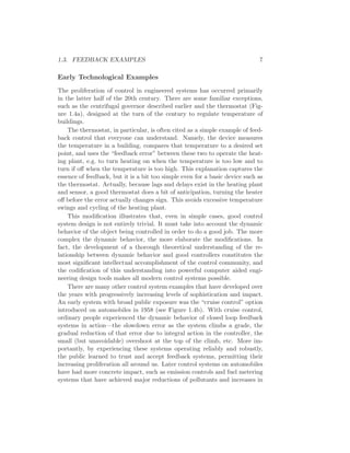
Figure 1.9: The wiring diagram of the growth signaling circuitry of the mammalian
cell [HW00].
systems We briefly highlight four application areas here.
Biological Systems. At a variety of levels of organization—from molec-
ular to cellular to organismal to populational—biology is becoming more
accessible to approaches that are commonly used in engineering: mathe-
matical modeling, systems theory, computation, and abstract approaches to
synthesis. Conversely, the accelerating pace of discovery in biological science
is suggesting new design principles that may have important practical appli-
cations in man-made systems. This synergy at the interface of biology and
engineering offers unprecedented opportunities to meet challenges in both
areas. The principles of feedback and control are central to many of the
key questions in biological engineering and will play an enabling role in the
future of this field.
A major theme currently underway in the biology community is the
science of reverse (and eventually forward) engineering of biological control
networks (such as the one shown in Figure 1.9). There are a wide variety
of biological phenomena that provide a rich source of examples for control,
including gene regulation and signal transduction; hormonal, immunological,
and cardiovascular feedback mechanisms; muscular control and locomotion;
active sensing, vision, and proprioception; attention and consciousness; and

29. 1.3. FEEDBACK EXAMPLES 17
population dynamics and epidemics. Each of these (and many more) provide
opportunities to figure out what works, how it works, and what we can do
to affect it.
Ecosystems. In contrast to individual cells and organisms, emergent
properties of aggregations and ecosystems inherently reflect selection mech-
anisms which act on multiple levels, and primarily on scales well below that
of the system as a whole. Because ecosystems are complex, multiscale dy-
namical systems, they provide a broad range of new challenges for modeling
and analysis of feedback systems. Recent experience in applying tools from
control and dynamical systems to bacterial networks suggests that much of
the complexity of these networks is due to the presence of multiple layers of
feedback loops that provide robust functionality to the individual cell. Yet
in other instances, events at the cell level benefit the colony at the expense
of the individual. Systems level analysis can be applied to ecosystems with
the goal of understanding the robustness of such systems and the extent
to which decisions and events affecting individual species contribute to the
robustness and/or fragility of the ecosystem as a whole.
Quantum Systems. While organisms and ecosystems have little to do
with quantum mechanics in any traditional scientific sense, complexity and
robustness issues very similar to those described above can be identified in
the modern study of quantum systems. In large part, this sympathy arises
from a trend towards wanting to control quantum dynamics and to harness
it for the creation of new technological devices. At the same time, physicists
are progressing from the study of elementary quantum systems to the study
of large aggregates of quantum components, and it has been recognized that
dynamical complexity in quantum systems increases exponentially faster
with system size than it does in systems describable by classical (macro-
scopic) physics. Factors such as these are prompting the physics community
to search broadly for new tools for understanding robust interconnection
and emergent phenomena.
Modern scientific research is rapidly evolving a field of quantum engi-
neering. Driven by technology goals in areas such as quantum informa-
tion processing, nano-electromechanical sensing, chemical synthesis, trace
gas detection, and ultrahigh-bandwidth optical communication, researchers
are beginning to formulate strategies for achieving robust performance with
physical devices or systems in which quantum mechanical effects are promi-
nent. Mathematical tools from control and dynamical systems for analysis
and synthesis could have a profound impact on activities of this kind. A
schematic diagram of a modern quantum control experiment is show in Fig-
ure 1.10a.

30. 18 CHAPTER 1. INTRODUCTION
(a) (b)
Figure 1.10: Examples of feedback systems in nature: (a) quantum control system
and (b) global carbon cycle.
Environmental Science. It is now indisputable that human activities
have altered the environment on a global scale. Problems of enormous
complexity challenge researchers in this area and first among these is to
understand the feedback systems that operate on the global scale. One of
the challenges in developing such an understanding is the multiscale nature
of the problem, with detailed understanding of the dynamics of microscale
phenomena such as microbiological organisms being a necessary component
of understanding global phenomena, such as the carbon cycle illustrated
Figure 1.10b.
Other Areas
The previous sections have described some of the major application areas
for control. However, there are many more areas where ideas from control
are being applied or could be applied. Some of these include: economics
and finance, including problems such as pricing and hedging options; energy
systems, including load distribution and power management for the elec-
trical grid; and manufacturing systems, including supply chains, resource
management and scheduling, and factory automation.

31. 1.4. FEEDBACK PROPERTIES 19
Compute
Actuate
Throttle
Sense
Speed
0 5 10 15
20
25
30
35
time (sec)
speed(m/s)
m = 1000 kg
m = 2000 kg
m = 3000 kg
Figure 1.11: A simple feedback system for controlling the speed of a vehicle.
1.4 Feedback Properties
Feedback is a powerful idea which, as we have seen, is used extensively in
natural and technological systems. The principle of feedback is very simple:
base correcting actions on the difference between desired and actual perfor-
mance. In engineering, feedback has been rediscovered and patented many
times in many different contexts. The use of feedback has often resulted in
vast improvements in system capability and these improvements have some-
times been revolutionary, as discussed above. The reason for this is that
feedback has some truly remarkable properties. In this section we will dis-
cuss some of the properties of feedback that can be understood intuitively.
This intuition will be formalized in the subsequent chapters.
Robustness to Uncertainty
One of the key uses of feedback is to provide robustness to uncertainty. By
measuring the difference between the sensed value of a regulated signal and
its desired value, we can supply a corrective action. If the system undergoes
some change that affects the regulated signal, then we sense this change and
try to force the system back to the desired operating point. This is precisely
the effect that Watt exploited in his use of the centrifugal governor on steam
engines.
As an example of this principle, consider the simple feedback system
shown in Figure 1.11a. In this system, the speed of a vehicle is controlled by
adjusting the amount of gas flowing to the engine. A simple “proportional
plus integral” feedback is used to to make the amount of gas depend on
both the error between the current and desired speed, and the integral of
that error. The plot on the right shows the results of this feedback for a
step change in the desired speed and a variety of different masses for the car

32. 20 CHAPTER 1. INTRODUCTION
(which might result from having a different number of passengers or towing
a trailer). Notice that independent of the mass (which varies by a factor
of 3), the steady state speed of the vehicle always approaches the desired
speed and achieves that speed within approximately 5 seconds. Thus the
performance of the system is robust with respect to this uncertainty.
Another early example of the use of feedback to provide robustness was
the negative feedback amplifier. When telephone communications were de-
veloped, amplifiers were used to compensate for signal attenuation in long
lines. The vacuum tube was a component that could be used to build ampli-
fiers. Distortion caused by the nonlinear characteristics of the tube amplifier
together with amplifier drift were obstacles that prevented development of
line amplifiers for a long time. A major breakthrough was invention of the
feedback amplifier in 1927 by Harold S. Black, an electrical engineer at the
Bell Telephone Laboratories. Black used negative feedback which reduces
the gain but makes the amplifier very insensitive to variations in tube char-
acteristics. This invention made it possible to build stable amplifiers with
linear characteristics despite nonlinearities of the vacuum tube amplifier.
Design of Dynamics
Another use of feedback is to change the dynamics of a system. Through
feedback, we can alter the behavior of a system to meet the needs of an
application: systems that are unstable can be stabilized, systems that are
sluggish can be made responsive, and systems that have drifting operating
points can be held constant. Control theory provides a rich collection of
techniques to analyze the stability and dynamic response of complex systems
and to place bounds on the behavior of such systems by analyzing the gains
of linear and nonlinear operators that describe their components.
An example of the use of control in the design of dynamics comes from
the area of flight control. The following quote, from a lecture by Wilbur
Wright to the Western Society of Engineers in 1901 [McF53], illustrates the
role of control in the development of the airplane:
“Men already know how to construct wings or airplanes, which
when driven through the air at sufficient speed, will not only
sustain the weight of the wings themselves, but also that of the
engine, and of the engineer as well. Men also know how to build
engines and screws of sufficient lightness and power to drive these
planes at sustaining speed ... Inability to balance and steer still
confronts students of the flying problem. ... When this one

33. 1.4. FEEDBACK PROPERTIES 21
Figure 1.12: The Curtiss-Sperry E in 1912 (left) and a closeup of the Sperry Au-
topilot (right).
feature has been worked out, the age of flying will have arrived,
for all other difficulties are of minor importance.”
The Wright brothers thus realized that control was a key issue to enable
flight. They resolved the compromise between stability and maneuverability
by building an airplane, Kitty Hawk, that was unstable but maneuverable.
Kitty Hawk had a rudder in the front of the airplane, which made the plane
very maneuverable. A disadvantage was the necessity for the pilot to keep
adjusting the rudder to fly the plane: if the pilot let go of the stick the plane
would crash. Other early aviators tried to build stable airplanes. These
would have been easier to fly, but because of their poor maneuverability
they could not be brought up into the air. By using their insight and skillful
experiments the Wright brothers made the first successful flight with Kitty
Hawk in 1905.
Since it was quite tiresome to fly an unstable aircraft, there was strong
motivation to find a mechanism that would stabilize an aircraft. Such a
device, invented by Sperry, was based on the concept of feedback. Sperry
used a gyro-stabilized pendulum to provide an indication of the vertical. He
then arranged a feedback mechanism that would pull the stick to make the
plane go up if it was pointing down and vice versa. The Sperry autopilot is
the first use of feedback in aeronautical engineering and Sperry won a prize
in a competition for the safest airplane in Paris in 1912. Figure 1.12 shows
the Curtiss-Sperry seaplane and the Sperry autopilot. The autopilot is a
good example of how feedback can be used to stabilize an unstable system
and hence “design the dynamics” of the aircraft.
One of the other advantages of designing the dynamics of a device is
that it allows for increased modularity in the overall system design. By us-

34. 22 CHAPTER 1. INTRODUCTION
Supervisory Control
Actuation
Vehicle
Follower
Path
State
Estimator
Planner
Path
Sensors
Terrain
Map
Elevation
Map
Cost
Finding
Road
Vehicle
Figure 1.13: DARPA Grand Challenge: (a) “Alice,” Team Caltech’s entry in the
2005 competition. (b) Networked control architecture used by Alice.
ing feedback to create a system whose response matches a desired profile, we
can hide the complexity and variability that may be present inside a subsys-
tem. This allows creation us to create more complex systems by not having
to simultaneously tune the response of a large number of interacting com-
ponents. This was one of the advantages of Black’s use of negative feedback
in vacuum tube amplifiers: the resulting device had a well-defined linear
input/output response that did not depend on the individual characteristics
of the vacuum tubes begin used.
Higher Levels of Automation
A major trend in the use of feedback is its use in higher levels of automation
and decision making. A good example of this is the DARPA Grand Chal-
lenge, a competition sponsored by the US government to build a vehicle that
could autonomously drive itself across the desert. Caltech competed in the
2005 Grand Challenge using a modified Ford E-350 offroad van, nicknamed
“Alice.” It was fully automated, including electronically controlled steering,
throttle, brakes, transmission, and ignition. Its sensing systems included 4
black and white cameras sampling at 30 Hz (arranged in two stereo pairs),
1 color camera for finding roads, 5 LADAR (laser radar) units scanning
at 10 Hz, and a GPS/IMU package capable of providing full position and
orientation at 2.5 millisecond temporal resolution. Computational resources
included 7 high speed servers connected together through a 1 Gb/s Ethernet
switch. A picture of the vehicle is shown in Figure 1.13a.
Custom software was used to control the vehicle. The control system
architecture is shown in Figure 1.13b. This information-rich feedback system
fused data from multiple cameras and LADAR units to determine a digital
elevation map for the terrain around it and then used this map to compute

35. 1.4. FEEDBACK PROPERTIES 23
a speed map that estimated the speed at which the vehicle could drive in
the environment. The map was modified to include additional information
where roads were identified (through vision-based algorithms) and where no
data was present (due to hills or temporary sensor outages). This speed map
was then used by an optimization-based planner to determine the path that
would allow the vehicle to make the most progress in a fixed period of time.
The commands from the planner were sent to a trajectory tracking algorithm
that compared the desired vehicle position to its estimated position (from
GPS/IMU data) and issued appropriate commands to the steering, throttle
and brake actuators. Finally, a supervisor control module performed higher
level tasks, including implementing strategies for making continued forward
progress if one of the hardware or software components failed temporarily
(either due to external or internal conditions).
The software and hardware infrastructure that was developed enabled
the vehicle to traverse long distances at substantial speeds. In testing, Alice
drove itself over 500 kilometers in the Mojave Desert of California, with the
ability to follow dirt roads and trails (if present) and avoid obstacles along
the path. Speeds of over 50 km/hr were obtained in fully autonomous mode.
Substantial tuning of the algorithms was done during desert testing, in part
due to the lack of systems-level design tools for systems of this level of com-
plexity. Other competitors in the race (including Stanford, which one the
competition) used algorithms for adaptive control and learning, increasing
the capabilities of their systems in unknown environments. Together, the
competitors in the grand challenge demonstrated some of the capabilities
for the next generation of control systems and highlighted many research
directions in control at higher levels of decision making.
Drawbacks of Feedback
While feedback has many advantages, it also has some drawbacks. Chief
among these is the possibility for instability if the system is not designed
properly. We are all familiar with the effects of “positive feedback” when
the amplification on a microphone is turned up too high in a room. This is
an example of a feedback instability, something that we obviously want to
avoid. This is tricky because of the uncertainty that feedback was introduced
to compensate for: not only must we design the system to be stable with
the nominal system we are designing for, but it must remain stable under
all possible perturbations of the dynamics.
In addition to the potential for instability, feedback inherently couples
different parts of a system. One common problem that feedback inherently

36. 24 CHAPTER 1. INTRODUCTION
injects measurement noise into the system. In engineering systems, measure-
ments must be carefully filtered so that the actuation and process dynamics
do not respond to it, while at the same time insuring that the measurement
signal from the sensor is properly coupled into the closed loop dynamics (so
that the proper levels of performance are achieved).
Another potential drawback of control is the complexity of embedding
a control system into a product. While the cost of sensing, computation,
and (to a lesser extent) actuation has decreased dramatically in the past
few decades, the fact remains that control systems are often very compli-
cated and hence one must carefully balance the costs and benefits. An early
engineering example of this is the use of microprocessor-based feedback sys-
tems in automobiles. The use of microprocessors in automotive applications
began in the early 1970s and was driven by increasingly strict emissions
standards, which could only be met through electronic controls. Early sys-
tems were expensive and failed more often than desired, leading to frequent
customer dissatisfaction. It was only through aggressive improvements in
technology that the performance, reliability and cost of these systems al-
lowed them to be used in a transparent fashion. Even today, the complexity
of these systems is such that it is difficult for an individual car owner to
fix problems. There have also been spectacular failures due to unexpected
interactions.
Feedforward
When using feedback that there must be an error before corrective actions
are taken. Feedback is thus reactive. In some circumstances it is possible to
measure a disturbance before it enters the system and this information can
be used to take corrective action before the disturbance has influenced the
system. The effect of the disturbance is thus reduced by measuring it and
generating a control signal that counteracts it. This way of controlling a
system is called feedforward. Feedforward is particularly useful to shape the
response to command signals because command signals are always available.
Since feedforward attempts to match two signals, it requires good process
models otherwise the corrections may have the wrong size or it may be badly
timed.
The ideas of feedback and feedforward are very general and appear in
many different fields. In economics, feedback and feedforward are analogous
to a market-based economy versus a planned economy. In business a pure
feedforward strategy corresponds to running a company based on extensive
strategic planning while a feedback strategy corresponds to a pure reactive

37. 1.5. SIMPLE FORMS OF FEEDBACK 25
approach. The experience in control indicates that it is often advantageous
to combine feedback and feedforward. Feedforward is particularly useful
when disturbances can be measured or predicted. A typical example is in
chemical process control where disturbances in one process may be due to
processes upstream. The correct balance of the approaches requires insight
and understanding of their properties.
Positive Feedback
In most of this text, we will consider the role of negative feedback, in which
we attempt to regulate the system by reacting to disturbances in a way that
decreases the effect of those disturbances. In some systems, particularly
biological systems, positive feedback can play an important role. In a system
with positive feedback, the increase in some variable or signal leads to a
situation in which that quantify is further through its dynamics. This has
a destabilizing effect and is usually accompanied by a saturation that limits
the growth of the quantity. Although often considered undesirable, this
behavior is used in biological (and engineering) systems to obtain a very
fast response to a condition or signal.
1.5 Simple Forms of Feedback
The idea of feedback to make corrective actions based on the difference be-
tween the desired and the actual value can be implemented in many different
ways. The benefits of feedback can be obtained by very simple feedback laws
such as on-off control, proportional control and PID control. In this section
we provide a brief preview of some of the topics that will be studied more
formally in the remainder of the text.
A simple feedback mechanism can be described as follows:
u =
umax if e > 0
umin if e < 0
(1.1)
where e = r−y is the difference between the reference signal and the output
of the system. Figure 1.14a shows the relation between error and control.
This control law implies that maximum corrective action is always used.
The feedback in equation (1.1) is called on-off control. One of its chief
advantages is that it is simple and there are no parameters to choose. On-off
control often succeeds in keeping the process variable close to the reference,
such as the use of a simple thermostat to maintain the temperature of a

38. 26 CHAPTER 1. INTRODUCTION
(c)
e
u
e
u
e
u
(a) (b)
Figure 1.14: Controller characteristics for ideal on-off control (a), and modifications
with dead zone (b) and hysteresis (c).
room. It typically results in a system where the controlled variables oscillate,
which is often acceptable if the oscillation is sufficiently small.
Notice that in equation (1.1) the control variable is not defined when the
error is zero. It is common to have some modifications either by introducing
hysteresis or a dead zone (see Figure 1.14b and 1.14c).
The reason why on-off control often gives rise to oscillations is that the
system over reacts since a small change in the error will make the actuated
variable change over the full range. This effect is avoided in proportional
control, where the characteristic of the controller is proportional to the con-
trol error for small errors. This can be achieved by making the control signal
proportional to the error, which gives the control law
u =



umax if e > emax
ke if emin ≤ e ≤ emax
umin if e < emin,
(1.2)
where where k is the controller gain, emin = umin/k, and emax = umax/k.
The interval (emin, emax) is called the proportional band because the behavior
of the controller is linear when the error is in this interval:
u = k(r − y) = ke if emin ≤ e ≤ emax. (1.3)
While a vast improvement over on-off control, proportional control has
the drawback that the process variable often deviates from its reference
value. In particular, if some level of control signal is required for the system
to maintain a desired value, then we must have e = 0 in order to generate
the requisite input.
This can be avoided by making the control action proportional to the

39. 1.5. SIMPLE FORMS OF FEEDBACK 27
integral of the error:
u(t) = ki
t
0
e(τ)dτ. (1.4)
This control form is called integral control and ki is the integral gain. It can
be shown through simple arguments that a controller with integral action
will have zero “steady state” error (Exercise 5). The catch is that there may
not always be a steady state because the system may be oscillating. This
property has been rediscovered many times and is one of the properties that
have strongly contributed to the wide applicability of integral controllers.
An additional refinement is to provide the controller with an anticipative
ability by using a prediction of the error. A simple prediction is given by
the linear extrapolation
e(t + Td) ≈ e(t) + Td
de(t)
dt
,
which predicts the error Td time units ahead. Combining proportional, in-
tegral and derivative control we obtain a controller that can be expressed
mathematically as follows:
u(t) = ke(t) + ki
t
0
e(τ) dτ + kd
de(t)
dt
= k e(t) +
1
Ti
t
0
e(τ) dτ + Td
de(t)
dt
(1.5)
The control action is thus a sum of three terms: the past as represented
by the integral of the error, the present as represented by the proportional
term, and the future as represented by a linear extrapolation of the error
(the derivative term). This form of feedback is called a PID controller and
its action is illustrated in Figure 1.15.
The PID controller is very useful and is capable of solving a wide range of
control problems. The PI controller, in which the derivative term is omitted,
is one of the most common forms of the controller. It is quoted that about
90% of all control problems can be solved by PID control, although many
of these controllers are actually PI controllers because derivative action is
often not included. There are more advanced controllers which differ from
the PID controller by using more sophisticated methods for prediction.

40. 28 CHAPTER 1. INTRODUCTION
0000000000
00000
1111111111
11111
000111000000111111
Present
FuturePast
t t + Td
Error
Time
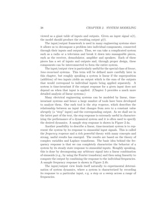
Figure 1.15: A PID controller takes control action based on past, present and future
control errors.
1.6 Control Tools
The development of a control system consists of the tasks modeling, analysis,
simulation, architectural design, design of control algorithms, implementa-
tion, commissioning and operation. Because of the wide use of feedback in
a variety of applications, there has been substantial mathematical develop-
ment in the field of control theory. In many cases the results have also been
packaged in software tools that simplifies the design process. We briefly
describe some of the tools and concepts here.
Modeling
Models play an essential role in analysis and design of feedback systems.
Several sophisticated tools have been developed to build models that are
suited for control.
Models can often be obtained from first principles and there are several
modeling tools in special domains such as electric circuits and multibody sys-
tems. Since control applications cover such a wide range of domains it is also
desirable to have modeling tools that cut across traditional discipline bound-
aries. Such modeling tools are now emerging, with the models obtained by
cutting a system into subsystems and writing equations for balance of mass,
energy and momentum, and constitutive equations that describe material
properties for each subsystem. Object oriented programming can be used
very effectively to organize the work and extensive symbolic computation
can be used to simplify the equations. Models and components can then be
organized in libraries for efficient reuse. Modelica [Til01] is an example of a
modeling tool of this type.

41. 1.6. CONTROL TOOLS 29
Modeling from input/output data or system identification is another ap-
proach to modeling that has been developed in control. Direct measurement
of the response to step input is commonly used in the process industry to
tune proportional-integral (PI) controllers. More accurate models can be
obtained by measuring the response to sinusoidal signals, which is partic-
ularly useful for systems with fast response time. Control theory has also
developed new techniques for modeling dynamics and disturbances, includ-
ing input/output representations of systems (how disturbances propagate
through the system) and data-driven system identification techniques. The
use of “forced response” experiments to build models of systems is well devel-
oped in the control field and these tools find application in many disciplines,
independent of the use of feedback.
Finally, one of the hallmarks of modern control engineering is the devel-
opment of model reduction techniques that allow a hierarchy of models to
be constructed at different levels of fidelity. This was originally motivated
by the need to produce low complexity controllers that could be imple-
mented with limited computation. The theory is well developed for linear
systems and is now used to produce models of varying levels of complexity
with bounds on the input/output errors corresponding to different approx-
imations. Model reduction for general classes of nonlinear systems is an
important unsolved problem.
The impact of modeling on engineering and control over the past 50 years
has been profound. Today, entire products are designed using only models,
with the first prototype being a fully working system. Doing this requires
an enormous amount of infrastructure in simulation tools, detailed physical
models, and experience in using models. Moving forward, this infrastructure
becomes even more important as suppliers of components compete and sell
their products based on detailed models of their systems which implement
the specifications of their products sometimes before the system has even
been built.
Analysis
Control theory has developed an extensive collection of theory and soft-
ware tools for analysis of feedback systems. These tools include stability
analysis for both linear and nonlinear systems, performance measures for
input/output systems, and evaluation of robustness. For robustness analy-
sis, the tools are particularly sophisticated in the case of linear dynamical
systems, where it is possible to analyze the stability and performance of
the system in the presence of external disturbances, parametric uncertainty

42. 30 CHAPTER 1. INTRODUCTION
(e.g., unknown values of parameters such as mass or reaction rates), and un-
modeled dynamics. In the case of unmodeled dynamics, one can even reason
about the performance of a system without knowing the precise behavior of
every subsystem, a very powerful concept.
In almost all cases, the theory used for analysis of feedback systems is
implemented in software tools that can be used in computer aided design en-
vironments. Two very common environments for this analysis are MATLAB
and Mathematica. In both cases, toolboxes are available that implement the
common calculations described in this text (and many more) and these have
become indispensable aides for modern design. More sophisticated tools, ca-
pable of constructing and analyzing very complex hierarchical models, are
also available for more discipline-specific environments.
An important point to remember about systems analysis is that it relies
on models to describe the behavior of the system. In the simplest case,
these models are simulated to provide information about how the system will
respond to a given set of initial conditions, disturbances, and environment.
But modern computational tools can do much more than just simulate the
system, and can provide very sophisticated analyses that answer questions
about the parametric behavior of systems, tradeoffs between different design
factors, and even provide certificates (proofs) of performance. These tools
are very well developed for linear systems, but recent advances in nonlinear
analysis are quickly extending these results to larger and larger classes of
systems.
Synthesis
In addition to tools for analysis of feedback systems, theory and software
has also been developed for synthesizing feedback systems. As an example,
consider the control system depicted in Figure 1.3 on page 5. Given models of
the process to be controlled, it is today possible to automatically synthesize a
control algorithm that satisfies a given performance specification. A typical
approach to doing this would involve first obtaining a nonlinear model for
the process that captured the key behavior that one was interested in. This
model would then be “linearized” around a desired operating point (this is
described in Chapter 5) and a performance condition specified (usually as
a function that one wishes to minimize). Given the linear model and the
control specification, a feedback law can be computed that is the optimal
law for the given specification.
Modern implementation environments continue by allowing this control
algorithm to be “autocoded”, so that programming code implementing the

43. 1.7. FURTHER READING 31
control logic is automatically generated. This has the advantage that the
code generator can be carefully verified so that the resulting algorithm is
correct (as opposed to hand coding the algorithm, which can lead to er-
rors in translation). This autocoded control logic is then downloaded to a
dedicated computing platform with the proper interfaces to the hardware
and implemented. In addition to simple feedback algorithms, most modern
control environments allow complex decision-making logic to be constructed
via block diagrams and this is also automatically compiled and downloaded
to a computer that is connected to the hardware.
This mechanism for generating control algorithms directly from speci-
fications has vastly improved the productivity of control engineers and is
now standard practice in many application areas. It also provides a clear
framework in which new advances, such as real-time, optimization-based
control, can be transitioned to applications quickly and efficiently through
the generation of standard toolboxes.
1.7 Further Reading
The material in this section draws heavily from the report of the Panel
on Future Directions on Control, Dynamics, and Systems [Mur03]. Several
recent papers and reports highlighted successes of control [NS99] and new
vistas in control [Bro00, Kum01]. A fascinating examination of some of
the early history of control in the United States has been written by Min-
dell [Min02]. Additional historical overviews of the field have been prepared
by Bennett [Ben86a, Ben86b] and Mayr[May70], which go back as far as the
1800s. A popular book that describes many control concepts across a wide
range of disciplines is “Out of Control” by Kelly [Kel94].
There are many textbooks available that describe control systems in the
context of specific disciplines. For engineers, the textbooks by Franklin,
Powell and Emami-Naeni [FPEN05], Dorf and Bishop [DB04], Kuo and
Golnaraghi [KG02], and Seborg, Edgar and Mellichamp [SEM03] are widely
used. A number of books look at the role of dynamics and feedback in biolog-
ical systems, including Milhorn [Mil66] (now out of print), Murray [Mur04]
and Ellner and Guckenheimer [EG05]. There is not yet a textbook targeted
specifically at the physics community, although a recent tutorial article by
Bechhoefer [Bec05] covers many specific topics of interest to that community.

44. 32 CHAPTER 1. INTRODUCTION
1.8 Exercises
1. Identify 5 feedback systems that you encounter in your everyday envi-
ronment. For each system, identify the sensing mechanism, actuation
mechanism, and control law. Describe the uncertainty that the feed-
back system provides robustness with respect to and/or the dynamics
that are changed through the use of feedback.
2. Perform the following experiment and explain your results: Holding
your head still, move your right or left hand back and forth in front
of your face, following it with your eyes. Record how quickly you can
move your hand before you begin to lose track of your hand. Now
hold your hand still and move your head back and forth, once again
recording how quickly you can move before loosing track.
3. Balance yourself on one foot with your eyes closed for 15 seconds.
Using Figure 1.3 as a guide, describe the control system responsible
for keeping you from falling down. Note that the “controller” will
differ from the diagram (unless you are an android reading this in the
far future).
4. Download the MATLAB code used to produce Figure 1.11 from the
companion web site. Using trial and error, change the parameters of
the control law so that the overshoot in the speed is not more than 1
m/s for a vehicle with mass m = 1000kg.
5. We say that an system with a constant input reaches “steady state” if
the output of the system approaches a constant value as time increases.
Show that a controller with integral action, such as those given in
equations (1.4) and (1.5), gives zero error if the closed loop system
reaches steady state.

45. Chapter 2
System Modeling
... I asked Fermi whether he was not impressed by the agreement between
our calculated numbers and his measured numbers. He replied, “How many
arbitrary parameters did you use for your calculations?” I thought for a
moment about our cut-off procedures and said, “Four.” He said, “I remember
my friend Johnny von Neumann used to say, with four parameters I can fit
an elephant, and with five I can make him wiggle his trunk.”
Freeman Dyson on describing the predictions of his model for meson-proton
scattering to Enrico Fermi in 1953 [Dys04].
A model is a precise representation of a system’s dynamics used to answer
questions via analysis and simulation. The model we choose depends on the
questions we wish to answer, and so there may be multiple models for a single
physical system, with different levels of fidelity depending on the phenomena
of interest. In this chapter we provide an introduction to the concept of
modeling, and provide some basic material on two specific methods that are
commonly used in feedback and control systems: differential equations and
difference equations.
2.1 Modeling Concepts
A model is a mathematical representation of a physical, biological or in-
formation system. Models allow us to reason about a system and make
predictions about how a system will behave. In this text, we will mainly
be interested in models of dynamical systems describing the input/output
behavior of systems and often in so-called “state space” form.
Roughly speaking, a dynamical system is one in which the effects of
actions do not occur immediately. For example, the velocity of a car does not
33

46. 34 CHAPTER 2. SYSTEM MODELING
change immediately when the gas pedal is pushed nor does the temperature
in a room rise instantaneously when a heater is switched on. Similarly,
a headache does not vanish right after an aspirin is taken, requiring time
to take effect. In business systems, increased funding for a development
project does not increase revenues in the short term, although it may do so
in the long term (if it was a good investment). All of these are examples of
dynamical systems, in which the behavior of the system evolves with time.
Dynamical systems can be viewed in two different ways: the internal
view or the external view. The internal view attempts to describe the in-
ternal workings of the system and originates from classical mechanics. The
prototype problem was describing the motion of the planets. For this prob-
lem it was natural to give a complete characterization of the motion of all
planets. This involves careful analysis of the effects of gravitational pull and
the relative positions of the planets in a system. A major tool in the internal
view is differential equations.
The other view on dynamics originated in electrical engineering. The
prototype problem was to describe electronic amplifiers, where it was natural
to view an amplifier as a device that transforms input voltages to output
voltages and disregard the internal details of the amplifier. This resulted in
the input/output, or external, view of systems. For this type of model, much
more emphasis is placed on how a system is driven through and external
input and how the system evolves in terms of a fixed set of sensed (or
output) measurements. A major tool in the external view is the frequency
response.
The two different views have been amalgamated in control theory. Mod-
els based on the internal view are called internal descriptions, state models,
or white box models. The external view is associated with names such as
external descriptions, input/output models or black box models. In this
book we will mostly use the terms state models and input/output models.
In the remainder of this section we provide an overview of some of the
key concepts in modeling. The mathematical details introduced here are
explored more fully in the remainder of the chapter.
The Heritage of Mechanics
The study of dynamics originated in the attempts to describe planetary
motion. The basis was detailed observations of the planets by Tycho Brahe
and the results of Kepler, who found empirically that the orbits of the planets
could be well described by ellipses. Newton embarked on an ambitious
program to try to explain why the planets move in ellipses and he found that

47. 2.1. MODELING CONCEPTS 35
m
k
b( ˙q)
q
Figure 2.1: Mass and spring system, with nonlinear damping. The position of the
mass is denoted by q, with q = 0 corresponding to the rest position of the spring.
the motion could be explained by his law of gravitation and the formula that
force equals mass times acceleration. In the process he also invented calculus
and differential equations. Newton’s result was the first example of the idea
of reductionism, i.e. that seemingly complicated natural phenomena can be
explained by simple physical laws. This became the paradigm of natural
science for many centuries.
One of the triumphs of Newton’s mechanics was the observation that the
motion of the planets could be predicted based on the current positions and
velocities of all planets. It was not necessary to know the past motion. The
state of a dynamical system is a collection of variables that characterizes the
motion of a system completely for the purpose of predicting future motion.
For a system of planets the state is simply the positions and the velocities
of the planets. We call the set of all possible states the state space.
A common class of mathematical models for dynamical systems is ordi-
nary differential equations (ODEs). In mechanics, one of the simplest such
differential equation is that of a mass and spring system, with damping:
m¨q + c( ˙q) + kq = 0. (2.1)
This system is illustrated in Figure 2.1. The variable q ∈ R represents the
position of the mass m with respect to its rest position. We use the notation
˙q to denote the derivative of q with respect to time (i.e., the velocity of the
mass) and ¨q to represent the second derivative (acceleration). The spring is
assumed to be a satisfy Hooke’s law, which says that the force is proportional
to the displacement. The friction element (damper) is taken as a nonlinear
function, c( ˙q), which can model effects such as stiction and viscous drag. The
position q and velocity ˙q represent the instantaneous “state” of the system.
We say that this system is a second order system since the dynamics depend
on the second derivative of q.

48. 36 CHAPTER 2. SYSTEM MODELING
0 5 10 15
−2
−1
0
1
2
time (sec)
pos(m),vel(m/sec)
pos
vel
(a)
−1 −0.5 0 0.5 1
−1
−0.5
0
0.5
1
pos (m)
vel(m/sec)
(b)
Figure 2.2: Illustration of a state model. A state model gives the rate of change of
the state as a function of the state. The plot on the left shows the evolution of the
state as a function of time. The plot on the right shows the evolution of the states
relative to each other, with the velocity of the state denoted by arrows.
The evolution of the position and velocity can be described using either
a time plot or a phase plot, both of which are shown in Figure 2.2. The
time plot, on the left, shows the values of the individual states as a function
of time. The phase plot, on the right, shows the vector field for the system,
which gives the state velocity (represented as an arrow) at every point in
the state space. In addition, we have superimposed the traces of some of
the states from different conditions. The phase plot gives a strong intuitive
representation of the equation as a vector field or a flow. While systems of
second order (two states) can be represented in this way, it is unfortunately
difficult to visualize equations of higher order using this approach.
The ideas of dynamics and state have had a profound influence on phi-
losophy, where they inspired the idea of predestination. If the state of a
natural system is known at some time, its future development is completely
determined. However, we know that for many natural systems it can be
impossible to make predications of the detailed behavior of the system far
into the future. This problem has been resolved in part by the advent of
the theory of chaos. As the development of dynamics continued in the 20th
century, it was discovered that there are simple dynamical systems that are
extremely sensitive to initial conditions; small perturbations may lead to
drastic changes in the behavior of the system. The behavior of the system
could also be extremely complicated. The emergence of chaos thus resolved
the problem of determinism: even if the solution is uniquely determined by
the initial conditions, in practice it can be impossible to make predictions

49. 2.1. MODELING CONCEPTS 37
Input Output
System
(a) (b)
Figure 2.3: Illustration of the input/output view of a dynamical system. The figure
on the left shows a detailed circuit diagram for an electronic amplifier; the one of
the right its representation as a block diagram.
because of the sensitivity of these initial conditions.
The differential equation (2.1) is called an autonomous system because
there are no external influences. Such a model is natural to use for celestial
mechanics, because it is difficult to influence the motion of the planets. In
many examples, it is useful to model the effects of external disturbances
or controlled forces on the system. One way to capture this is to replace
equation (2.1) by
m¨q + c( ˙q) + kq = u (2.2)
where u represents the effect of external influences. The model (2.2) is called
a forced or controlled differential equation. The model implies that the rate
of change of the state can be influenced by the input, u(t). Adding the input
makes the model richer and allows new questions to be posed. For example,
we can examine what influence external disturbances have on the trajectories
of a system. Or, in the case when the input variable is something that can
be modulated in a controlled way, we can analyze whether it is possible to
“steer” the system from one point in the state space to another through
proper choice of the input.
The Heritage of Electrical Engineering
A very different view of dynamics emerged from electrical engineering, where
the design of electronic amplifiers led to a focus on input/output behavior.
A system was considered as a device that transformed inputs to outputs,
as illustrated in Figure 2.3. Conceptually an input/output model can be

50. 38 CHAPTER 2. SYSTEM MODELING
viewed as a giant table of inputs and outputs. Given an input signal u(t),
the model should produce the resulting output y(t).
The input/output framework is used in many engineering systems since
it allows us to decompose a problem into individual components, connected
through their inputs and outputs. Thus, we can take a complicated system
such as a radio or a television and break it down into manageable pieces,
such as the receiver, demodulator, amplifier and speakers. Each of these
pieces has a set of inputs and outputs and, through proper design, these
components can be interconnected to form the entire system.
The input/output view is particularly useful for the special class of linear,
time-invariant systems. This term will be defined more carefully later in
this chapter, but roughly speaking a system is linear if the superposition
(addition) of two inputs yields an output which is the sum of the outputs
that would correspond to individual inputs being applied separately. A
system is time-invariant if the output response for a given input does not
depend on when that input is applied. (Chapter 5 provides a much more
detailed analysis of linear systems.)
Many electrical engineering systems can be modeled by linear, time-
invariant systems and hence a large number of tools have been developed
to analyze them. One such tool is the step response, which describes the
relationship between an input that changes from zero to a constant value
abruptly (a “step” input) and the corresponding output. As we shall see in
the latter part of the text, the step response is extremely useful in character-
izing the performance of a dynamical system and it is often used to specify
the desired dynamics. A sample step response is shown in Figure 2.4a.
Another possibility to describe a linear, time-invariant system is to rep-
resent the system by its response to sinusoidal input signals. This is called
the frequency response and a rich powerful theory with many concepts and
strong, useful results has emerged. The results are based on the theory of
complex variables and Laplace transforms. The basic idea behind the fre-
quency response is that we can completely characterize the behavior of a
system by its steady state response to sinusoidal inputs. Roughly speaking,
this is done by decomposing any arbitrary signal into a linear combination
of sinusoids (e.g., by using the Fourier transform) and then using linearity to
compute the output by combining the response to the individual frequencies.
A sample frequency response is shown in Figure 2.4b.
The input/output view lends itself naturally to experimental determi-
nation of system dynamics, where a system is characterized by recording
its response to a particular input, e.g. a step or a sweep across a range of
frequencies.

51. 2.1. MODELING CONCEPTS 39
0 10 20 30
0
0.5
1
1.5
2
2.5
3
3.5
time (sec)
Input(dashed),output(solid)
output
input
(a)
10
−1
10
0
10
1
10
2
10
−4
10
−2
10
0
Gain
10
−1
10
0
10
1
10
2
−270
−180
−90
0
Phase(deg)
Frequency (rad/sec)
(b)
Figure 2.4: Input/output response of a linear system. The step response (a) shows
the output of the system due to an input that changes from 0 to 1 at time t = 5
s. The frequency response (b) shows the amplitude gain and phase change due to
a sinusoidal input at different frequencies.
The Control View
When control theory emerged as a discipline in the 1940s, the approach to
dynamics was strongly influenced by the electrical engineering (input/output)
view. A second wave of developments in control, starting in the late 1950s,
was inspired by mechanics, where the state space perspective was used. In
addition, there was a shift over this period from autonomous systems (with
no inputs) to those where inputs to the process were available to modify the
dynamics of the process. The emergence of space flight is a typical example,
where precise control of the orbit is essential.
The models from mechanics were thus modified to include external con-
trol forces and sensors, and more general forms of equations were considered.
In control, the model given by equation (2.2) was replaced by
dx
dt
= f(x, u)
y = h(x, u),
(2.3)
where x is a vector of “state” variables, u is a vector of control signals, and
y a vector of measurements. As before, ˙x represents the derivative of x with
respect to time, now considered as a vector, and f and h are mappings of
their arguments to vectors of the appropriate dimension.
This viewpoint has added to the richness of the classical problems and
led to many new concepts. For example it is natural to ask if possible
states x can be reached with the proper choice of u (reachability) and if

52. 40 CHAPTER 2. SYSTEM MODELING
the measurement y contains enough information to reconstruct the state
(observability) (these topics will be addressed in greater detail in Chapters 6
and 7).
A final development in building the control point of view was the emer-
gence of disturbance and model uncertainty as critical elements in the theory.
The simple way of modeling disturbances as deterministic signals like steps
and sinusoids has the drawback that such signals can be predicted precisely.
A much more realistic approach is to model disturbances like random signals.
This viewpoint gives a natural connection between prediction and control.
The dual views of input/output representations and state space representa-
tions are particularly useful when modeling uncertainty, since state models
are very convenient to describe a nominal model but uncertainties are eas-
ier to describe using input/output models (often via a frequency response
description). Uncertainty will be a constant theme throughout the text and
will be studied in particular detail in Chapter 12.
An interesting experience in design of control system is that feedback
systems can often be analyzed and designed based on comparatively simple
models. The reason for this is the inherent robustness of feedback systems.
However, other uses of models may require more complexity and more accu-
racy. One example is feedforward control strategies, where one uses a model
to pre-compute the inputs that will cause the system to respond in a certain
way. Another area is in system validation, where one wishes to verify that
the detailed response of the system performs as it was designed. Because of
these different uses of models, it is therefore common to use a hierarchy of
models having different complexity and fidelity.
Multi-Domain Modeling
Modeling is an essential element of many disciplines, but traditions and
methods from individual disciplines in can be very different from each other,
as illustrated by the previous discussion of mechanical and electrical engi-
neering. A difficulty in systems engineering is that it is frequently necessary
to deal with heterogeneous systems from many different domains, including
chemical, electrical, mechanical and information systems.
To deal with such multi-domain systems, we start by cutting a system
into smaller subsystems. Each subsystem is modeled either by balance equa-
tions for mass, energy, and momentum or by appropriate descriptions of the
information processing in the subsystem. The behavior at the interfaces is
captured by describing how the variables of the subsystem behave when the
subsystems are interconnected. These interfaces often act by constraining

53. 2.1. MODELING CONCEPTS 41
variables within the individual subsystems to be equal (such as mass, energy
or momentum fluxes). The complete model is then obtained by combining
the descriptions of the subsystems and the interfaces.
Using this methodology it is possible to build up libraries of subsystems
that correspond to physical, chemical and informational components. The
procedure mimics the engineering approach where systems are built from
subsystems that are themselves built from smaller components. As experi-
ence is gained, the components and their interfaces can be standardized and
collected in model libraries. In practice, it takes several iterations to obtain
a good library that can be reused for many applications.
State models or ordinary differential equations are not suitable for com-
ponent based modeling of this form because states may disappear when
components are connected. This implies that the internal description of a
component may change when it is connected to other components. As an il-
lustration we consider two capacitors in an electrical circuit. Each capacitor
has a state corresponding to the voltage across the capacitors, but one of the
states will disappear if the capacitors are connected in parallel. A similar
situation happens with two rotating inertias, each of which are individually
modeled using the the angle of rotation and the angular velocity. Two states
will disappear when the inertias are joined by a rigid shaft.
This difficulty can be avoided by replacing differential equations by dif-
ferential algebraic equations, which have the form
F(z, ˙z) = 0
where z ∈ Rn. A simple special case is
˙x = f(x, y), g(x, y) = 0 (2.4)
where z = (x, y) and F = ( ˙x−f(x, y), g(x, y)). The key property is that the
derivative ˙z is not given explicitly and there may be pure algebraic relations
between the components of the vector z.
A differential equation is an imperative description: if it tells how to
calculate ˙x from x. The differential algebraic equation is a declarative de-
scription: it gives a relation between z and ˙z, without explicitly describing
how to compute ˙z. The model (2.4) captures the examples of the parallel
capacitors and the linked rotating inertias. For example, when two capaci-
tors are connected we simply include the algebraic equation expressing that
the voltages across the capacitors are the same.
A practical difficulty with component-based declarative descriptions is a
that the model may contain many auxiliary variables. This was a severe lim-
itation for hand calculations, but fortunately there are methods for symbolic

54. 42 CHAPTER 2. SYSTEM MODELING
calculation that can be used to eliminate the auxiliary variables. Symbolic
calculations can also be used to transform and simplify the models.
Modelica is a language that has been developed to support component
based modeling. Differential algebraic equations are used as the basic de-
scription, object-oriented programming is used to structure the models.
Modelica is used to model the dynamics of technical systems in domains
such as, mechanical, electrical, thermal, hydraulic, thermo-fluid, and con-
trol subsystems. Modelica is intended to serve as a standard format so that
models arising in different domains can be exchanged between tools and
users. A large set of free and commercial Modelica component libraries
are available and are utilized by a growing number of people in indus-
try, research and academia. For further information about Modelica, see
http://www.modelica.org.
2.2 State Space Models
In this section we introduce the two primary forms of models that we use
in this text: differential equations and difference equations. Both of these
make use of the notions of state, inputs, outputs and dynamics to describe
the behavior of a system.
Ordinary Differential Equations
The state of a system is a collection of variables that summarize the past of
a system for the purpose of prediction the future. For an engineering system
the state is composed of the variables required to account for storage of mass,
momentum and energy. A key issue in modeling is to decide how accurately
this storage has to be represented. The state variables are gathered in a
vector, x ∈ Rn, called the state vector. The control variables are represented
by another vector u ∈ Rp and the measured signal by the vector y ∈ Rq. A
system can then be represented by the differential equation
dx
dt
= f(x, u)
y = h(x, u),
(2.5)
where f : Rn × Rp → Rn and h : Rn × Rp → Rq are smooth mappings. We
call a model of this form a state space model.
The dimension of the state vector is called the order of the system.
The system is called time-invariant because the functions f and g do not

55. 2.2. STATE SPACE MODELS 43
depend explicitly on time t. It is possible to have more general time-varying
systems where the functions do depend on time. The model thus consists
of two functions: the function f gives the velocity of the state vector as a
function of state x and control u, and the function g gives the measured
values as functions of state x and control u.
A system is called linear if the functions f and g are linear in x and u.
A linear state space system can thus be represented by
dx
dt
= Ax + Bu
y = Cx + Du,
where A, B, C and D are constant matrices. Such a system is said to be lin-
ear and time-invariant, or LTI for short. The matrix A is called the dynamics
matrix, the matrix B is called the control matrix, the matrix C is called the
sensor matrix and the matrix D is called the direct term. Frequently sys-
tems will not have a direct term, indicating that the control signal does not
influence the output directly.
A different form of linear differential equations, generalizing the second
order dynamics from mechanics, is an equation of the form
dnq
dtn
+ a1
dn−1q
dtn−1
+ · · · + anq = u, (2.6)
where t is the independent (time) variable, q(t) is the dependent (output)
variable, and u(t) is the input. This system is said to be an nth order system.
This system can be converted into state space form by defining
x =


x1
x2
...
xn


=


dn−1q/dtn−1
...
dq/dt
q


and the state space equations become
d
dt


x1
x2
...
xn−1
xn


=


−a1x1 − · · · − anxn
x1
x2
...
xn−1


+


1
0
...
0


y = xn.

56. 44 CHAPTER 2. SYSTEM MODELING
With the appropriate definition of A, B, C and D, this equation is in linear
state space form.
An even more general system is obtained by letting the output be a
linear combination of the states of the system, i.e.
y = b1x1 + b2x2 + · · · + bnxn + du
This system can be modeled in state space as
d
dt


x1
x2
...
xn−1
xn


=


−a1 −a2 . . . −an
1 0 0 . . . 0
0 1 0 . . . 0
...
...
0 1 0


x +


1
0
...
0
0


u
y =

b1 b2 . . . bn

 x + du.
This particular form of a linear state space system is called reachable canon-
ical form and will be studied in more detail in later chapters.
Example 2.1 (Balance systems). An example of a class of systems that
can be modeled using ordinary differential equations is the class of “balance
systems.” A balance system is a mechanical system in which the center of
mass is balanced above a pivot point. Some common examples of balance
systems are shown in Figure 2.5. The Segway human transportation system
(Figure 2.5a) uses a motorized platform to stabilize a person standing on
top of it. When the rider leans forward, the vehicle propels itself along the
ground, but maintains its upright position. Another example is a rocket
(Figure 2.5b), in which a gimbaled nozzle at the bottom of the rocket is
used to stabilize the body of the rocket above it. Other examples of bal-
ance systems include humans or other animals standing upright or a person
balancing a stick on their hand.
Figure 2.5c shows a simplified diagram for a balance system. To model
this system, we choose state variables that represent the position and veloc-
ity of the base of the system, p and ˙p, and the angle and angular rate of the
structure above the base, θ and ˙θ. We let F represent the force applied at
the base of the system, assumed to be in the horizontal direction (aligned
with p), and choose the position and angle of the system as outputs. With
this set of definitions, the dynamics of the system can be computed using
Newtonian mechanics and has the form


(M + m) −ml cos θ
−ml cos θ (J + ml2)




¨p
¨θ

 +


c ˙p + ml sin θ ˙θ2
mgl sin θ + γ ˙θ

 =


F
0

 , (2.7)

57. 2.2. STATE SPACE MODELS 45
(a) (b)
l
M
F
p
θ
m
(c)
Figure 2.5: Balance systems: (a) Segway human transportation systems, (b) Saturn
rocket and (c) simplified diagram. Each of these examples uses forces at the bottom
of the system to keep it upright.
where M is the mass of the base, m and J are the mass and moment of
inertia of the system to be balanced, l is the distance from the base to
the center of mass of the balanced body, c and γ are coefficients of viscous
friction, and g is the acceleration due to gravity.
We can rewrite the dynamics of the system in state space form by defining
the state as x = (p, θ, ˙p, ˙θ), the input as u = F and the output as y = (p, θ).
If we define the total mass and total inertia as
Mt = M + m Jt = J + ml2
,
respectively, the equations of motion then become
d
dt


p
θ
˙p
˙θ


=


˙p
˙θ
−ml sin θ ˙θ2 + mg(ml2/Jt) sin θ cos θ − c ˙p + u
Mt − m(ml2/Jt) cos2 θ
−ml2 sin θ cos θ ˙θ2 + Mtgl sin θ + cl cos θ ˙p + γ ˙θ + l cos θu
Jt(Mt/m) − m(l cos θ)2


y =


p
θ

 .
In many cases, the angle θ will be very close to 0 and hence we can
approximate sin θ ≈ θ and cos θ ≈ 1. Furthermore, if ˙θ is small, we can
ignore quadratic and higher terms in ˙θ. Substituting these approximations

58. 46 CHAPTER 2. SYSTEM MODELING
into our equations, we see that we are left with a linear state space equation
d
dt


p
θ
˙p
˙θ


=


0 0 1 0
0 0 0 1
0 m2l2g
µ
−cJt
µ 0
0 Mtmgl
µ
clm
µ
γm
µ




p
θ
˙p
˙θ


+


0
0
Jt
µ
lm
µ


u
y =


1 0 0 0
0 1 0 0

 x,
where µ = MtJt − m2l2g. ∇
Example 2.2 (Inverted pendulum). A variation of this example is one in
which the location of the base, p, does not need to be controlled. This hap-
pens, for example, if we are only interested in stabilizing a rocket’s upright
orientation, without worrying about the location of base of the rocket. The
dynamics of this simplified system is given by
d
dt


θ
˙θ

 =


˙θ
mgl
Jt
sin θ −
γ
Jt
˙θ + l
Jt
cos θ u


y =

1 0

 x,
(2.8)
where γ is the coefficient of rotational friction, Jt = J + ml2 and u is the
force applied at the base. This system is referred to as an inverted pendulum.
∇
Difference Equations
In some circumstances, it is more natural to describe the evolution of a
system at discrete instants of time rather than continuously in time. If
we refer to each of these times by an integer k = 0, 1, 2, . . . , then we can
ask how the state of the system changes for each k. Just as in the case of
differential equations, we shall define the state to be those sets of variables
that summarize the past of the system for the purpose of predicting its
future. Systems described in this manner are referred to as discrete time
systems.
The evolution of a discrete time system can written in the form
xk+1 = f(xk, uk)
yk = h(xk, uk)
(2.9)

59. 2.2. STATE SPACE MODELS 47
where xk ∈ Rn is the state of the system at “time” k (an integer), uk ∈ Rm
is the input and yk ∈ Rp is the output. As before, f and h are smooth
mappings of the appropriate dimension. We call equation (2.9) a difference
equation since it tells us now xk+1 differs from xk. The state xk can either
be a scalar or a vector valued quanity; in the case of the latter we use
superscripts to denote a particular element of the state vector: xi
k is the
value of the ith state at time k.
Just as in the case of differential equations, it will often be the case that
the equations are linear in the state and input, in which case we can write
the system as
xk+1 = Axk + Buk
yk = Cxk + Duk.
As before, we refer to the matrices A, B, C and D as the dynamics matrix,
the control matrix, the sensor matrix and the direct term. The solution of
a linear difference equation with initial condition x0 and input u1, . . . , uT is
given by
xk = Ak
x0 +
k
i=0
Ai
Bui
yk = CAk
x0 +
k
i=0
CAi
Bui + Duk
(2.10)
Example 2.3 (Predator prey). As an example of a discrete time system,
we consider a simple model for a predator prey system. The predator prey
problem refers to an ecological system in which we have two species, one
of which feeds on the other. This type of system has been studied for
decades and is known to exhibit very interesting dynamics. Figure 2.6 shows
a historical record taken over 50 years in the population of lynxes versus
hares [Mac37]. As can been seen from the graph, the annual records of the
populations of each species are oscillatory in nature.
A simple model for this situation can be constructed using a discrete
time model by keeping track of the rate of births and deaths of each species.
Letting H represent the population of hares and L represent the population
of lynxes, we can describe the state in terms of the populations at discrete
periods of time. Letting k be the discrete time index (e.g., the day number),
we can write
Hk+1 = Hk + br(u)Hk − aLkHk
Lk+1 = Lk − df Lk + aLkHk,
(2.11)
where br(u) is the hare birth rate per unit period and as a function of the

60. 48 CHAPTER 2. SYSTEM MODELING
Figure 2.6: Predator versus prey. The photograph shows a Canadian lynx and a
snowshoe hare. The graph on the right shows the populations of hares and lynxes
between 1845 and 1935 [MS93]. Photograph courtesy Rudolfo’s Usenet Animal
Pictures Gallery.
food supply u, df is the lynx death rate, and a is the interaction term. The
interaction term models both the rate at which lynxes eat hares and the
rate at which lynxes are produced by eating hares. This model makes many
simplifying assumptions—such as the fact that hares never die of old age
or causes other than being eaten—but it often is sufficient to answer basic
questions about the system.
To illustrate the usage of this system, we can compute the number of
lynxes and hares from some initial population. This is done by starting with
x0 = (H0, L0) and then using equation (2.11) to compute the populations
in the following year. By iterating this procedure, we can generate the
population over time. The output of this process for a specific choice of
parameters and initial conditions is shown in Figure 2.7. While the details
of the simulation are different from the experimental data (to be expected
given the simplicity of our assumptions), we see qualitatively similar trends
1850 1860 1870 1880 1890 1900 1910 1920
0
50
100
150
Year
Population
hares
lynxes
Figure 2.7: A simulation of the predator prey model with a = 0.007, br(u) = 0.7
and d = 0.5.

61. 2.2. STATE SPACE MODELS 49
m
k
b
f(t) = A sin ωt
q(t)
Figure 2.8: A driven mass spring system, with damping.
and hence we can use the model to help explore the dynamics of the system.
∇
Simulation and Analysis
State space models can be used to answer many questions. One of the most
common, as we saw in the previous examples, is to predict the evolution
of the system state from a given initial condition. While for simple mod-
els this can be done in closed form, more often it is accomplished through
computer simulation. One can also use state space models to analyze the
overall behavior of the system, without making direct use of simulation. For
example, we can ask whether a system that is perturbed from an equilib-
rium configuration will return to that configuration; such a system is said
to be stable. While one could in principle answer this question by simu-
lating many trajectories, it turns out that we can use analysis techniques
to answer this much more easily and completely. We illustrate some of the
concepts of simulation and analysis through a series of examples; a more
formal treatment is provided in the next chapter.
Example 2.4 (Damped spring mass system). Consider again the damped
spring mass system from Section 2.1, but this time with an external force
applied, as shown in Figure 2.8. We wish to predict the motion of the system
for a periodic forcing function, with a given initial condition, and determine
the amplitude, frequency, and decay rate of the resulting motion.
We choose to model the system using a linear ordinary differential equa-
tion. Using Hooke’s law to model the spring and assuming that the damper
exerts a force that is proportional to the velocity of the system, we have
m¨q + c ˙q + kq = f(t), (2.12)

62. 50 CHAPTER 2. SYSTEM MODELING
where m is the mass, q is the displacement of the mass, c is the coefficient of
viscous friction, k is the spring constant and f is the applied force. In state
space form, using x = (q, ˙q) as the state, u = f as the input and choosing
y = q as the output, we have
dx
dt
=


x2
− c
mx2 − k
mx1 + u/m


y = x1.
We see that this is a linear, second order differential equation with one input
and one output.
We now wish to compute the response of the system to an input of
the form u = A sin ωt. Although it is possible to solve for the response
analytically, we instead make use of computational approach that does not
rely on the specific form of this system. Consider the general state space
system
dx
dt
= f(x, u).
Given the state x at time t, we can approximate the value of the state at
a short time ǫ > 0 later by assuming that x and u are constant over the
interval ǫ. This gives us that
x(t + ǫ) = x(t) + ǫf(x(t), u(t)). (2.13)
Iterating this equation, we can thus solve for x as a function of time. This
approximation is known as Euler integration, and is in fact a difference
equation if we let ǫ represent the time increment and write xk = x(kǫ).
Although modern simulation tools use much more accurate methods than
Euler integration, it still illustrates some of the basic tradeoffs.
Returning to our specific example, Figure 2.9 shows the results of com-
puting x(t) using equation (2.13), along with the analytical computation.
We see that as h gets smaller, the compute solution converges to the exact
solution. The form of the solution is also worth noticing: after an initial
transient, the system settles into a period motion that is the same frequency
as the input term, but at a different amplitude and slightly shifted in time.
The portion of the response after the transient is called the steady state
response to the input. ∇
In addition to performing simulations, models can also be used to answer
other types of questions. Two that are central to the methods described in
this text are stability of an equilibrium point and the input/output frequency

63. 2.2. STATE SPACE MODELS 51
0 5 10 15 20 25 30 35 40 45 50
−2
−1
0
1
2
time (sec)
p(meters)
h = 1
h = 0.5
h = 0.1
analytical
Figure 2.9: Simulation of the forced spring mass system with different simulation
time constants.
response. We illustrate these two computations through the examples below,
and return to the general computations in later chapters.
Example 2.5 (Stability). Consider the damped spring mass system given
in the previous example, but with no input forcing. The equations of motion
are given by
dx
dt
=


x2
− b
mx2 − k
mx1

 , (2.14)
where x1 is the position of the mass (relative to the rest position) and x2 its
velocity. We wish to show that if the initial state of the system is away from
the rest position, the system will return to the rest position eventually (we
will later define this situation to mean that the rest position is asymptotically
stable). While we could heuristically show this by simulating many, many
initial conditions, we seek instead to prove that this is true for any initial
condition.
To do so, we construct a function V : Rn → R that maps the system
state to a positive real number. For mechanical systems, a convenient choice
is the energy of the system,
V (x) =
1
2
kx2
1 +
1
2
m ˙x2
2. (2.15)
If we look at the time derivative of the energy function, we see that
dV
dt
= kx1 ˙x1 + mx2 ˙x2
= kx1x2 + mx2(−
b
m
x2 −
k
m
x1)
= −bx2
2,

64. 52 CHAPTER 2. SYSTEM MODELING
which is always either negative or zero. Hence V (x(t)) is never increasing
and, using a bit of analysis that we will see formally in the next chapter,
the individual states must remain bounded.
If we wish to show that the states eventually return to the origin, we
must use a more slightly more detailed analysis. Intuitively, we can reason
as follows: suppose that for some period of time, V (x(t)) stops decreasing.
Then it must be true that ˙V (x(t)) = 0, which in turn implies that x2(t) = 0
for that same period. In that case, ˙x2(t) = 0 and we can substitute into the
second line of equation (2.14) to obtain:
0 = ˙x2 = −
b
m
x2 −
k
m
x1 =
k
m
x1.
Thus we must have that x1 also equals zero and so the only time that
V (x(t)) can stop decreasing is if the state is at the origin (and hence this
system is at its rest position). Since we know that V (x(t)) is never increasing
(since ˙V ≤ 0), we therefore conclude that the origin is stable (for any initial
condition.
This type of analysis, called Lyapunov analysis, is considered in detail
in Chapter 4 but shows some of the power of using models for analysis of
system properties. ∇
Example 2.6 (Frequency response). A second type of analysis that we can
perform with models is to compute the output of a system to a sinusoidal
input. We again consider the spring mass system, but this time keeping the
input and leaving the system in its original form:
m¨q + c ˙q + kq = f(t). (2.16)
We wish to understand what the response of the system is to a sinusoidal
input of the form
f(t) = A sin ωt.
We will see how to do this analytically in Chapter 8, but for now we make
use of simulations to compute the answer.
We first begin with the observation that if q(t) is the solution to equa-
tion (2.16) with input f(t), then applying an input f′(t) = 2f(t) will give
a solution q′(t) = 2q(t) (this is easily verified by substitution). Hence it
suffices to look at an an input with unit magnitude, A = 1. A second obser-
vation, which we will prove in Chapter 5, is that the long term response of
the system to a sinusoidal input is itself a sinusoid (at the same frequency)
and so the output has the form
q(t) = g(ω) sin(ωt + ϕ(ω)),

65. 2.2. STATE SPACE MODELS 53
0 10 20 30 40 50
−4
−2
0
2
4
time (sec)
Output,y
10
−1
10
0
10
1
10
−2
10
−1
10
0
10
1
Frequency (rad/sec, log scale)
Gain(logscale)
Figure 2.10: A frequency response (magnitude only) computed by measuring the
response of individual sinusoids. The figure on the left shows the response of the
system to a number of different unit magnitude inputs (at different frequencies).
The figure on the right shows this same data in a different way, with the magnitude
of the response plotted as a function of the input frequency.
where g(ω) is the “gain” of the system and ϕ(ω) is the phase offset.
To compute the frequency response numerically, we can simply simulate
the system at a set of frequencies ω1, . . . , ωN and plot the gain and phase at
each of these frequencies. An example of this type of computation is shown
in Figure 2.10. ∇
Modeling from Experiments
Since control systems are provided with sensors and actuators it is also pos-
sible to obtain models of system dynamics from experiments on the process.
The models are restricted to input/output models since only these signals
are accessible to experiments, but modeling from experiments can also be
combined with modeling from physics through the use of feedback and in-
terconnection.
A simple way to determine a system’s dynamics is to observe the re-
sponse to a step change in the control signal. Such an experiment begins
by setting the control signal to a constant value, then when steady state
is established the control signal is changed quickly to a new level and the
output is observed. The experiment will thus directly give the step response
of the system. The shape of the response gives useful information about the
dynamics. It immediately gives an indication of the response time and it
tells if the system is oscillatory or if the response in monotone. By repeating
the experiment for different steady state values and different amplitudes of

66. 54 CHAPTER 2. SYSTEM MODELING
0 5 10 15 20 25 30 35 40 45 50
0
0.2
0.4
0.6
0.8
time (sec)
p(meters)
q(t1)
q(t2) q(∞)
T
Figure 2.11: Step response for a spring mass system. The magnitude of the step
input is F0 = 20 N.
the change of the control signal we can also determine ranges where the
process can be approximated by a linear system.
Example 2.7 (Identification of a spring mass system). Consider the spring
mass system from Section 2.1, whose dynamics are given by
m¨q + b ˙q + kq = u. (2.17)
We wish to determine the constants m, b and k by measuring the response
of the system to a step input of magnitude F0.
We will show in Chapter 5 that when b2 < 4km, the step response for
this system from the rest configuration is given by
q(t) =
F0
k
1 − e− bt
2m cos(
√
4km−b2
2m t) −
1
√
4km − b2
sin(
√
4km−b2
2m t)
From the form of the solution, we see that the form of the response is
determined by the parameters of the system. Hence, by measuring certain
features of the step response we can determine the parameter values.
Figure 2.11 shows the response of the system to a step of magnitude F0 =
20 N, along with some measurements. We start by noting that the steady
state position of the mass (after the oscillations die down) is a function of
the spring constant, k:
q(∞) =
F0
k
, (2.18)
where F0 is the magnitude of the applied force (F0 = 1 for a unit step input).
The period of the oscillation can be measured between two peaks and must
satisfy
2π
T
=
√
4km − b2
2m
. (2.19)

67. 2.3. SCHEMATIC DIAGRAMS 55
Finally, the rate of decay of the oscillations is given by the exponential factor
in the solution. Measuring the amount of decay between two peaks, we have
(using Exercise 2)
log(q(t1) − F0/k) − log(q(t2) − F0/k) =
b
2m
(t2 − t1) (2.20)
Using this set of three equations, we can solve for the parameters and deter-
mine that for the step response in Figure 2.11 we have m ≈ 250 kg, b ≈ 60
N-sec/m and k ≈ 40 N/m. ∇
Modeling from experiments can also be done using many other signals.
Sinusoidal signals are commonly used particularly for systems with fast dy-
namics and very precise measurements can be obtained by exploiting correla-
tion techniques. An indication of nonlinearities can be obtained by repeating
experiments with input signals having different amplitudes.
2.3 Schematic Diagrams
To deal with large complex systems, it is useful to have different represen-
tations of the system that capture the essential features and hide irrelevant
details. In all branches of science and engineering, it is common practice
to use some graphical description of systems. They can range from stylistic
pictures to drastically simplified standard symbols. These pictures make it
possible to get an overall view of the system and to identify the physical com-
ponents. Examples of such diagrams are shown in Figure 2.12. Schematic
diagrams are useful because they give an overall picture of a system, show-
ing different physical processes and their interconnection, and indicating
variables that can be manipulated and signals that can be measured.
Block Diagrams
A special graphical representation called block diagrams has been developed
in control engineering. The purpose of block diagrams is to emphasize the
information flow and to hide details of the system. In a block diagram,
different process elements are shown as boxes and each box has inputs de-
noted by lines with arrows pointing toward the box and outputs denoted by
lines with arrows going out of the box. The inputs denote the variables that
influence a process and the outputs denote signals that we are interested
in or signals that influence other subsystems. Block diagrams can also be
organized in hierarchies, where individual blocks may themselves contain
more detailed block diagrams.

68. 56 CHAPTER 2. SYSTEM MODELING
(a) (b)
(c) (d)
Figure 2.12: Examples of schematic descriptions: (a) schematic picture of an micro
gas turbine using Modelica, (b) neuronal network for respiratory control, (c) process
and instrumentation diagram and (d) Petri net description of a communication
protocol.
Figure 2.13 shows some of the notation that we use for block diagrams.
Signals are represented as lines, with arrows to indicate inputs and outputs.
The first diagram is the representation for a summation of two signals. An
input/output response is represent as a rectangle with the system name (or
mathematical description) in the block. Two special cases are a proportional
gain, which scales the input by a multiplicative factor, and an integrator,
which outputs the integral of the input signal.
Figure 2.14 illustrates the use of a block diagram, in this case for mod-
eling the flight response of a fly. The flight dynamics of an insect are

69. 2.3. SCHEMATIC DIAGRAMS 57
Nonlinear map
u
t
0
u(t) dt
System
u y
Input/output system
Gain block
kuu
k
u2
u1 + u2u1
Σ
Summing junction
Integrator
Saturation
sat(u)u
f(u)u
Figure 2.13: Some standard notation for block diagrams.
incredibly intricate, involving a careful coordination of the muscles within
the fly to maintain stable flight in response to external stimuli. One known
characteristic of flies is their ability to fly upwind by making use of the
optical flow in their compound eyes as a feedback mechanism. Roughly
speaking, the fly controls its orientation so that the point of contraction of
the visual field is centered in its visual field.
To understand this complex behavior, we can decompose the overall dy-
namics of the system into a series of interconnected subsystems (or “blocks”).
Referring to Figure 2.14, we can model the insect navigation system through
an interconnection of five blocks. The sensory motor system (a) takes the
information from the visual system (b) and generates muscle commands
that attempt to steer the fly so that the point of contraction is centered.
Ref
Drag
Aero-
Wing
dynamics
Aero- Dynamics
Body
Wind
Velocity
System
Vision
Motor
System
Sensory
-1
Σ Σ
dynamics
Figure 2.14: A block diagram representation of the flight control system for an
insect flying against the wind.

70. 58 CHAPTER 2. SYSTEM MODELING
These muscle commands are converted into forces through the flapping of
the wings (c) and the resulting aerodynamic forces that are produced. The
forces from the wings are combined with the drag on the fly (d) to produce
a net force on the body of the fly. The wind velocity enters through the drag
aerodynamics. Finally, the body dynamics (e) describe how the fly trans-
lates and rotates as a function of the net forces that are applied to it. The
insect position, speed and orientation is fed back to the drag aerodynamics
and vision systems blocks as inputs.
Each of the blocks in the diagram can itself be a very complicated sub-
system. For example, the fly visual system of a tiny fruit fly consists of
two complicated compound eyes (with about 700 elements per eye) and the
sensory motor system has about 200,000 neurons that are used to process
that information. A more detailed block diagram of the insect flight con-
trol system would show the interconnections between these elements, but
here we have used one block to represent how the motion of the fly affects
the output of the visual system and a second block to represent how the
visual field is processed by the fly’s brain to generate muscle commands.
The choice of the level of detail of the blocks and what elements to separate
into different blocks often depends on experience and the questions that one
wants to answer using the model. One of the powerful features of block
diagrams is their ability to hide information about the details of a system
that may not be needed to gain an understanding of the essential dynamics
of the system.
Modeling Tools
One of the reasons that block diagrams have emerged as a common repre-
sentation of a model is the development of software tools for manipulating
these diagrams. Modern modeling environments provide libraries of stan-
dard elements that can be interconnected to form more complex systems.
We briefly describe two such environments here.
SIMULINK is a toolbox for MATLAB that allows the user to make use
of either pre-defined or custom blocks that represent input/output com-
ponents. Blocks can themselves be constructed from other blocks, allowing
very complex models to be manipulated. SIMULINK allows continuous-time
and discrete-time blocks to be interspersed, which is useful when building
models of computer-controlled systems. Standard blocks include linear and
nonlinear ordinary differential equations, summation and gain blocks, and
common mathematical operations. Optional toolboxes allow SIMULINK di-
agrams to be compiled into machine executable code, so that controllers can

71. 2.3. SCHEMATIC DIAGRAMS 59
Figure 2.15: An example of a SIMULINK block diagram, corresponding to the
body dynamics block of Figure 2.14.
be simulated in SIMULINK and then transferred to a hardware platform for
implementation on a physical system. An example of a SIMULINK block
diagram is shown in Figure 2.15. This diagram represents the insect body
dynamics block of the larger block diagram in Figure 2.14.
LabVIEW is a graphical programming language developed by National
Instruments that can be executed directly on a wide range of computer plat-
forms and embedded targets. The Simulation Module is an add-on numerical
simulation package that includes continuous and discrete-time blocks, non-
linear blocks, and various mathematical operations. All LabVIEW functions
and toolkits can be used with the Simulation Module, allowing for both of-
fline simulation and real-time control implementation of complex models.
LabVIEW also has a scripting language, MathScript, and toolboxes which
can be used run many of the examples in this book.
Models for large systems are often built by combining models of different
subsystems. Block diagram modeling has severe drawbacks in this context,
as discussed in Section 2.1. There is software for modeling and simulation
tailored to specific domains that overcome these difficulties. Typical exam-
ples are SPICE for electrical circuits, Adams for multi-body mechanical sys-
tems, AUTOSIM for cars and SBML (Systems Biology Markup Language)
for biological systems. Modelica that was discussed in Section 2.1 covers
several domains. Dymola from Dynasim is an environment for modeling
and simulation of complex systems based on Modelica.

72. 60 CHAPTER 2. SYSTEM MODELING
2.4 Examples
In this section we introduce some additional examples that illustrate some
of the different types of systems for which one can develop differential equa-
tion and difference equation models. These examples are specifically chosen
from a range of different fields to highlight the broad variety of systems to
which feedback and control concepts can be applied. A more detailed set of
examples that serve as running examples throughout the text are given in
the next chapter.
Motion Control Systems
Motion control system involve the use of computation and feedback to con-
trol the movement of a mechanical system. Motion control systems range
from nano-positioning systems (atomic force microscopes, adaptive optics),
to control systems for the read/write heads in a disk drive of CD player, to
manufacturing systems (transfer machines and industrial robots), to auto-
motive control systems (anti-lock breaks, suspension control, traction con-
trol), to air and space flight control systems (for airplanes, satellites, rockets
and planetary rovers).
Example 2.8 (Vehicle steering). Consider a vehicle with two wheels as
shown in Figure 2.16. For the purpose of steering we are interested in a
model that describes how the velocity of the vehicle depends on the steer
angle δ. To be specific, we will consider the velocity at a point A at the
distance a from the rear wheel. We take the wheel base to be b and let θ
denote the heading angle and x and y be the coordinates of the point A
as shown in Figure 2.16. Since b = r0 tan u and a = r0 tan δ we get the
following relation between α and the steer angle δ
α = arctan
a tan δ
b
. (2.21)
Assume that the wheels are rolling without slip, and that the velocity of the
rear wheel is v0. The vehicle speed at A is v = v0/ cos α and we find that
the velocity of point A on the vehicle is given by
dx
dt
= v cos (α + θ) = v0
cos (α + θ)
cos α
dy
dt
= v sin (α + θ) = v0
sin (α + θ)
cos α
.
(2.22)

73. 2.4. EXAMPLES 61
a
O
θ
δ
Ara α
x
y
Figure 2.16: Schematic figure of a vehicle with two wheels. The steer angle is δ,
and the heading angle is θ.
To see how the angle θ is influenced by the steer angle we observe from
Figure 2.16 that the vehicle rotates with the angular velocity v0/r0 around
the point O. Hence
dθ
dt
=
v0
b
tan δ, (2.23)
where α is a function of θ given by equation (2.21).
The simple kinematics model given by equations (2.21), (2.22) and (2.23)
captures the essence of steering for many vehicles, including an automobile
(with the approximate that the two front wheels can be a approximate by
a single wheel at the center of the car). The assumption of no slip can be
relaxed by adding an extra state variable gives a more realistic model. Such
a model describes steering dynamics of cars and ships and pitch dynamics
of aircrafts and missiles.
The situation in Figure 2.16 represents the situation when the vehicle
moves forward and has front-wheel steering. The case when the vehicle
reverses is obtained simply by changing the sign of the velocity. Changing
the sign of the velocity also represents a vehicle with rear-wheel steering.
The simple kinematics model captures the essence of steering for many
vehicles, including an automobile (with the approximate that the two front
wheels can be a approximate by a single wheel at the center of the car).
The assumption of no slip can be relaxed by adding an extra state variable
gives a more realistic model. Such a model describes steering dynamics of
cars and ships and pitch dynamics of aircrafts and missiles. ∇
Example 2.9 (Vectored thrust aircraft). Consider the motion of vectored
thrust aircraft, such as the Harrier “jump jet” shown Figure 2.17a. The

74. 62 CHAPTER 2. SYSTEM MODELING
(a)
θ
f2
(x, y)
f1
r
(b)
Figure 2.17: Vectored thrust aircraft: (a) Harrier AV-8B military aircraft and (b)
a simplified planar model.
Harrier is capable of vertical takeoff by redirecting its thrust downward and
through the use of smaller maneuvering thrusters located on its wings. A
simplified model of the Harrier is shown in Figure 2.17b, where we focus
on the motion of the vehicle in a vertical plane through the wings of the
aircraft. We resolve the forces generated by the main downward thruster
and the maneuvering thrusters as a pair of forces f1 and fs acting at a
distance r below the aircraft (determined by the geometry of the engines).
Let (x, y, θ) denote the position and orientation of the center of mass of
aircraft. Let m be the mass of the vehicle, J the moment of inertia, g the
gravitational constant, and c the damping coefficient. Then the equations
of motion for the fan are given by:
m¨x = f1 cos θ − f2 sin θ − c ˙x
m¨y = f1 sin θ + f2 cos θ − mg − c ˙y
J ¨θ = rf1.
It is convenient to redefine the inputs so that the origin is an equilibrium
point of the system with zero input. Letting u1 = f1 and u2 = f2 − mg,
then the equations become
m¨x = −mg sin θ − c ˙x + u1 cos θ − u2 sin θ
m¨y = mg(cos θ − 1) − c ˙y + u1 sin θ + u2 cos θ
J ¨θ = ru1.
(2.24)
These equations described the motion of the vehicle as a set of three coupled
second order differential equations. ∇

75. 2.4. EXAMPLES 63
Figure 2.18: Schematic diagram of a delta-sigma converter.
Electronics and Instrumentation
Black’s invention of the negative feedback amplifier paved the way for the
use of feedback in electronic circuits. Electronics are ubiquitous in the world
around us and many electronic devices involve feedback and control systems
at a variety of levels. Some of the most common examples include video and
audio systems, instrumentation systems, and a whole host control systems
in transportation, manufacturing and communication systems.
Example 2.10 (Delta-sigma converters). Delta-sigma converters are used
for analog to digital conversion in high-quality audio and communication.
Common examples are one-bit AD converters and digital audio amplifiers.
Delta-sigma converters are also used to generate pulse-width modulated sig-
nals for motor drives. The converter generates an output signal with quan-
tized amplitude that resembles the input signal in the sense that the filtered
output is close to the input. In the extreme case of a one-bit converter the
output has only two levels.
A schematic diagram of a delta-sigma converter is shown in Figure 2.18.
The system is a feedback loop with a quantizer and a low pass filter. A
particularly simple version is when the quantizer is a relay with hysteresis
and the filter is an integrator. Figure 2.19 shows a simulation of such a
converter when the input is a sinusoid. A feedback loop will normally act to
make the error small. In this particular case the instantaneous value cannot
be made small because the output switches between -1 and 1. The integral
of the error is however small because it can be shown that
t2
t1
Vin(t) − Vout(t) dt ≤ a, (2.25)

76. 64 CHAPTER 2. SYSTEM MODELING
0 0.2 0.4 0.6 0.8 1 1.2 1.4 1.6 1.8 2
−1
0
1
0 0.2 0.4 0.6 0.8 1 1.2 1.4 1.6 1.8 2
−2
0
2
0 0.2 0.4 0.6 0.8 1 1.2 1.4 1.6 1.8 2
−0.01
0
0.01
0 0.2 0.4 0.6 0.8 1 1.2 1.4 1.6 1.8 2
−1
0
1
t
r,yfe
R
e
y
Figure 2.19: Simulation of a delta-sigma converter. The upper curve shows the
input r (full) and the filtered output yf (dashed), the next curves show the error
e, the filtered error v and the converter output y. The loop filter is an integrator,
the quantizer a relay with hysteresis a = 0.009. The pulse output y is filtered with
a second order low-pass filter with time constant T = 0.04s.
where the interval (t1, t2) covers a full cycle, and a is the hysteresis of the
relay. The filtered output yf is also close to the input r.
Digital signals are formed by sampling in time and by quantization in
amplitude. The delta-sigma modulator shows that a good digital representa-
tion can be obtained with a very crude quantization of the amplitude, only 0
and 1, provided that the time resolution is sufficiently high (oversampling).
The pulsed output signal interesting signal form. It encodes the original
continuous signal into a pulse-width modulated signal where the average
value corresponds to the signal amplitude. The pulse width is proportional
to the rate of change of the continuous signals. It is interesting to note that
pulsed signals are common in biological systems. ∇
Example 2.11 (Josephson junction). Josephson received the Nobel Prize in
Physics 1973 for discovery of the Josephson effect which occurs in two super-
conducting layers separated by an insulating oxide. Under certain conditions
current can pass through the insulator through tunneling of Cooper pairs

77. 2.4. EXAMPLES 65
Figure 2.20: An electric circuit with a Josephson junction.
of electrons. The effect has been used to design superconducting quantum
interference devices (SQUID), because switching is very fast, in the order of
picoseconds. Tunneling in the Josephson junctions is very sensitive to mag-
netic fields and can therefore be used to measure extremely small magnetic
fields, the threshold is as low as 10−14 T. Josephson junctions are also used
for other precision measurements. The standard volt is now defined as the
voltage required to produce a frequency of 483,597.9 GHz in a Josephson
junction oscillator.
A schematic diagram of a circuit with a Josephson junction is shown
in Figure 2.20. The quantum effects can be modeled by the Schr¨odinger
equation. In spite of this it turns out that the circuit can be modeled as a
system with lumped parameters. Let ϕ be the flux which is the integral of
the voltage V across the device, hence
V =
dϕ
dt
. (2.26)
It follows from quantum theory, see Feynman [Fey70], that the current I
through the device is a function of the flux ϕ
I = I0 sin kϕ, (2.27)
where I0 is a device parameter, and the Josephson parameter k is given by
k = 4π
e
h
V−1
s−1
= 2
e
h
HzV−1
, (2.28)
where e = 1.602 × 10−19 C is the charge of an electron and h = 6.62 × 10−34
V−1s−1 is Planck’s constant.

78. 66 CHAPTER 2. SYSTEM MODELING
The circuit in Figure 2.20 has two storage elements the capacitor and
the Josephson junction. We choose the states as the voltage V across the
capacitor and the flux ϕ of the Josephson junction. Let IR, IC and IJ be
the currents through the resistor, the capacitor and the Josephson junction.
We have
IR =
V
R
, IC = C
dV
dt
, IJ = I0 sin kϕ,
and a current balance gives
IR + IC + IJ = Id,
which can be rewritten as
C
dV
dt
= Id −
V
R
− I0 sin kϕ.
Combining this equation with equation (2.26) gives the following state equa-
tion for the circuit
dϕ
dt
= V
C
dV
d
= −I0 sin kϕ −
V
R
+ Id.
(2.29)
Notice that apart from parameter values equation (2.29) is identical to the
equation for the inverted pendulum given in equation (2.8). ∇
Information Systems
Information systems can range from communication systems for transmit-
ting data from one location to another, to software systems that manipulate
data or manage enterprise-wide resources, to economies and financial mar-
kets, that use prices to reflect current and future value. Feedback is present
in all of these systems, although it is often not directly visible.
Example 2.12 (Congestion control). The Internet was created to obtain
a large, highly decentralized, efficient, and expandable communication sys-
tem. The system consists of a large number of interconnected gateways. A
message is split into several packets that are transmitted over different paths
in the network. The packages are joined to recover the message at the re-
ceiver. A message is sent back to the sender when a packet is received. The
operation of the system is governed by a simple but powerful decentralized
control structure which evolved over time.

79. 2.4. EXAMPLES 67
The system is governed by two control mechanisms, called protocols:
the Transmission Control Protocol (TCP) for end-to-end network commu-
nication and the Internet Protocol (IP) for routing packets and for host-
to-gateway or gateway-to-gateway communication. The current protocols
evolved after some spectacular congestion collapses in the mid 1980s, when
throughput unexpectedly could drop by a factor of 1000. The control mech-
anism in TCP is based on conserving the number of packets in the loop from
sender to receiver and back to the sender. The sending rate is increased ex-
ponentially when there is no congestion and it is dropped drastically to a
very low level when there is congestion.
A simple model for congestion control between N computers connected
by a single router is given by the differential equation
dxi
dt
= −b
x2
i
2
+ (bmax − b)
db
dt
=
N
i=1
xi − c,
(2.30)
where xi ∈ R, i = 1, . . . , N are the transmission rates for the sources of
data, b ∈ R is the current buffer size of the router, bmax > 0 is the maximum
buffer size, and c > 0 is the capacity of the link connecting the router to
the computers. The ˙xi equation represents the control law that the individ-
ual computers use to determine how fast to send data across the network
(this version is motivated by a protocol called “Reno”) and the ˙b equation
represents the rate at which the buffer on the router fills up.
The nominal operating point for the system can be found by setting
˙xi = ˙b = 0:
0 =
x2
i
2
+ 1 −
bmax
b
for all i
0 =
N
i=1
xi − c
From the first equation we notice that the equilibria for all the xi should be
the same and it follows that there is a unique equilibrium
x∗
i =
c
N
for all i
b∗
=
2N2bmax
2N2 + c2
,
which corresponds to each of the sources sending data at rate c/N and the
buffer size in the router staying constant.

80. 68 CHAPTER 2. SYSTEM MODELING
...
Router Receiver
Link
Sources
(a)
0 10 20 30 40
0
0.2
0.4
0.6
0.8
1
1.2
1.4
time (sec)
x
i
(Mb/s),b(Mb)
(b)
Figure 2.21: Congestion control simulation: (a) Multiple sources attempt to com-
municate through a router across a single link. (b) Simulation with 6 sources
starting random rates, with 2 sources dropping out at t = 20 s.
Figure 2.21 shows a simulation of 6 sources communicating across a single
link, with two sources dropping out at T = 1 s and the remaining courses
increasing their rates to compensate. Note that the solutions oscillate before
approaching their equilibrium values, but that the transmission rates and
buffer size automatically adjust depending on the number of sources.
A good presentation of the ideas behind the control principles for the
Internet are given by one of its designers in [Jac88]. The paper [Kel85] is
an early effort of analysis of the system. The book [HDPT04] gives many
interesting examples of control of computer systems. ∇
Example 2.13 (Consensus protocols in sensor networks). Sensor networks
are used in a variety of applications where we want to collect and aggregate
information over a region of space using multiple sensors that are connected
together via a communications network. Examples include monitoring en-
vironmental conditions in a geographical area (or inside a building), moni-
toring movement of animals or vehicles, or monitoring the resource loading
across a group of computers. In many sensor networks the computational
resources for the system are distributed along with the sensors and it can
be important for the set of distributed agents to reach a consensus about a
certain property across the network, such as the average temperature in a
region or the average computational load amongst a set of computers.
To illustrate how such a consensus might be achieved, we consider the
problem of computing the average value of a set of numbers that are locally
available to the individual agents. We wish to design a “protocol” (algo-
rithm) such that all agents will agree on the average value. We consider the

81. 2.4. EXAMPLES 69
3
4
1
5 2
(a)
0 20 40 60
0
10
20
30
40
50
Iteration
x
i
(b)
Figure 2.22: Consensus protocols for sensor networks: (a) a simple sensor network
with five notes; (b) simulation demonstrating convergence of the network to the
average value of the initial conditions.
case in which all agents cannot necessarily communicate with each other
directly, although we will assume that the communications network is con-
nected (meaning that no agents are completely isolated from the group).
Figure 2.22a shows a simple situation of this type.
We model the connectivity of the sensor network using a graph, with
nodes corresponding to the sensors and edges corresponding to the existence
of a direct communications link between two nodes. For any such graph, we
can build an adjacency matrix, where each row and column of the matrix
corresponds to a node and a 1 in the respective row and column indicates
that the two nodes are connected. For the network shown in Figure 2.22a,
the corresponding adjacency matrix is
A =


0 1 0 0 0
1 0 1 1 1
0 1 0 1 0
0 1 1 0 0
0 1 0 0 0


.
We also use the notation Ni to represent the set of neighbors of a node i.
For example, N2 = {1, 3, 4, 5} and N3 = {2, 4}.
To solve the consensus problem, we let xi be the state of the ith sensor,
corresponding to that sensor’s estimate of the average value that we are
trying to compute. We initialize the state to the value of the quantity
measured by the individual sensor. Our consensus protocol can now be

82. 70 CHAPTER 2. SYSTEM MODELING
realized as a local update law of the form
xi
k+1 = xi
k + γ
i∈Ni
(xj
k − xi
k). (2.31)
This protocol attempts to compute the average by updating the local state
of each agent based on the value of its neigbors. The combined dynamics of
all agents can be written in the form
xk+1 = xk − γ(D − A)xk (2.32)
where A is the adjacency matrix and D is a diagonal matrix whose entries
correspond to the number of neighbors of the corresponding node. The
constant γ describes the rate at which we update our own estimate of the
average based on the information from our neighbors. The matrix L :=
D − A is called the Laplacian of the graph.
The equilibrium points of equation (2.32) are the set of states such that
x∗
k+1 = x∗
k. It is easy to show that x∗ = α(1, 1, . . . , 1) is an equilibrum state
for the system, corresponding to each sensor having an identical estimate
α for the average. Furthermore, we can show that α is the precisely the
average value of the initial states. To see this, let
Wk =
N n
i=1
xi
k
where N is the number of nodes in the sensor network. W0 is the average of
the initial states of the network, which is the average quantity we are trying
to compute. Wk is given by the difference equation
Wk+1 =
1
N
n
i=1
xi
k+1 =
1
N
n
i=1
xi
k + γ
j∈Ni
(xj
k − xi
k) .
Since i ∈ Nj implies that j ∈ Ni, it follows that each term in the second sum
occurs twice with opposite sign. Thus we can conclude that Wk+1 = Wk
and hence Wk = W0 for all k, which implies that at the equilibrium point α
must be W0, the average of the initial states. W is called an invariant and
the use of invariants is an important technique for verifying correctness of
computer programs.
Having shown that the desired consensus state is an equilibrium point
for our protocol, we still must show that the algorithm actually converges
to this state. Since there can be cycles in the graph, it is possible that
the state of the system could get into an “infinite loop” and never converge

83. 2.4. EXAMPLES 71
to the desired consensus state. A formal analysis requires tools that will
be introduced later in the text, but it can be shown that for any given
graph, we can always find a γ such that the states of the individual agents
converge to the average. A simulation demonstrating this property is shown
in Figure 2.22b.
Although we have focused here on consensus to the average value of a
set of measurements, other consensus states can be achieved through choice
of appropriate feedback laws. Examples include finding the maximum or
minimum value in a network, counting the number of nodes in a network, and
computing higher order statistical moments of a distributed quantity. ∇
Biological Systems
Biological systems are filled with feedback loops and provide perhaps the
richest source of feedback and control examples. The basic problem of
homeostasis, in which a quantity such as temperature or blood sugar level
is regulated to a fixed value, is but one of the many types of complex feed-
back interactions that can occur in molecular machines, cells, organisms and
ecosystems.
Example 2.14 (Transcriptional regulation). Transcription is the process
by which mRNA is generated from a segment of DNA. The promoter region
of a gene allows transcription to be controlled by the presence of other
proteins, which bind to the promoter region and either repress or activate
RNA polymerase (RNAP), the enzyme that produces mRNA from DNA.
The mRNA is then translated into a protein according to its nucleotide
sequence.
A simple model of the transcriptional regulation process is the use of
a Hill function [dJ02, Mur04]. Consider the regulation of a protein A with
concentration given by pA and corresponding mRNA concentration mA. Let
B be a second protein with concentration pB that represses the production
of protein A through transcriptional regulation. The resulting dynamics of
pA and mA can be written as
dmA
dt
= −τmA +
α
1 + pn
B
+ α0
dpA
dt
= β(mA − pA),
(2.33)
where α + α0 is the basal transcription rate, τ represents the rate of degre-
dation of mRNDA, α and n are parameters that describe how B represses

84. 72 CHAPTER 2. SYSTEM MODELING
Figure 2.23: The repressilator genetic regulatory network: (a) a schematic diagram
of the repressilator, showing the layout of the genes in the plasmid that holds the
circuit as well as the circuit diagram (center); (b) simulation of a simple model of
the repressilator.
A and β represents both the rate of production of the protein from its cor-
responding mRNA and also the rate of degradation of A. The parameter
α0 describes the “leakiness” of the promotor and n is called the Hill coef-
ficient and relates to the cooperativity of the promotor. For simplicity we
will assume that τ = 1, which corresponds to choosing units of time that
correspond to the mRNA decay rate.
A similar model can be used when a protein activates the production of
another protein, rather than repressing it. In this case, the equations have
the form
dmA
dt
= −τmA +
αpn
B
1 + pn
B
+ α0
dpA
dt
= β(mA − pA),
(2.34)
where the variables are the same as described. Note that in the case of the
activator, if pB is zero then the production rate is α0 (versus α + α0 for
the repressor). As pB gets large, the second term in the expression for ˙mA
approaches 1 and the transcription rate becomes α + α0 (versus α0 for the
repressor). Thus we see that the activator and repressor act in opposite
fashion from each other.
As an example of how these models can be used, we consider the model of
a “repressilator”, originally due to Elowitz and Leibler [EL00]. The repressi-
lator is a synthetic circuit in which three proteins each repressor another in a
cycle. This is shown schematically in Figure 2.23a, where the three proteins
are tetR, λ cI and LacI. The basic idea of the repressilator is that if tetR

85. 2.4. EXAMPLES 73
is present then it represses the production of λ cI. If λ cI is represent, then
LacI is produced (at the basal transcription rate), which in turn represses
TetR. Once TetR is repressed then λ cI is no longer repressed and so on.
If the dynamics of the circuit are designed properly, the resulting protein
concentrations will oscillate.
We can model this system using three copies of equation (2.33), with A
and B replaced by the appropriate combination of TetR, cI and LacI. The
state of the system is then given by x = (mTetR, pTetR, mcI, pcI, mLacI, pLacI).
Figure 2.23b shows the traces of the three protein concentrations for pa-
rameters α0 = 0, α = 50, β = 0.2 and n = 2 and initial conditions
x(0) = 0.2, 0.1, 0.1, 0.4, 0.3, 0.5) (from [EG05]). ∇
Example 2.15 (Hodgkin-Huxley equations1). The dynamics of the mem-
brane potential in a cell is a fundamental mechanism in discussing signaling
in cells. The Hodgkin-Huxley equations provide a simple model for studying
propagation waves in networks of neurons. The model for a single neuron
has the form
C
dV
dt
= −INa − IK − Ileak + Iinput
where V is the membrane potential, C the capacitance, INa and IK the
current caused by transport of sodium and potassium across the cell mem-
brane, Ileak is a leakage current ant Iinput is the external stimulation of the
cell. Each current obeys Ohms law, i.e.
I = g(V − E)
where g is the conductance and E the equilibrium voltage. The equilibrium
voltage is given by Nernst’s law
E =
RT
xF
log(Cout/Cin)
where R is Boltzmann’s constant, T the absolute temperature, F Faraday’s
constant, Cout and Cin the ion concentrations outside and inside the cell.
At 20◦ we have RT/F = 20 mV.
The Hodgkin-Huxley model was originally developed as a means to pre-
dict the quantitative behavior of the squid giant axon [HH52]. Hodgkin and
Huxley shared the 1963 Nobel Prize in Physiology (along with J. C. Eccles)
for analysis of the electrical and chemical events in nerve cell discharge. ∇
1
H. R. Wilson, Spikes, Decisions and Actions—Dynamical Foundations of Neuro-
science. Oxford University Press.

86. 74 CHAPTER 2. SYSTEM MODELING
2.5 Further Reading
Modeling is ubiquitous in engineering and science and has a long history
in applied mathematics. For example, the Fourier series was introduced in
connection with modeling of heat conduction in solids. Models of dynamics
have been developed in many different fields, including mechanics [Gol53],
heat conduction [CJ59], fluids![BS60], vehicles [Abk69, Bla91, Ell94], cir-
cuit theory [Gui63], acoustics [Ber54] and micromechanical systems [Sen01].
Control theory requires modeling from many different domains and most
texts control theory contain several chapters on modeling using ordinary
differential equations and difference equations (see, for example, [FPEN05]).
A classic book on modeling of physical systems, especially mechanical,
electrical and thermo-fluid systems, is Cannon’s Dynamics of Physical Sys-
tems [Can03]. Two of the authors’ favorite books on modeling of biological
systems are Mathematical Biology by J. D. Murray [Mur04] and Spikes, De-
cision and Actions: The Dynamical Foundations of Neuroscience by H. R.
Wilson [Wil99]. For readers interested in learning more about object ori-
ented modeling and Modelica, the edited volume by Tiller [Til01] provides
an excellent introduction.
2.6 Exercises
1. Use the equations of motion for a balance system to derive a dynamic
model for the inverted pendulum described in Example 2.2 and verify
that for small θ they are approximated by equation (2.8).
2. (Second order system identification) Verify that equation (2.20) in
Example 2.7 is correct and use this formula and the others in the
example to compute the parameters corresponding to the step response
in Figure 2.11.
3. (Least squares system identification) Consider a nonlinear differential
equation that can be written in the form
dx
dt
=
M
i=1
αifi(x)
where fi(x) are known nonlinear functions and αi are unknown, but
constant, parameters. Suppose that we have measurements (or esti-
mates) of the state x at time instants t1, t2, . . . , tN , with N > M.

87. 2.6. EXERCISES 75
Show that the parameters αi can be determined by finding the least
squares solution to a linear equation of the form
Hα = b
where α ∈ RM is the vector of all parameters and H ∈ RN×M and
b ∈ RN are appropriately defined.
4. Consider the following discrete time system
zk+1 = Azk + Buk
yk = Czk
where
z =


z1
z2

 A =


a11 a12
0 a22

 B =


0
1

 C =

1 0


In this problem, we will explore some of the properties of this discrete
time system as a function of the parameters, the initial conditions,
and the inputs.
(a) Assume that the off diagonal element a12 = 0 and that there is
no input, u = 0. Write a closed form expression for the output of
the system from a nonzero initial condition z0 = (z1
0, z2
0) and give
conditions on a11 and a22 under which the output gets smaller as
k gets larger.
(b) Now assume that a12 = 0 and write a closed form expression
for the response of the system from a nonzero initial conditions.
Given a condition on the elements of A under which the output
gets smaller as k gets larger.
(c) Write a MATLAB program to plot the output of the system in
response to a unit step input, u[k] = 1, k ≥ 0. Plot the response
of your system with z0 = 0 and A given by
A =


0.5 1
0 0.25


5. Consider the delta-sigma converter in Example 2.10. Propose a way
to obtain an estimate of the instantaneous value of the reference signal
and its derivative from the pulsed output.

88. 76 CHAPTER 2. SYSTEM MODELING
6. Consider the linear ordinary differential equation (2.6). Show that by
choosing a state space representation with x1 = y, the dynamics can
be written as
A =


0 1 0
0
...
... 0
0 · · · 0 1
−an −an−1 −a1


B =


0
0
...
1


C =

1 . . . 0 0


This canonical form is called chain of integrators form.

89. Chapter 3
Examples
... Don’t apply any model until you understand the simplifying assumptions
on which it is based, and you can test their validity. Catch phrase: use only
as directed. Don’t limit yourself to a single model: More than one model may
be useful for understanding different aspects of the same phenomenon. Catch
phrase: legalize polygamy.”
Saul Golomb in his 1970 paper “Mathematical Models—Uses and Limita-
tions” [Gol70].
In this chapter we present a collection of examples spanning many differ-
ent fields of science and engineering. These examples will be used throughout
the text and in exercises to illustrate different concepts. First time read-
ers may wish to focus only on a few examples with which they have the
most prior experience or insight to understand the concepts of state, input,
output, and dynamics in a familiar setting.
3.1 Cruise Control
The cruise control system of a car is one of the most common control systems
encountered in everyday life. The system attempts to keep the speed of the
car constant in spite of disturbances caused by changes in the slope of a road
and variations in the wind and road surface. The controller compensates for
these unknowns by measuring the speed of the car and adjusting the throttle
appropriately.
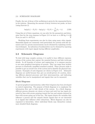
To model the complete system we start with the block diagram in Fig-
ure 3.1. Let v be the speed of the car and vr the desired (reference) speed.
The controller, which typically is of the proportional-integral (PI) type de-
scribed briefly in Chapter 1, receives the signals v and vr and generates a
77

90. 78 CHAPTER 3. EXAMPLES
Gears &
Actuator
vr
Controller
Body
Throttle &
Engine
Fd
v
cancel
resume/accel
set/decel
on/off
Human
Interface
T F
u
Wheels
Figure 3.1: Block diagram of a cruise control system for an automobile.
control signal u that is sent to an actuator that controls throttle position.
The throttle in turn controls the torque T delivered by the engine, which is
then transmitted through gears and the wheels, generating a force F that
moves the car. There are disturbance forces Fd due to variations in the
slope of the road, the effects of rolling resistance and aerodynamic forces.
The cruise controller also has a man-machine interface that allows the driver
to set and modify the desired speed. There are also functions that discon-
nects cruise control when the brake is touched as well as functions to resume
cruise control operation.
The system has many individual components—actuator, engine, trans-
mission, wheels and car body—and a detailed model can be very compli-
cated. In spite of this, the model required to design the cruise controller can
be quite simple. In essence the model should describe how the car’s speed
is influenced by the slope of the road and the control signal u that drives
the throttle actuator.
To model the system, it is natural to start with a momentum balance
for the car body. Let v be the speed measured in m/s, m the total mass of
the car in kg (including passengers), F the force generated by the contact of
the wheels with the road, and Fd the disturbance force due to gravity and
friction. The equation of motion of the car is simply
m
dv
dt
= F − Fd. (3.1)
The force F is generated by the engine, whose torque is proportional to
the rate of fuel injection, which is itself proportional to the control signal
0 ≤ u ≤ 1 that controls throttle position. The torque also depends on engine
speed ω. A simple representation of the torque at full throttle is given by

91. 3.1. CRUISE CONTROL 79
0 200 400 600
100
120
140
160
180
200
Angular velocity (rad/s)
Torque(Nm)
(a)
0 20 40 60
100
120
140
160
180
200
n=1 n=2 n=3 n=4
n=5
Velocity (m/s)
Torque(Nm)
(b)
Figure 3.2: Torque curves for typical car engine: (a) torque as a function of the
angular velocity of the engine and (b) torque as a function of car speed for different
gears.
the torque curve
T(ω) = Tm 1 − β
ω
ωm
− 1
2
, (3.2)
where the maximum torque Tm is obtained at engine speed ωm. Typical
parameters are Tm = 190 Nm, ωm = 420 rad/sec (about 4000 RPM) and
β = 0.4.
Let n be the gear ratio and r the wheel radius. The engine speed is
related to the velocity through the expression
ω =
n
r
v =: αnv,
and the driving force can be written as
F =
nu
r
T(ω) = αnuT(αnv).
Typical values of αn for gears 1 through 5 are α1 = 40, α2 = 25, α3 = 16,
α4 = 12 and α5 = 10. The inverse of αn has physical interpretation as the
effective wheel radius. Figure 3.2 shows the torque as function of engine
speed and vehicle speed. The figure shows that the effect of the gear is
to “flatten” the torque curve so that a torque close to maximum can be
obtained almost over the full speed range.
The disturbance force Fd has three major components: Fg, the forces due
to gravity; Fr, the forces due to rolling friction; and Fa, the aerodynamic

92. 80 CHAPTER 3. EXAMPLES
Fg
mg
F
θ
0 10 20 30
19
19.5
20
20.5
velocity(m/s)
0 10 20 30
0
0.5
1
time (sec)
throttle
(a) (b)
Figure 3.3: Car with cruise control encountering a sloping road: a schematic di-
agram is shown in (a) and (b) shows the response in speed and throttle when a
slope of 4◦
is encountered. The hill is modeled as a net change in hill angle, θ,
of 4 degrees, with a linear change in the angle between t = 5 and t = 6. The PI
controller has proportional gain is kp = 0.5 and the integral gain is ki = 0.1.
drag, Letting the slope of the road be θ, gravity gives the retarding force
Fg = mg sin θ, as illustrated in Figure 3.3a, where g = 9.8 m/sec2 is the
gravitational constant. A simple model of rolling friction is
Fr = mgCr
where Cr is the coefficient of rolling friction; a typical value is Cr = 0.01.
Finally, the aerodynamic drag is proportional to the square of the speed:
Fa =
1
2
ρCdAv2
,
where ρ is the density of air, Cd is the shape-dependent aerodynamic drag
coefficient and A is the frontal area of the car. Typical parameters are
ρ = 1.3 kg/m3, Cd = 0.32 and A = 2.4 m2.
Summarizing, we find that the car can be modeled by
m
dv
dt
= αnuT(αnv) − mgCr − 1
2ρCvAv2
− mg sin θ, (3.3)
where the function T is given by equation (3.2). The model (3.3) is a
dynamical system of first order. The state is the car velocity v, which is also

93. 3.1. CRUISE CONTROL 81
the output. The input is the signal u that controls the throttle position, and
the disturbance is the force Fd, which depends on the slope of the road. The
system is nonlinear because of the torque curve and the nonlinear character
of the aerodynamic drag. There can also be variations in the parameters,
e.g. the mass of the car depends on the number of passengers and the load
being carried in the car.
We add to this model a feedback controller that attempts to regulate
the speed of the car in the presence of disturbances. We shall use a PI
(proportional-integral) controller, which has the form
u(t) = kpe(t) + ki
t
0
e(τ) dτ.
This controller can itself be realized as an input/output dynamical system
by defining a controller state z and implementing the differential equation
dz
dt
= vr − v u = kp(vr − v) + kiz, (3.4)
where vr is the desired (reference) speed. As discussed briefly in the intro-
duction, the integrator (represented by the state z) insures that in steady
state the error will be driven to zero, even when there are disturbances or
modeling errors. (The design of PI controllers is the subject of Chapter 10.)
Figure 3.3b shows the response of the closed loop system, consisting of equa-
tions (3.3) and (3.4), when it encounters a hill. The figure shows that even
if the hill is so steep so that the throttle changes from 0.17 to almost full
throttle, the largest speed error is less than 1 m/s, and the desired velocity
is recovered after 20s.
The model (3.3) is essentially a momentum balance for the car. Many
approximations were made when deriving it. It may be surprising that such
a seemingly complicated system can be described by the simple model (3.3).
As we shall see in later chapters, the reason for this is the inherent robustness
of feedback systems: even if the model is not perfectly accurate, we can use
it to design a controller and make use of the feedback in the controller to
manage the uncertainty in the system.
The cruise control system also has a human-machine interface (HMI)
that allows the driver to communicate with the system. There are many dif-
ferent ways to implement this system; one version is illustrated in Figure 3.4.
The system has four buttons: on-off, set/decelerate, resume/accelerate and
cancel. The operation of the system is governed a finite state system and
which controls the modes of the PI controller and the reference generator.

94. 82 CHAPTER 3. EXAMPLES
Figure 3.4: Finite state machine for cruise control system.
The controller can operate in two ways: in the normal cruise control
mode and in a tracking mode, where the integral is adjusted to match
given process inputs and outputs. The tracking mode is introduced to avoid
switching transients when the system is controlled manually. The generator
for the reference signal has three modes: a normal control mode when the
output is controlled by the set/accelerate and resume/decelerate buttons, a
tracking mode and a hold mode where the reference is held constant.
To control the overall operation of the controller and reference generator,
we use a finite state machine with four states: off, standby, cruise and hold.
The states of the controller and the reference generator in the different modes
are given in Figure 3.4. The cruise mode is the normal operating mode where
the speed can be then be decreased by pushing set/decelerate and increased
by pushing the resume/accelerate. When the system is switched on it goes
to standby mode. The cruise mode is activated by pushing the set/accelerate
button. If the brake is touched or if the gear is changed, the system goes
into hold mode and the current velocity is stored in the reference generator.
The controller is then switched to tracking mode and the reference generator
is switched to hold mode, where it holds the current velocity. Touching the
resume button then switches the system to cruise mode. The system can be
switched to standby mode from any state by pressing the cancel button.
The PI controller should be designed to have good regulation properties
and to give good transient performance when switching between resume
and control modes. Implementation of controllers and reference generators
will be discussed more fully in Chapter 10. A popular description of cruise
control system can be found on the companion web site. Many automotive
applications are discussed in detail in [BP96] and [KN00].

95. 3.2. BICYCLE DYNAMICS 83
ξ
η
η
ζ
a
b
h
δ
ϕ
P1 P2
O
a
b
h
c
C1 C2
P1 P2P3
λ
Figure 3.5: Schematic top (left), rear (middle), and side (right) views of a bicycle.
The steering angle is δ, the roll angle is ϕ. The center of mass has height h and on
the distance a from a vertical through the contact point P1 of the rear wheel. The
wheel base is b and the trail is c.
3.2 Bicycle Dynamics
The bicycle is an interesting dynamical system system with the feature that
one of its key properties is due to a feedback mechanism that is created
by a clever design of the front fork. A detailed model of a bicycle is com-
plex because the system has many degrees of freedom and the geometry is
complicated. However, a great deal of insight can be obtained from simple
models.
To derive the equations of motion we assume that the bicycle rolls on
the horizontal xy plane. Introduce a coordinate system that is fixed to the
bicycle with the ξ-axis through the contact points of the wheels with the
ground, the η-axis horizontal and the ζ-axis vertical, as shown in Figure 3.5.
Let v0 be the velocity of the bicycle at the rear wheel, b the wheel base,
ϕ the tilt angle and δ the steering angle. The coordinate system rotates
around the point O with the angular velocity ω = v0δ/b, and an observer
fixed to the bicycle experiences forces due to the motion of the coordinate
system.
The tilting motion of the bicycle is similar to an inverted pendulum, as
shown in the rear view in Figure 3.5b. To model the tilt, consider the rigid
body obtained when the wheels, the rider and the front fork assembly are
fixed to the rear frame. Let m be the total mass of the system, J the moment
of inertia of this body with respect to the ξ-axis, and D the product of inertia
with respect to the ξζ axes. Furthermore, let the ξ and ζ coordinates of the
center of mass be a and h, respectively. We have J ≈ mh2 and D = mah.

96. 84 CHAPTER 3. EXAMPLES
ϕδ
A
T
Front fork
FrameB
−1
Σ
Figure 3.6: Block diagram of the bicycle with a front fork. The steering torque
applied to the handlebars is T, the roll angle is ϕ, and the steering angle δ. Notice
that the front fork creates a feedback from the roll angle ϕ to the steering angle δ
that under certain conditions can stabilize the system.
The torques acting on the system are due to gravity and centripetal action.
Assuming that the steering angle δ is small, the equation of motion becomes
J
d2ϕ
dt2
−
Dv0
b
dδ
dt
= mgh sin ϕ +
mv2
0h
b
δ, (3.5)
The term mgh sin ϕ is the torque generated by gravity. The terms con-
taining δ and its derivative are the torques generated by steering, with the
term (Dv0/b) dδ/dt due to inertial forces and the term (mv2
0h/b) δ due to
centripetal forces.
The steering angle is influenced by the torque the rider applies to the
handle bar. Because of the tilt of the steering axis and the shape of the front
fork, the contact point of the front wheel with the road P2 is behind the axis
of rotation of the front wheel assembly, as shown in Figure 3.5. The distance
c between the contact point of the front wheel P2 and the projection of the
axis of rotation of the front fork assembly P3 is called the trail. The steering
properties of a bicycle depend critically on the trail. A large trail increases
stability but make the steering less agile.
A consequence of the design of the front fork is that the steering angle δ
is influence both by steering torque T and by the tilt of the frame ϕ. This
means that the bicycle with a front fork is a feedback system as illustrated
by the block diagram in Figure 3.6. The steering angle δ influences the tilt
angle ϕ and the tilt angle influences the steering angle giving rise to the
circular causality that is characteristic for reasoning about feedback. For
a front fork with positive trail, the bicycle will steer into the lean creating

97. 3.3. OPERATIONAL AMPLIFIER 85
a centrifugal force that attempts to diminish the lean. The effect can be
verified experimentally by biking on a straight path, creating a lean by tilting
the body and observing the steering torque required to keep the bicycle
on a straight path when leaning. Under certain conditions, the feedback
can actually stabilize the bicycle. A crude empirical model is obtained by
assuming that the blocks A and B are static gains k1 and k2 respectively:
δ = k1T − k2ϕ. (3.6)
This model neglects the dynamics of the front fork, the tire-road interaction
and the fact that the parameters depend on the velocity. A more accurate
model is obtained by the rigid body dynamics of the front fork and the
frame. Assuming small angles this model becomes
M


¨ϕ
¨δ

 + Cv0


˙ϕ
˙δ

 + (K0 + K2v2
0)


ϕ
δ

 =


0
T

 , (3.7)
where the elements of the 2 × 2 matrices M, C, K0 and K2 depend on
the geometry and the mass distribution of the bicycle. Even this model
is inaccurate because the interaction between tire and road are neglected.
Taking this into account requires two additional state variables.
Interesting presentations of the development of the bicycle are given in
the books by D. Wilson [Wil04] and Herlihy [Her04]. More details on bicycle
modeling is given in the paper [˚AKL05], which has many references. The
model (3.7) was presented in a paper by Whipple in 1899 [Whi99].
3.3 Operational Amplifier
The operational amplifier (op amp) is a modern implementation of Black’s
feedback amplifier. It is a universal component that is widely used for for
instrumentation, control and communication. It is also a key element in
analog computing.
Schematic diagrams of the operational amplifier are shown in Figure 3.7.
The amplifier has one inverting input (v−), one non-inverting input (v+),
and one output (vout). There are also connections for the supply voltages,
e− and e+ and a zero adjustment (offset null). A simple model is obtained
by assuming that the input currents i− and i+ are zero and that the output
is given by the static relation
vout = sat(vmin,vmax) k(v+ − v−) , (3.8)

98. 86 CHAPTER 3. EXAMPLES
(b)
v−
v+
e−
e+
i+
i−
vout
NC
v+
output
offset null
offset null
inverting input
non-inv. input
v−
v+
v− vout
(c)(a)
Figure 3.7: An operational amplifier and two schematic diagrams. The figure on
the left shows the amplifier pin connections on an integrated circuit chip, the middle
figure shows a schematic with all connections, and the diagram on the right shows
only the signal connections.
where sat denotes the saturation function
sat(a,b)(x) =



a if x < a
x if a ≤ x ≤ b
b if x > b.
(3.9)
We assume that the gain k is very large, in the range of 106–108, and the
voltages vmin and vmax satisfy
e− ≤ vmin < vmax ≤ e+
and hence are in the range of the supply voltages. More accurate models
are obtained by replacing the saturation function with a smooth function as
shown in Figure 3.8. For small input signals the amplifier characteristic (3.8)
is linear
vout = k(v+ − v−) =: −kv. (3.10)
vmin
vout
v+ − v−
vmax
Figure 3.8: Input-output characteristics of an operational amplifier.

99. 3.3. OPERATIONAL AMPLIFIER 87
v
−
+
v1
v2
R1 R2
i0
(a) (b)
Figure 3.9: Circuit diagram of a stable amplifier based on negative feedback around
an operational amplifier (a) and the corresponding block diagram (b).
Since the open loop gain k is very large, the range of input signals where
the system is linear is very small.
A simple amplifier is obtained by arranging feedback around the basic
operational amplifier as shown in Figure 3.9a. To model the feedback am-
plifier in the linear range, we assume that the current i0 = i− + i+ is zero,
and that the gain of the amplifier is so large that the voltage v = v− − v+
is also zero. It follows from Ohm’s law that the currents through resistors
R1 and R2 are given by
v1
R1
= −
v2
R2
and hence
v2
v1
= −kcl where kcl =
R2
R1
(3.11)
is the closed loop gain of the amplifier.
A more accurate model is obtained by neglecting the current i0 but
assuming that the voltage v is small but not negligible. The current balance
then becomes
v1 − v
R1
=
v − v2
R2
. (3.12)
Assuming that the amplifier operates in the linear range and using equa-
tion (3.10) the gain of the closed loop system becomes
kcl = −
v2
v1
=
R2
R1
1
1 + 1
k 1 + R2
R1
(3.13)
If the open loop gain k of the operational amplifier is large, the closed loop
gain kcl is the same as in the simple model given by equation (3.11). Notice
that the closed loop gain only depends on the passive components, and
that variations in k only have a marginal effect on the closed loop gain.
For example if k = 106 and R2/R1 = 100, a variation of k by 100% only

100. 88 CHAPTER 3. EXAMPLES
gives a variation of 0.01% in the closed loop gain. The drastic reduction in
sensitivity is a nice illustration of how feedback can be used to make good
systems from bad components. In this particular case, feedback is used
to trade high gain and low robustness for low gain and high robustness.
Equation (3.13) was the formula that inspired Black when he invented the
feedback amplifier.
It is instructive to develop a block diagram for the feedback amplifier in
Figure 3.9a. To do this we will represent the pure amplifier with input v and
output v2 as one block. To complete the block diagram we must describe
how v depends on v1 and v2. Solving equation (3.12) for v gives
v =
R2
R1 + R2
v1 +
R1
R1 + R2
v2 =
R2
R1 + R2
v1 +
R1
R2
,
and we obtain the block diagram shown in Figure 3.9b. The diagram clearly
shows that the system has feedback and that the gain from v2 to v is
R1/(R1 + R2), which can also be read from the circuit diagram in Fig-
ure 3.9a. If the loop is stable and if gain of the amplifier is large it follows
that the error e is small and then we find that v2 = −(R2/R1)v1. Notice
that the resistor R1 appears in two blocks in the block diagram. This situa-
tion is typical in electrical circuits and it is one reason why block diagrams
are not always well suited for some types of physical modeling.
The simple model of the amplifier given by equation (3.10) gives qualita-
tive insight but it neglects the fact that the amplifier is a dynamical system.
A more realistic model is
dvout
dt
= −avout − bv. (3.14)
The parameter b which has dimensions of frequency is called the gain-
bandwidth product of the amplifier.
The operational amplifier is very versatile and many different systems
can be built by combining it with resistors and capacitors. Figure 3.10
shows the circuit diagram for analog PI (proportional-integral) controller.
To develop a simple model for the circuit we assume that the current i0 is
zero and that the open loop gain k is so large that the input voltage v is
negligible. The current i through the capacitor is i = Cdvc/dt, where vc is
the voltage across the capacitor. Since the same current goes through the
resistor R1 we get
i =
v1
R1
= C
dvc
dt
,

101. 3.4. WEB SERVER CONTROL 89
i0
−
+
v1
R1 R2
v2
C
Figure 3.10: Circuit diagram of a PI controller obtained by feedback around an
operational amplifier.
which implies that
vc(t) =
1
C
i(t) dt =
1
R1C
t
0
v1(τ)dτ.
The output voltage is thus given by
v2(t) = −R2i − vc = −
R2
R1
v1(t) −
1
R1C
t
0
v1(τ)dτ,
which is the input/output relation for a PI controller.
The development of operational amplifiers is based on the work of Philbrick [Lun05,
Phi48] and their usage is described in many textbooks (e.g. [CD75]). Very
good information is also available from suppliers [Jun02, Man02].
3.4 Web Server Control
Control is important to ensure proper functioning of web servers, which are
key components of the Internet. A schematic picture of a server is shown
in Figure 3.11. Requests are arriving, queued and processed by the server,
typically on a first-come-first-serve basis. There are typically large variations
in arrival rates and service rates. The queue length builds up when the
messages
x
µλ
message queuemessages
incoming outgoing
Figure 3.11: Schematic diagram of a web server.

102. 90 CHAPTER 3. EXAMPLES
arrival rate is larger than the service rate. When the queue becomes too
large, service is denied using some admission control policy.
The system can be modeled in many different ways. One way is to model
each incoming request, which leads to an event-based model, where the state
is an integer that represents the queue length. The queue changes when a
request arrived or a request is served. A discrete time model that captures
these dynamics is given by the difference equation
xk+1 = xk + ui − uo, x ∈ I
where ui and uo are random variables representing incoming and outgoing
requests on the queue. These variables take on the values 0 or 1 with some
probability at each time instant. To capture the statistics of the arrival and
servicing of messages, we model each of these as a Poisson process in which
the number of events occurring in a fixed time has a given rate, with the
specific timing of events independent of the time since the last event. (The
details of random processes are beyond the scope of this text, but can be
found in standard texts such as [Pit99].)
The system can also described using a flow model by approximating
the requests and services by continuous flows and the queue length by a
continuous variable. A flow model can be obtained by making probabilistic
assumptions on arrival and service rates and computing the average queue
length. For example, assuming that the arrival and service rates are Poisson
processes with intensities λ and µ it can be shown that the average queue
length x is described by the first-order differential equation
dx
dt
= λu − µ
x
x + 1
. (3.15)
The control variable 0 ≤ u ≤ 1 is the fraction of incoming requests that are
serviced, giving an effective arrival rate of uµ. The average time to serve a
request is
Ts =
x
λ
.
If µ, λ and u are constants with µ > uλ, the queue length x approaches the
steady state value
xss =
uλ
µ − uλ
. (3.16)
Figure 3.12a shows the steady state queue length as a function of µ−uλ, the
effective service rate excess. Notice that the queue length increases rapidly
as µ − uλ approaches zero. To have a queue length less than 20 requires
µ > uλ + 0.05.

103. 3.4. WEB SERVER CONTROL 91
0 0.2 0.4 0.6 0.8 1
0
50
100
µ − uλ
x
(a)
0 20 40 60 80
0
5
10
15
20
t
µ−uλ
(b)
Figure 3.12: The figure on the left shows steady state queue length as a function
of uλ − µ, and the figure on the right shows the behavior of the queue length
when there is a temporary overload in the system. The full line shows a realization
of an event based simulation and the dashed line shows the behavior of the flow
model (3.15).
Figure 3.12b illustrates the behavior of the server in a typical overload
situation. The service rate is µ = 1, while the arrival rate starts at λ = 0.5.
The arrival rate is increased to λ = 4 at time 20, and it returns to λ = 0.5 at
time 25. The figure shows that the queue builds up quickly and clears very
slowly. Since the response time is proportional to queue length, it means
that the quality of service is poor for a long period after an overload. The
behavior illustrated in Figure 3.12b, which is called the rush-hour effect,
has been observed in web servers and in many other queuing systems like
automobile traffic. Congestion avoidance is a main reason for controlling
queues.
The dashed line in Figure 3.12b shows the behavior of the flow model,
which describes the average queue length. The simple model captures be-
havior qualitatively, but since the queue length is short there is significant
variability from sample to sample. The behavior shown in Figure 3.12b can
be explained quantitatively by observing that the queue length increases
at constant rate over large time intervals. It follows from equation (3.15)
that the rate of change is approximately 3 messages/second when the queue
length builds up at time t = 20, and approximately 0.5 messages/second
when the queue length decreases after the build up. The time to return to
normal is thus approximately 6 times the overload time.
Admission Control
The long delays created by temporary overloads can be reduced by access
control. The queue length can be controlled by only admitting a fraction of
the incoming requests. Figure 3.13 shows what happens when a simple ad-

104. 92 CHAPTER 3. EXAMPLES
0 20 40 60 80
0
0.5
1
1.5
2
0 20 40 60 80
0
0.5
1
xu
t
(a) r = 2
0 20 40 60 80
0
2
4
6
0 20 40 60 80
0
0.5
1
x
u
t
(b) r = 5
Figure 3.13: Behavior of queue length for a server with admission control when
there is a temporary overload in the system. The figure on the left has r = 2 and
the right figure has r = 5, with k = 1 in both cases. Compare with a simulation of
the uncontrolled system in Figure 3.12b.
mission control strategy is introduced. The feedback used in the simulation
is a simple proportional control with saturation described by
u = sat(0,1)(k(r − x)), (3.17)
where sat(a,b) is defined in equation (3.9) and r is the desired (reference)
queue length. The feedback gain is k = 1, and the saturation ensures that
the control variable is in the interval 0 ≤ u ≤ 1. Comparing Figures 3.12b
and 3.13, we see that simple access control works very well in comparison
with the uncontrolled server. The control law ensures that the access is
restricted when overload occurs.
The maximum queue length is determined by the reference value r. A
low value of r gives a short queue length and the service delay is short,
as is clearly seen in Figure 3.13a. A number of customers are, however,
denied service. The simulation also indicates that the control problem is
not too difficult and that a simple control strategy works quite well. It
allows all requests arrived to be serviced if the arrival rate is slow and it
restricts admission when the system is overloaded. Admission control is
activated when the queue length approaches the value r. Since service time
is proportional to queue length, r is a measure of service time.
Notice that the web server control problem we have discussed is not a
conventional regulation problem where we wish to keep a constant queue

105. 3.4. WEB SERVER CONTROL 93
length. The problem is instead to make sure that the queue length does not
become too large when there are many service requests. The key trade-off
is to find a good reference value r. A large value gives few rejections but
long service time after an overload; a small value guarantees a short service
time but more messages will be rejected. The simulation of the simple flow
model indicates that the simple admission control strategy works well.
To execute admission control in a real queue, where arrival and departure
from the queue are discrete events, we argue as follows. Figure 3.13 shows
that all requests are serviced (u = 1) except when the system is overloaded,
at which point service is reduced significantly. A simple strategy that mimics
this for event-based systems is to admit customers as long as the queue
length is less than r and deny service for requests if the queue length is
greater than r.
Delay Control
An alternative to admission control is delay control, where the goal is to
keep the delay for serving individual requests constant. An advantage of
this approach is that all requests are treated fairly. A block diagram of such
a system, with a controller combining feedback ufb and feedforward uff, is
shown in Figure 3.14a. The server delay is estimated based on arriving server
requests and queue waiting times of requests that have not been serviced.
Feedforward control requires good models and the simple model (3.15) that
captures the average behavior of the system is not sufficient.
The control variable is the processing speed u, which can be varied by the
changing the number of servers and their processing capacity. It is assumed
that u can be regarded as a continuous variable. The delays in serving the
requests is the output of the system. An average of past service is easily
obtained, but this information is only available with a time delay.
To obtain a better model we consider the situation in Figure 3.14b. A
request has just been serviced at time t = tk and N requests are waiting
to be serviced. The average delay of the N requests that are waiting to be
serviced is d−
k , which is a measurable quantity. To predict the additional
time required to serve these request we assume that they require the same
service time C/u where u is the service rate. The average additional service
time for the requests that are processed is then d+
k = (N + 1)C/(2u), as
indicated in Figure 3.14b. Combining this with the measurable quantity
d−
k we obtain the following estimate of the average service time for the N

106. 94 CHAPTER 3. EXAMPLES
(a) (b)
Figure 3.14: The left figure (a) shows a block diagram of a web server system with
a controller based on a combination of feedback and feedforward. The right figure
(b) shows the history of arrivals and departures of requests. The dashed square
indicates the time used to service the requests. The true delay of the request
serviced at time tk is dk, d−
k + d+
k is an estimate of future delays used to calculate
the service rate.
requests that are waiting to be serviced
dk = d−
k + d+
k = d−
k +
(N + 1)C
2u
.
Requiring that dk is equal to the desired delay time dr, we find that the
service rate at instant k should be chosen as
uk =
(N + 1)C
2(dr − d−
k )
, (3.18)
which is the formula used to calculate the feedforward control signal at time
tk. The control action can recalculated at each time instant, resulting in
a control strategy called receding horizon control. The choice of recalcula-
tion rate is a compromise because frequent recalculations improves control
quality but it also consumes computer resources.
The feedforward is complemented with a feedback controller in the form
of a PI controller based on the measured delay at event k. Since the queue
dynamics varies with the delay time it is useful to let the parameters of the
PI controller depend on the desired delay dr, an example of gain scheduling.
The control algorithm has been tested experimentally on a testbed of
PC’s connected via Ethernet. One PC was was assigned to run the web
server, and the others were generating a synthetic workload. The goal of
the system was to provide the delay guarantee for that class with as few
resources as possible. The input load patterns generated by the clients are

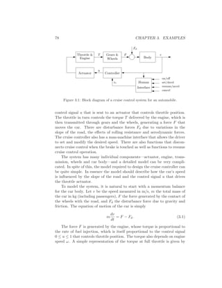
107. 3.5. ATOMIC FORCE MICROSCOPE 95
Figure 3.15: Arrival rate (top) and average service delay (bottom) for an experiment
with web server control (from [HLA04]).
shown in Figure 3.15. The desired delay for the class was set to dr = 4s in all
experiments. The figure shows that the control algorithm keeps the service
time reasonably constant and that the PI controller reduces the variations
in delay compared with a pure feedforward controller.
This example illustrates that simple models can give good insight and
that nonlinear control strategies are useful. The example also illustrates
that continuous time models can be useful for phenomena that are basically
discrete. There are also converse examples. Therefore it is a good idea to
keep an open mind and master both discrete and continuous time modeling.
The book by Hellerstein et al. [HDPT04] gives many examples of use of
feedback in computer systems. The example on delay control is based on
the work of Henriksson [HLA04, Hen06].
3.5 Atomic Force Microscope
The 1986 Nobel Prize in Physics was shared by Gerd Binnig and Heinrich
Rohrer for their design of the scanning tunneling microscope (SCM). The
idea of an SCM is to bring an atomically sharp tip so close to a conducting
surface that tunneling occurs. An image is obtained by traversing the tip
and measuring the tunneling current as a function of tip position. The
image reflects the electron structure of the upper atom-layers of the sample.

108. 96 CHAPTER 3. EXAMPLES
(a) (b)
Figure 3.16: Schematic diagram of an atomic force microscope and a sample AFM
image of DNA.
This invention has stimulated development of a family of instruments that
permit visualization of surface structure at the nanometer scale, including
the atomic force microscope (AFM). These instruments are now standard
tools for exploring nanoscale structures.
In the atomic force microscope, a sample is probed by a tip on a cantilever
which is controlled to exert a constant force on the sample. The control
system is essential because it has a direct influence on picture quality and
scanning rate. Since the dynamic behavior of the system changes with the
properties of the sample, it is necessary to tune the feedback loop, which is
currently done manually by adjusting parameters of a PI controller. There
are interesting possibilities to make the systems easier to use by introducing
automatic tuning and adaptation.
A schematic picture of an atomic force microscope is shown in Fig-
ure 3.16a. A micro-cantilever with a tip having a radius of the order of
10 nm is placed close to the sample. The tip can be moved vertically and
horizontally using a piezoelectric scanner. Atomic forces bend the cantilever
and the cantilever tilt is measured by sensing the deflection of the beam us-
ing a photo diode. The signal from the photo diode is amplified and sent
to a controller that drives the amplifier for the vertical deflection of the
cantilever. By controlling the piezo scanner so that the deflection of the
cantilever is constant, the signal driving the vertical deflection of the scan-
ner is a measure of the atomic forces between the cantilever tip and the
atoms of the sample. An image of the surface is obtained by scanning the
cantilever along the sample. The resolution makes it possible to see the
structure of the sample on the atomic scale, as illustrated in Figure 3.16b,

109. 3.5. ATOMIC FORCE MICROSCOPE 97
Figure 3.17: Block diagram of the system for vertical positioning of the cantilever.
which shows an AFM image of DNA.
To model the system, we start with the block diagram shown in Fig-
ure 3.17, which shows the major components. Signals that are easily acces-
sible are: the voltage Vp that drives the piezo scanner, the input voltage u
to its power amplifier and the output voltage y of the signal amplifier for
the photo diode. The controller is a PI controller implemented by a com-
puter, which is connected to the system by A/D and D/A converters. The
deflection of the cantilever, ϕ, is also shown.
For a more detailed model we will start with the cantilever, which is at
the heart of the system. The micro-cantilever is modeled as a spring-mass-
damper system. Let z be the distance from the tip of the cantilever to the
sample and let v be the position of the cantilever base. Furthermore let m,
k and c be the effective values of mass, spring and damping coefficients. The
equation of motion of the cantilever is then
m
d2z
dt2
+ c
dz
dt
+ k(z − v) = F, (3.19)
where F is the atomic force between the sample and the cantilever tip.
Neutral atoms and molecules are subject to two forces, an attractive van
der Waals force, and a repulsion force due to the Pauli exclusion princi-
ple. The force between two atoms can be approximately described by the
Lennard-Jones potential given by
VLJ (z) = A
σ
z
12
−
σ
z
6
,
where σ is the atom radius and r the distance between the atoms. Ap-
proximating the cantilever tip by a sphere with radius R and the sample by
a flat surface then integrating the Lennard-Jones potential, the interaction

110. 98 CHAPTER 3. EXAMPLES
(a) (b)
Figure 3.18: Measured step response and model of piezo scanner. The left figure
shows a measured step response. The blue signal shows the input is the voltage
applied to the drive amplifier (50 mV/div), the red curve is the output of the power
amplifier (500 mV/div) and the red curve is the output of the signal amplifier (500
mV/div). The time scale is 25 µs/div. The right figure is a simple mechanical
model for the vertical positioner and the piezo crystal.
between the cantilever and the sample can be described by the following
potential
V (z) =
HR
6σ
1
120
σ
z
7
−
σ
z
,
where H ≈ 10−19 J is the Hamaker constant, and a typical atom radius
is σ = 0.4 nm. The potential has a minimum where the distance between
the tip is less than an atom size from the sample and the tip is essentially
clamped at the minimum by the atomic forces. The natural frequency of
the clamped cantilever is so high that the dynamics of the cantilever can
be neglected and we can model the cantilever as a static system. For small
deviations, the bending ϕ of the cantilever is then proportional to the vertical
translation of the cantilever.
The piezo scanner gives a deflection that is proportional to the applied
voltage, but the system and the amplifiers also have dynamics. Figure 3.18a
shows a step response of a scanner from the input voltage u to the drive
amplifier to the output voltage y of the signal amplifier for the photo diode.
A schematic mechanical representation of the vertical motion of the scanner
is shown in Figure 3.18b. The figure shows that the system responds quickly
but that there is a poorly damped oscillatory mode caused by the dynamics
of the scanner. The instrument designer has two choices, either to accept
the oscillation and to have a slow response time or else to design a control

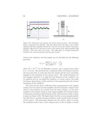
111. 3.6. DRUG ADMINISTRATION 99
system that can damp the oscillations which gives a faster response and a
faster imaging. Damping the oscillations is a significant challenge because
there are many oscillatory modes and they can change depending on how the
instrument is used. An instrument designer also has the choice to redesign
the mechanics so that the resonances occur at higher frequencies.
The book by Sarid [Sar91] gives a broad coverage of atomic force micro-
scopes. The interaction of atoms close to surfaces is fundamental to solid
state physics. A good source is Kittel [Kit95] where the Lennard-Jones po-
tential is discussed. Modeling and control of atomic force microscopes are
discussed by Schitter [Sch01].
3.6 Drug Administration
The phrase “take two pills three times a day” is a recommendation that we
are all familiar with. Behind this recommendation is a solution of an open
loop control problem. The key issue is to make sure that the concentration
of a medicine in a part of our bodies will be sufficiently high to be effective
but not so high that it will cause undesirable side effects. The control action
is quantized, take two pills, and sampled, every 8 hours. The prescriptions
can be based on very simple models in terms of empirical tables where the
dosage is based on the age and weight of the patient. A more sophisticated
administration of medicine is used to keep concentration of insulin and glu-
cose at a right level. In this case the substances are controlled by continuous
measurement and injection, and the control schemes are often model based.
Drug administration is clearly a control problem. To do it properly it
is necessary to understand how a drug spreads in the body after it is ad-
ministered. This topic, called pharmacokinetics, is now its own discipline
and the models used are called compartment models. They go back to 1920
when Widmark modeled propagation of alcohol in the body [WT24]. Phar-
macokinetics describes how drugs are distributed in different organs of the
body. Compartment models are now important for screening of all drugs
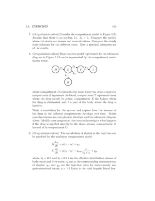
used by humans. The schematic diagram in Figure 3.19 illustrates the idea
of a compartment model. Compartment models are also used in many other
fields such as environmental science.
One-Compartment Model
The simplest dynamic model is obtained by assuming that the body behaves
like a single compartment: that the drug is spread evenly in the body after

112. 100 CHAPTER 3. EXAMPLES
Figure 3.19: Schematic diagram of the circulation system (from Teorell [Teo37]).
it has been administered, and that it is then removed at a rate proportional
to the concentration. Let c be the concentration, V the volume and q the
outflow rate or the clearance. Converting the description of the system into
differential equations, the model becomes
V
dc
dt
= −qc. (3.20)
This equation has the solution
c(t) = c0e−qt/V
= c0e−kt
,
which shows that the concentration decays exponentially after an injection.
The input is introduced implicitly as an initial condition in the model (3.20).
The way the input enters the model depends on how the drug is adminis-
tered. The input can be represented as a mass flow into the compartment
where the drug is injected. A pill that is dissolved can also be interpreted
as an input in terms of a mass flow rate.
The model (3.20) is called a a one-compartment model or a single pool
model. The parameter q/V is called the elimination rate constant. The
simple model is often used in studies where the concentration is measured
in the blood plasma. By measuring the concentration at a few times, the
initial concentration can be obtained by extrapolation. If the total amount
of injected substance is known, the volume V can then be determined as
V = m/c0; this volume is called the the apparent volume of distribution.
This volume is larger than the real volume if the concentration in the plasma
is lower than in other parts of the body. The model (3.20) is very simple
and there are large individual variations in the parameters. The parameters
V and q are often normalized by dividing with the weight of the person.

113. 3.6. DRUG ADMINISTRATION 101
V1 V2
u
k1
k2
k0
Figure 3.20: Schematic diagram of a model with two compartments.
Typical parameters for aspirin are V = 0.2 l/kg and q = 0.01 l/h/kg. These
numbers can be compared with a blood volume of 0.07 l/kg, a plasma volume
of 0.05 l/kg and intracellular fluid volume of 0.4 l/kg.
The simple one compartment model gives the gross behavior but it is
based on strong simplifications. Improved models can be obtained by con-
sidering the body as composed of several compartments. We will work out
the details for a system with two compartments.
Two-Compartment Model
Consider the system shown in Figure 3.20, where the compartments are
represented as circles and the flows by arrows. We assume that there is
perfect mixing in each compartment and that the transport between the
compartments are driven by concentration differences. We further assume
that a drug with concentration c0 is injected in compartment 1 at a volume
flow rate of u and that the concentration in compartment 2 is the output.
Let x1 and x2 be the total mass of the drug in the compartments and
let V1 and V2 be the volumes of the compartments. A mass balance for the
system gives
dx1
dt
= q(c2 − c1) − q0c1 + c0u = q
x2
V2
−
x1
V1
−
q0
V1
c1 + c0u
= −(k1 + k0)x1 + k2x2 + c0u
dx2
dt
= q(c1 − c2) = q
x1
V1
−
x2
V2
= k1x1 − k2x2
y = c2 =
1
V2
x2,
where k0 = q0/V1, k1 = q/V1 and k2 = q/V2. Introducing matrices, this

114. 102 CHAPTER 3. EXAMPLES
model can be written as
dx
dt
=


−k0 − k1 k2
k1 −k2

 x +


c0
0

 u
y =

0 1/V2

 x.
(3.21)
In this model we have used the total mass of the drug in each compartment
as state variables. If we instead choose to use the concentrations as state
variables, the model becomes
dc
dt
=


−k0 − k1 k1
k2 −k2

 c +


b0
0

 u
y =

0 1

 x,
(3.22)
where b0 = c0/V1. Mass is called an extensive variable and concentration is
called an intensive variable.
The papers by Widmark and Tandberg [WT24] and Teorell [Teo37] are
classics. Pharmacokinetics is now an established discipline with many text-
books [Dos68, Jac72, GP82]. Because of its medical importance pharmacoki-
netics is now an essential component of drug development. Compartment
models are also used in other branches of medicine and in ecology. The
problem of determining rate coefficients from experimental data is discussed
in [B˚A70] and [God83].
3.7 Population Dynamics
Population growth is a complex dynamic process that involves the interac-
tion of one or more species with their environment and the larger ecosystem.
The dynamics of population groups are interesting and important in many
different areas of social and environmental policy. There are examples where
new species have been introduced in new habitats, sometimes with disas-
trous results. There are also been attempts to control population growth
both through incentives and through legislation. In this section we describe
some of the models that can be used to understand how populations evolve
with time and as a function of their environment.
Simple Growth Model
Let x the the population of a species at time t. A simple model is to assume
that the birth and death rates are proportional to the total population. This

115. 3.7. POPULATION DYNAMICS 103
gives the linear model
dx
dt
= bx − dx = (b − d)x = rx (3.23)
where birth rate b and death rate d are parameters. The model gives an
exponential increase if b > d or an exponential decrease if B < d. A more
realistic model is to assume that the birth rate decreases when the pop-
ulation is large. The following modification of the model (3.23) has this
property:
dx
dt
= rx(1 −
x
xc
) = f(x), (3.24)
where xc is the carrying capacity of the environment. The model (3.24) is
called the logistic growth model.
Predator Prey Models
A more sophisticated model of population dynamics includes the effects
of competing populations, where one species may feed on another. This
situation, referred to as the predator prey problem, was already introduced
in Example 2.3, where we developed a discrete time model that captured
some of the features of historical records of lynx and hare populations.
In this section, we replace the difference equation model used there with
a more sophisticated differential equation model. Let H(t) represent the
number of hares (prey) and L(t) represent the number of lynxes (predator).
The dynamics of the system are modeled as
dH
dt
= rhH 1 −
H
K
−
aHL
1 + aHTh
H ≥ 0
dL
dt
= rlL 1 −
L
kH
L ≥ 0.
In the first equation, rh represents the growth rate of the hares, K represents
the maximum population of hares (in the absence of lynxes), a represents
the interaction term that describes how the hares are diminished as a func-
tion of the lynx population, and Th depends is a time constant for prey
consumption. In the second equation, rl represents the growth rate of the
lynxes and k represents the fraction of hares versus lynxes at equilibrium.
Note that both the hare and lynx dynamics include terms that resemble the
logistic growth model (3.24).
Of particular interest are the values at which the population values re-
main constant, called equilibrium points. The equilibrium points for this

116. 104 CHAPTER 3. EXAMPLES
0 10 20 30 40 50 60 70 80 90
0
50
100
150
200
250
Time (years)
Population
Hare
Lynx
Figure 3.21: A simulation of the predator prey model with rh = 0.02, K = 500,
a = 0.03, Th = 5, rl = 0.01, k = 0.2 and time scale chosen to correspond to weeks.
system can be determined by setting the right hand side of the above equa-
tions to zero. Letting He and Le represent the equilibrium state, from the
second equation we have
Le = kHe.
Substituting this into the first equation, we must solve
rhHe 1 −
He
K
−
akH2
e
1 + aHeTh
= 0.
Multiplying through by the denominator, we get
0 = He ó rh 1 −
He
K
(1 + aHeTh) − akHe
= He ó
rhaTh
K
H2
e + (ak + rh/K − rhaTh)He − rh .
This gives one solution at He = 0 and a second that can be solved analyti-
cally or numerically.
Figure 3.21 shows a simulation of the dynamics starting from a set of
population values near the nonzero equilibrium values. We see that for this
choice of parameters, the simulation predicts an oscillatory population count
for each species, reminiscent of the data shown in Figure 2.6 (page 48).
Fisheries Management
We end this section by discussing a control problem that has had significant
impact on international legislation for fishing.
The dynamics of a commercial fishery can be described by the following
simple model
dx
dt
= f(x) − h(x, u), (3.25)

117. 3.7. POPULATION DYNAMICS 105
where x be the total biomass, f(x) the growth rate and h(x, u) the harvesting
rate. The logistic function (3.24) is a simple model for the growth rate and
the harvesting can be modeled by
h(x, u) = axu, (3.26)
where the control variable u is the harvesting effort, and a is a constant.
The rate of revenue is
g(x, u) = bh(x, u) − cu, (3.27)
where b and c are constants representing the price of fish and the cost of
fishing. Using equations (3.26) and (3.27) we find that the rate of revenue
is
g(x, u) = (abx − c)u.
In a situation where there are many fishermen and no concern for the envi-
ronment, it is economic to fish as long as abx > c and there will then be an
equilibrium where the biomass is
x∞ =
c
ab
, (3.28)
which is the equilibrium with unrestricted fishing.
Assume that the population is initially at equilibrium at x(0) = xc. The
revenue rate with unrestricted fishing is then (abxc −c)u, which can be very
large. The fishing effort then naturally increases until the equilibrium (3.28),
where the revenue rate is zero.
We can contrast unrestricted fishing with the situation for a single fish-
ery. A typical case is when a country has all fishing rights in a large area.
In such a case it is natural to maximize the rate of sustainable revenue.
This can be accomplished by adding the constraint that the biomass x in
equation (3.25) is constant, which implies that
f(x) = h(x, u).
Solving this equation for u gives
u = ud(x) =
f(x)
ax
.
Inserting the value of u into equation (3.27) gives the following rate of rev-
enue
g(x) = bh(x, ud) − cud(x) = b −
c
ax
f(x)
= rx b −
c
ax
1 −
x
xc
=
r
xc
−abx2
+ (c + abxc)x − cxc .
(3.29)

118. 106 CHAPTER 3. EXAMPLES
0 5 10 15 20 25 30 35 40 45 50
0
50
100
0 5 10 15 20 25 30 35 40 45 50
0
2
4
0 5 10 15 20 25 30 35 40 45 50
0
10
20
30
x
ug
t
Figure 3.22: Simulation of a fishery. The curves show total biomass x, harvesting
rate u and revenue rate g as a function of time t. The fishery is modeled by
equations (3.25), (3.26), (3.27) with parameters xc = 100, a = 0.1, b = 1 and c = 1.
Initially fishing is unrestricted at rate u = 3, at time t = 15 fishing is changed to
harvesting at a sustainable rate, accomplished by a PI controller with parameters
k = 0.5 and ki = 0.5.
The rate of revenue has a maximum
r0 =
r(c − abxc)2
4abxc
, (3.30)
for
x0 =
xc
2
+
c
2ab
. (3.31)
Figure 3.22 shows a simulation of a fishery. The system is initially in equi-
librium with x = 100. Fishing begins with constant harvesting rate u = 3
at time t = 0. The initial revenue rate is large, but it drops rapidly as the
population decreases. At time t = 12 the revenue rate is practically zero.
The fishing policy is changed to a sustainable strategy at time t = 15. This
is accomplished by using a PI controller where the reference is the optimal
sustainable population size x0 = 55, given by equation (3.31). The feedback
stops harvesting for a period but the biomass increases rapidly. At time
t = 28 the harvesting rate increases rapidly and a sustainable steady state
is reached in a short time.
Volume I of the two volume set by J. Murray [Mur04] give a broad
coverage of population dynamics. Maintaining a sustainable fish population

119. 3.8. EXERCISES 107
is a global problem that has created many controversies and conflicts. A
detailed mathematical treatment is given in [?]. The mathematical analyses
has influenced international agreement on fishing.
3.8 Exercises
1. Consider the cruise control example described in Section 3.1. Build a
simulation that recreates the response to a hill shown in Figure 3.3b
and show the effects of increasing and decreasing the mass of the car
by 25%. Redesign the controller (using trail and error is fine) so that
it returns to the within 10% of the desired speed within 3 seconds of
encountering the beginning of the hill.
2. Consider the inverted pendulum model of the bicycle given in Fig-
ure 3.6. Assume that the block labeled body is modeled by equa-
tion (3.5) and that the front fork is modeled by (3.6). Derive the
equations for the closed loop. Show that when T = 0 the equation
is the same as for a mass spring damper system. Also show that
the spring coefficient is negative for low velocities but positive if the
velocity is sufficiently large.
3. Show that the dynamics of a bicycle frame given by equation (3.5) can
be written in state space form as
d
dt


x1
x2

 =


0 mgh/J
1 0




x1
x2

 +


1
0

 u
y =

Dv0
bJ
mv2
0h
bJ

 x,
where the input u is the torque applied to the handle bars and the
output y is the title angle ϕ. What do the states x1 and x2 represent?
4. Combine the bicycle model given by equation (3.5) and the model for
steering kinematics in Example 2.8 to obtain a model that describes
the path of the center of mass of the bicycle.
5. Consider the op amp circuit shown below:

120. 108 CHAPTER 3. EXAMPLES
v2
−
+
Rb
v1
v3
R1 Ra
R2
C2
C1
vo
Show that the dynamics can be written in state space form as
dx
dt
=


− 1
R1C1
− 1
RaC1
0
Rb
Ra
1
R2C2
− 1
R2C2

 x +


1
R1C1
0

 u
y =

0 1

 x
where u = v1 and y = v3. (Hint: Use v2 and v3 as your state variables.)
6. (Atomic force microscope) A simple model for the vertical motion of
the scanner is shown in Figure 3.18b, where the system is approxi-
mated with two masses. The mass m1 is half of the piezo crystal and
the mass m2 is the other half of the piezo crystal and the mass of
the support. A simple model is obtained by assuming that the piezo
crystal generates a force F between the masses and that there is a
damping c in the spring. Let the positions of the center of the masses
be x1 and x2, and let the elongation of the piezo stack is u = x1 − x2.
A momentum balance gives the following model for the system.
m1
d2x1
dt2
= F
m2
d2x2
dt2
= −c
dx2
dt
− kx2 − F
u = x1 − x2.
Review the assumptions made in the simplified model. Let the elon-
gation u of the piezo stack be the control variable and the height of
the sample x1 be the output. Show that the relation between x1 and
u is given by
(m2 − m1)
d2x1
dt2
+ c
dx1
dt
+ kx1 = m1
d2u
dt2
+ c
du
dt
+ ku.
Simulate the system and show that the response is qualitatively the
same as the one shown in Figure 3.18a. Can the parameters of the
model be determined from a step response experiment of the type
shown in Figure 3.18a?

121. 3.8. EXERCISES 109
7. (Drug administration) Consider the compartment model in Figure 3.20.
Assume that there is no outflux, i.e. k0 = 0. Compare the models
where the states are masses and concentrations. Compute the steady
state solutions for the different cases. Give a physical interpretation
of the results.
8. (Drug administration) Show that the model represented by the schematic
diagram in Figure 3.19 can be represented by the compartment model
shown below:
D B T I
K
k1
k2
k3
k4
k5
where compartment D represents the issue where the drug is injected,
compartment B represents the blood, compartment T represents tissue
where the drug should be active, compartment K the kidney where
the drug is eliminated, and I a part of the body where the drug is
inactive.
Write a simulation for the system and explore how the amount of
the drug in the different compartments develops over time. Relate
you observations to your physical intuition and the schematic diagram
above. Modify your program so that you can investigate what happens
if the drug is injected directly to the blood stream, compartment B,
instead of in compartment D.
9. (Drug administration) The metabolism of alcohol in the body has can
be modeled by the nonlinear compartment model
Vb
dcb
dt
= q(cl − cb) + qiv
Vl
dcl
dt
= q(cb − cl) − qmax
cl
c0 + cl
+ qgi
where Vb = 48 l and Vl = 0.6 l are the effective distribution volume of
body water and liver water, cb and cl the corresponding concentrations
of alcohol, qiv and qgi are the injection rates for intravenously and
gastrointestinal intake, q = 1.5 l/min is the total hepatic blood flow,

122. 110 CHAPTER 3. EXAMPLES
qmax = 2.75 mmol/min and km = 0.1 mmol. Simulate the system and
compute the concentration in the blood for oral and intravenous doses
of 12 g and 40 g of alcohol.
10. (Population dynamics) Consider the model for logistic growth given
by equation (3.24). Show that the maximum growth rate occurs when
the size of the population is half of the steady state value.
11. (Population dynamics) Verify the curves in Figure 3.21 by creating a
program that integrates the differential equations.

123. Chapter 4
Dynamic Behavior
Predictability: Does the Flap of a Butterfly’s Wings in Brazil set off a Tor-
nado in Texas?
Talk given by Edward Lorenz, December 1972 meeting of the American As-
sociation for the Advancement of Science.
In this chapter we give a broad discussion of the behavior of dynamical
systems, focused on systems modeled by nonlinear differential equations.
This allows us to discuss equilibrium points, stability, limit cycles and other
key concepts of dynamical systems. We also introduce some methods for
analyzing global behavior of solutions.
4.1 Solving Differential Equations
In the last chapter, we saw that one of the methods of modeling dynamical
systems is through the use of ordinary differential equations (ODEs). A
state space, input/output system has the form
dx
dt
= f(x, u)
y = h(x, u),
(4.1)
where x = (x1, . . . , xn) ∈ Rn is the state, u ∈ Rp is the input, and y ∈ Rq
is the output. The smooth maps f : Rn × Rp → Rn and h : Rn × Rp → Rq
represent the dynamics and measurements for the system. We will focus in
this text on single input, single output (SISO) systems, for which p = q = 1.
We begin by investigating systems in which the input has been set to a
function of the state, u = α(x). This is one of the simplest types of feedback,
111

124. 112 CHAPTER 4. DYNAMIC BEHAVIOR
in which the system regulates its own behavior. The differential equations
in this case become
dx
dt
= f(x, α(x)) = F(x). (4.2)
In order to understand the dynamic behavior of this system, we need to
analyze the features of the solutions of equation (4.2). While in some simple
situations we can write down the solutions in analytical form, more often we
must rely on computational approaches. We begin by describing the class
of solutions for this problem.
Initial Value Problems
We say that x(t) is a solution of the differential equation (4.2) on the time
interval t0 ∈ R to tf ∈ R if
dx(t)
dt
= F(x(t)) for all t0 ≤ t ≤ tf .
A given differential equation may have many solutions. We will most often
be interested in the initial value problem, where x(t) is prescribed at a given
time t0 ∈ R and we wish to find a solution valid for all future time, t > t0.
We say that x(t) is a solution of the differential equation (4.2) with initial
value x0 ∈ Rn at t0 ∈ R if
x(t0) = x0 and
dx(t)
dt
= F(x(t)) for all t0 ≤ t ≤ tf .
For most differential equations we will encounter, there is a unique solution
that is defined for t0 ≤ t ≤ tf . The solution may defined for all time t ≥ t0,
in which case we take tf = ∞. Because we will primarily be interested in
solutions of the initial value problem for ODEs, we will often refer to this
simply as the solution of an ODE.
We will usually assume that t0 is equal to 0. In the case when F is inde-
pendent of time (as in equation (4.2)), we can do so without loss of generality
by choosing a new independent (time) variable, τ = t − t0 (Exercise 2).
Example 4.1 (Damped oscillator). Consider a damped, linear oscillator,
introduced in Example 2.4. The equations of motion for the system are
m¨q + c ˙q + kq = 0,
where q is the displacement of the oscillator from its rest position. We
assume that c2 < 4km, corresponding to a lightly damped system (the

125. 4.1. SOLVING DIFFERENTIAL EQUATIONS 113
0 2 4 6 8 10 12 14 16 18 20
−1
−0.5
0
0.5
1
time (sec)
x
1
,x
2
x
1
x
2
Figure 4.1: Response of the damped oscillator to the initial condition x0 = (1, 0).
reason for this particular choice will become clear later). We can rewrite
this in state space form by setting x1 = q and x2 = ˙q, giving
˙x1 = x2
˙x2 = −
k
m
x1 −
c
m
x2.
In vector form, the right hand side can be written as
F(x) =


x2
− k
mx1 − c
mx2

 .
The solution to the initial value problem can be written in a number of
different ways and will be explored in more detail in Chapter 5. Here we
simply assert that the solution can be written as
x1(t) = e− ct
2m x10 cos ωdt +
cx10 + 2mx20
2mωd
sin ωdt
x2(t) = e− ct
2m x20 cos ωdt −
2kx10 + cx20
2mωd
sin ωdt ,
where x0 = (x10, x20) is the initial condition and ωd =
√
4km − c2/2m. This
solution can be verified by substituting it into the differential equation. We
see that the solution is explicitly dependent on the initial condition and it
can be shown that this solution is unique. A plot of the initial condition
response is shown in Figure 4.1. We note that this form of the solution only
holds for c2 − 4km < 0, corresponding to an “underdamped” oscillator. ∇

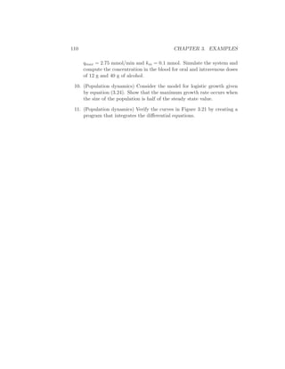
126. 114 CHAPTER 4. DYNAMIC BEHAVIOR
Numerical Solutions
One of the benefits of the computer revolution that is that it is very easy
to obtain a numerical solution of a differential equation when the initial
condition is given. A nice consequence of this is as soon as we have a model
in the form of equation (4.2), it is straightforward to generate the behavior
of x for different initial conditions, as we saw briefly in the previous chapter.
Modern computing environments such as LabVIEW, MATLAB and Math-
ematica allow simulation of differential equations as a basic operation. For
example, these packages provides several tools for representing, simulating,
and analyzing ordinary differential equations of the form in equation (4.2).
To define an ODE in MATLAB or LabVIEW, we define a function repre-
senting the right hand side of equation (4.2):
function xdot = system(t, x)
xdot(1) = F1(x);
xdot(2) = F2(x);
...
Each expression Fi(x) takes a (column) vector x and returns the ith el-
ement of the differential equation. The second argument to the function
system, t, represents the current time and allows for the possibility of time-
varying differential equations, in which the right hand side of the ODE in
equation (4.2) depends explicitly on time.
ODEs defined in this fashion can be simulated by using the ode45 com-
mand:
ode45(’file’, [0,T], [x10, x20, ..., xn0])
The first argument is the name of the function defining the ODE, the second
argument gives the time interval over which the simulation should be per-
formed and the final argument gives the vector of initial conditions. Similar
capabilities exist in other packages such as Octave and Scilab.
Example 4.2 (Balance system). Consider the balance system given in Ex-
ample 2.1 and reproduced in Figure 4.2a. Suppose that a coworker has
designed a control law that will hold the position of the system steady in
the upright position at p = 0. The form of the control law is
F = −Kx,
where x = (p, θ, ˙p, ˙θ) ∈ R4 is the state of the system, F is the input, and
K = (k1, k2, k3, k4) is the vector of “gains” for the control law.

127. 4.1. SOLVING DIFFERENTIAL EQUATIONS 115
l
M
F
p
θ
m
(a)
0 5 10 15 20
−0.5
0
0.5
1
1.5
position(m),angle(deg)
p
θ
(b)
Figure 4.2: Balance system: (a) simplified diagram and (b) initial condition re-
sponse.
The equations of motion for the system, in state space form, are
d
dt


p
θ
˙p
˙θ


=


˙p
˙θ
−ml sin θ ˙θ2 + mg(ml2/Jt) sin θ cos θ − c ˙p + u
Mt − m(ml2/Jt) cos2 θ
−ml2 sin θ cos θ ˙θ2 + Mtgl sin θ + cl cos θ ˙p + γ ˙θ + l cos θu
Jt(Mt/m) − m(l cos θ)2


y =


p
θ

 ,
where Mt = M + m and Jt = J + ml2. We use the following parameters
for the system (corresponding roughly to a human being balanced on a
stabilizing cart):
M = 10 kg m = 80 kg c = 0.1 Ns/m
J = 100 kg m2
/s2
l = 1 m g = 9.8 m/s2
K =

−1 120 −4 20


This system can now be simulated using MATLAB or a similar numerical
tool. The results are shown in Figure 4.2b, with initial condition x0 =
(1, 0, 0, 0). We see from the plot that after an initial transient, the angle and
position of the system return to zero (and remain there). ∇

128. 116 CHAPTER 4. DYNAMIC BEHAVIOR
0 0.2 0.4 0.6 0.8 1
0
20
40
60
80
100
t
x
(a)
0 2 4 6 8 10
0
20
40
60
80
100
t
x
(b)
Figure 4.3: Solutions to the differential equations (4.3) and (4.4).
Existence and Uniqueness
Without imposing some conditions on the function F, the differential equa-
tion (4.2) may not have a solution for all t, and there is no guarantee that
the solution is unique. We illustrate these possibilities with two examples.
Example 4.3 (Finite escape time). Let x ∈ R and consider the differential
equation
dx
dt
= x2
(4.3)
with initial condition x(0) = 1. By differentiation we can verify that the
function
x(t) =
1
1 − t
(4.4)
satisfies the differential equation and it also satisfies the initial condition. A
graph of the solution is given in Figure 4.3a; notice that the solution goes
to infinity as t goes to 1. Thus the solution only exists in the time interval
0 ≤ t < 1. ∇
Example 4.4 (No unique solution). Let x ∈ R and consider the differential
equation
dx
dt
=
√
x
with initial condition x(0) = 0. We can show that the function
x(t) =
0 if 0 ≤ t ≤ a
1
4(t − a)2 if t > a

129. 4.2. QUALITATIVE ANALYSIS 117
satisfies the differential equation for all values of the parameter a ≥ 0. To
see this, we differentiate x(t) to obtain
dx
dt
=
0 if 0 ≤ t ≤ a
1
2 (t − a) if t > a
and hence ˙x =
√
x for all t ≥ 0 with x(0) = 0. A graph of some of the
possible solutions is given in Figure 4.3b. Notice that in this case there are
many solutions to the differential equation. ∇
These simple examples show that there may be difficulties even with
simple differential equations. Existence and uniqueness can be guaranteed
by requiring that the function F has the property that for some fixed c ∈ R
F(x) − F(y) < c x − y for all x, y,
which is called Lipschitz continuity. A sufficient condition for a function to
be Lipschitz is that the Jacobian, ∂F/∂x, is uniformly bounded for all x.
The difficulty in Example 4.3 is that the derivative ∂F/∂x becomes large
for large x and the difficulty in Example 4.4 is that the derivative ∂F/∂x is
infinite at the origin.
4.2 Qualitative Analysis
The qualitative behavior of nonlinear systems is important for understanding
some of the key concepts of stability in nonlinear dynamics. We will focus on
an important class of systems known as planar dynamical systems. These
systems have two state variables x ∈ R2, allowing their solutions to be
plotted in the (x1, x2) plane. The basic concepts that we describe hold
more generally and can be used to understand dynamical behavior in higher
dimensions.
Phase Portraits
A convenient way to understand the behavior of dynamical systems with
state x ∈ R2 is to plot the phase portrait of the system, briefly introduced
in Chapter 2. We start by introducing the concept of a vector field. For a
system of ordinary differential equations
dx
dt
= F(x),

130. 118 CHAPTER 4. DYNAMIC BEHAVIOR
−1 −0.5 0 0.5 1
−1
−0.5
0
0.5
1
x
1
x2
(a)
−1 −0.5 0 0.5 1
−1
−0.5
0
0.5
1
x
1
x2
(b)
Figure 4.4: Vector field plot (a) and phase portrait (b) for a damped oscillator.
This plots were produced using the phaseplot command in MATLAB.
the right hand side of the differential equation defines at every x ∈ Rn
a velocity F(x) ∈ Rn. This velocity tells us how x changes and can be
represented as a vector F(x) ∈ Rn. For planar dynamical systems, we can
plot these vectors on a grid of points in the plane and obtain a visual image
of the dynamics of the system, as shown in Figure 4.4a.
A phase portrait is constructed by plotting the flow of the vector field
corresponding to the planar dynamical system. That is, for a set of initial
conditions, we plot the solution of the differential equation in the plane R2.
This corresponds to following the arrows at each point in the phase plane
and drawing the resulting trajectory. By plotting the resulting trajectories
for several different initial conditions, we obtain a phase portrait, as show
in Figure 4.4b.
Phase portraits give us insight into the dynamics of the system by show-
ing us the trajectories plotted in the (two dimensional) state space of the
system. For example, we can see whether all trajectories tend to a single
point as time increases or whether there are more complicated behaviors as
the system evolves. In the example in Figure 4.4, corresponding to a damped
oscillator, we see that for all initial conditions the system approaches the ori-
gin. This is consistent with our simulation in Figure 4.1 (also for a damped
oscillator), but it allows us to infer the behavior for all initial conditions
rather than a single initial condition. However, the phase portrait does not
readily tell us the rate of change of the states (although this can be inferred
from the length of the arrows in the vector field plot).

131. 4.2. QUALITATIVE ANALYSIS 119
(a)
F
θ
m
l
(b)
−5 0 5
−2
−1
0
1
2
x1
x2
(c)
Figure 4.5: An inverted pendulum: (a) motivating application, a Saturn rocket; (b)
a simplified diagram of the model; (c) phase portrait. In the phase portrait, the
equilibrium points are marked by solid dots along the x2 = 0 line.
Equilibrium Points
An equilibrium point of a dynamical system represents a stationary condition
for the dynamics. We say that a state xe is an equilibrium point for a
dynamical system
dx
dt
= F(x)
if F(xe) = 0. If a dynamical system has an initial condition x(0) = xe then
it will stay at the equilibrium point: x(t) = xe for all t ≥ 0.1
Equilibrium points are one of the most important features of a dynami-
cal system since they define the states corresponding to constant operating
conditions. A dynamical system can have zero, one or more equilibrium
points.
Example 4.5 (Inverted pendulum). Consider the inverted pendulum in Fig-
ure 4.5, which is a portion of the balance system we considered in Chapter 2.
The inverted pendulum is a simplified version of the problem of stabilizing
a rocket: by applying forces at the base of the rocket, we seek to keep the
rocket stabilized in the upright position. The state variables are the angle
θ = x1 and the angular velocity dθ/dt = x2, the control variable is the
acceleration u of the pivot, and the output is the angle θ.
For simplicity we ignore any damping (γ = 0) and assume that mgl/Jt =
1 and ml/Jt = 1, where Jt = J +ml2, so that the dynamics (equation (2.8))
1
We take t0 = 0 from here on.

132. 120 CHAPTER 4. DYNAMIC BEHAVIOR
become
dx
dt
=


x2
sin x1 + u cos x1


y = x1.
(4.5)
This is a nonlinear time-invariant system of second order.
The equilibrium points for the system are given by
xe =


0
±nπ


where n = 0, 1, 2, . . . . The equilibrium points for n even correspond to the
pendulum pointing up and those for n odd correspond to the pendulum
hanging down. A phase portrait for this system (without corrective inputs)
is shown in Figure 4.5c. The phase plane shown in the figure is R×R, which
results in our model having an infinite number of equilibria, corresponding
to 0, ±π, ±2π, . . . ∇
Limit Cycles
Nonlinear systems can exhibit very rich behavior. Consider the differential
equation
dx1
dt
= −x2 − x1(1 − x2
1 − x2
2)
dx2
dt
= x1 − x2(1 − x2
1 − x2
2).
(4.6)
The phase portrait and time domain solutions are given in Figure 4.6. The
figure shows that the solutions in the phase plane converge to a circular
trajectory. In the time domain this corresponds to an oscillatory solution.
Mathematically the circle is called a limit cycle. More formally, we call a
solution x(t) a limit cycle of period T > 0 if x(t + T) = x(t) for all t ∈ R.
Example 4.6 (Predator prey). Consider the predator prey example intro-
duced in Section 3.7. The dynamics for the system are given by
dH
dt
= rhH 1 −
H
K
−
aHL
1 + aHTh
H ≥ 0
dL
dt
= rlL 1 −
L
kH
L ≥ 0.
The phase portrait for this system is shown in Figure 4.7. In addition to the
two equilibrium points, we see a limit cycle in the diagram. This limit cycle

133. 4.2. QUALITATIVE ANALYSIS 121
−1 0 1
−1.5
−1
−0.5
0
0.5
1
1.5
x
1
x2
(a)
0 10 20 30
−2
−1
0
1
2
time (sec)
x
1
,x
2
x
1
x
2
(b)
Figure 4.6: Phase portrait and time domain simulation for a system with a limit
cycle.
is attracting or stable since initial conditions near the limit cycle approach it
as time increases. It divides the phase space into two different regions: one
inside the limit cycle in which the size of the population oscillations growth
with time (until they rich the limit cycle) and one outside the limit cycle in
which they decay. ∇
There are methods for determining limit cycles for second order systems,
but for general higher order systems we have to resort to computational
analysis. Computer algorithms find limit cycles by searching for periodic
trajectories in state space that satisfy the dynamics of the system. In many
situations, stable limit cycles can be found by simulating the system with
different initial conditions.
0 100 200 300
0
5
10
15
20
25
30
Hares
Lynxes
0 20 40 60 80 100
0
50
100
150
200
250
Time (years)
Population
Hare
Lynx
Figure 4.7: Phase portrait and time domain simulation for the predator prey sys-
tem.

134. 122 CHAPTER 4. DYNAMIC BEHAVIOR
−1 −0.5 0 0.5 1
−1
−0.5
0
0.5
1
x1
x2
0 2 4 6 8 10
−2
−1
0
1
2
time (sec)
x1
,x2
x
1
x
2
˙x1 = x2
˙x2 = −x1
Figure 4.8: Phase portrait and time domain simulation for a system with a single
stable equilibrium point.
4.3 Stability
The stability of an equilibrium point determines whether or not solutions
nearby the equilibrium point remain nearby, get closer, or move further
away.
Definitions
An equilibrium point is stable if initial conditions that start near an equi-
librium point stay near that equilibrium point. Formally, we say that an
equilibrium point xe is stable if for all ǫ > 0, there exists an δ > 0 such that
x(0) − xe < δ =⇒ x(t) − xe < ǫ for all t > 0.
Note that this definition does not imply that x(t) gets closer to xe as time
increases, but just that it stays nearby. Furthermore, the value of δ may
depend on ǫ, so that if we wish to stay very close to the equilibrium point, we
may have to start very, very close (δ ≪ ǫ). This type of stability is sometimes
called stability “in the sense of Lyapunov”. If a system is stable in the sense
of Lyapunov and the trajectories don’t converge to the equilibrium point,
we say that the equilibrium point is neutrally stable.
An example of a neutrally stable equilibrium point is shown in Figure 4.8.
From the phase portrait, we see that if we start near the equilibrium then
we stay near the equilibrium. Indeed, for this example, given any ǫ that

135. 4.3. STABILITY 123
−1 −0.5 0 0.5 1
−1
−0.5
0
0.5
1
x1
x2
0 2 4 6 8 10
−1
−0.5
0
0.5
1
time (sec)
x1
,x2
x1
x2
˙x1 = x2
˙x2 = −x1 − x2
Figure 4.9: Phase portrait and time domain simulation for a system with a single
asymptotically stable equilibrium point.
defines the range of possible initial conditions, we can simply choose δ = ǫ
to satisfy the definition of stability.
An equilibrium point xe is (locally) asymptotically stable if it is stable in
the sense of Lyapunov and also x(t) → xe as t → ∞ for x(t) sufficiently close
to xe. This corresponds to the case where all nearby trajectories converge
to the equilibrium point for large time. Figure 4.9 shows an example of an
asymptotically stable equilibrium point. Note from the phase portraits that
not only do all trajectories stay near the equilibrium point at the origin, but
they all approach the origin as t gets large (the directions of the arrows on
the phase plot show the direction in which the trajectories move).
An equilibrium point is unstable if it is not stable. More specifically, we
say that an equilibrium point is unstable if given some ǫ > 0, there does not
exist a δ > 0 such that if x(0) − xe < δ then x(t) − xe < ǫ for all t. An
example of an unstable equilibrium point is shown in Figure 4.10.
The definitions above are given without careful description of their do-
main of applicability. More formally, we define an equilibrium point to be
locally stable (or asymptotically stable) if it is stable for all initial conditions
x ∈ Br(xe) where
Br(xe) = {x : x − xe < δ}
is a ball of radius r around xe and r > 0. A system is globally stable if it
stable for all r > 0. Systems whose equilibrium points are only locally stable
can have interesting behavior away from equilibrium points, as we explore
in the next section.

136. 124 CHAPTER 4. DYNAMIC BEHAVIOR
−1 −0.5 0 0.5 1
−1
−0.5
0
0.5
1
x1
x2
0 2 4 6 8 10
−100
−50
0
50
100
time (sec)
x
1
,x
2
x
1
x
2
˙x1 = 2x1 − x2
˙x2 = −x1 + 2x2
Figure 4.10: Phase portrait and time domain simulation for a system with a single
unstable equilibrium point.
For planar dynamical systems, equilibrium points have been assigned
names based on their stability type. An asymptotically stable equilibrium
point is called a sink or sometimes an attractor. An unstable equilibrium
point can either be a source, if all trajectories lead away from the equilibrium
point, or a saddle, if some trajectories lead to the equilibrium point and
others move away (this is the situation pictured in Figure 4.10). Finally, an
equilibrium point which is stable but not asymptotically stable (such as the
one in Figure 4.8) is called a center.
Example 4.7 (Damped inverted pendulum). Consider the damped inverted
pendulum introduced Example 2.2. The equations of motion are
d
dt


θ
˙θ

 =


˙θ
mgl
Jt
sin θ − γ
Jt
˙θ + l
Jt
cos θ u

 (4.7)
A phase diagram for the system is shown in Figure 4.11. The equilibrium
point at x = (0, 0) is a locally unstable equilibrium point (corresponding to
the inverted position). The equilibrium points at x = (±π, 0) correspond
to locally asymptotically stable equilibrium points. An example of locally
stable (but not asymptotically) stable points is the undamped pendulum,
shown in Figure 4.5 on page 119.
It is much more natural to describe the pendulum in terms of an angle ϕ
and an angular velocity. The phase space is then a manifold S1 × R, where
S1 represents the unit circle. Using this description, the dynamics evolve on
a cylinder and there are only two equilibria, as shown in Figure 4.11c. ∇

137. 4.3. STABILITY 125
F
θ
m
l
−6 −4 −2 0 2 4 6
−2
−1
0
1
2
x
1
x2
(a) (b) (c)
Figure 4.11: Phase portrait for a damped inverted pendulum: (a) diagram of the
inverted pendulum system; (b) phase portrait with θ ∈ [2π, 2π]; (c) phase portrait
with θ periodic.
Example 4.8 (Congestion control). The model for congestion control in a
network consisting of a single computer connected to a router, introduced
in Example 2.12, is given by
dx
dt
= −b
x2
2
+ (bmax − b)
db
dt
= x − c,
where x is the transmission rate from the source and b is the buffer size
of the router. The phase portrait is shown in Figure 4.12 for two different
parameter values. In each case we see that the system converges to an
equilibrium point in which the full capacity of the link is used and the
router buffer is not at capacity. The horizontal and vertical lines on the
plots correspond to the router buffer limit and link capacity limits. When
the system is operating outside these bounds, packets are being lost.
We see from the phase portrait that the equilibrium point at
x∗
= c b∗
=
2bmax
2 + c2
,
is stable, since all initial conditions result in trajectories that converge to
this point. Note also that some of the trajectories cross outside of the region
where x > 0 and b > 0, which is not possible in the actual system; this shows
some of the limits of this model away from the equilibrium points. A more
accurate model would use additional nonlinear elements in the model to
insure that the quantities in the model always stayed positive. ∇

138. 126 CHAPTER 4. DYNAMIC BEHAVIOR
0 1 2 3
0
0.5
1
1.5
2
2.5
3
Source rate, x
Buffersize,b
0 1 2 3
0
0.5
1
1.5
2
2.5
3
Source rate, x
Buffersize,b
Figure 4.12: Phase portraits for a congestion control protocol running with a single
source computer: (a) with router buffer size bmax = 2 Mb and link capacity c = 1
Mb/sec and (b) router buffer size bmax = 1 Mb and link capacity c = 2 Mb/sec.
Stability Analysis via Linear Approximation
An important feature of differential equations is that it is often possible to
determine the local stability of an equilibrium point by approximating the
system by a linear system. We shall explore this concept in more detail
later, but the following examples illustrates the basic idea.
Example 4.9 (Inverted pendulum). Consider again the inverted pendulum,
whose dynamics are given by
dx
dt
=


x2
mgl
Jt
sin x1 − γ
Jt
x2 + l
Jt
cos x1 u


y = x1,
where we have defined the state as x = (θ, ˙θ). We first consider the equi-
librium point at x = (0, 0), corresponding to the straight up position. If we
assume that the angle θ = x1 remains small, then we can replace sin x1 with
x1 and cos x1 with 1, which gives the approximate system
dx
dt
=


x2
mgl
Jt
x1 − γ
Jt
x2 + l
Jt
u


y = x1.
(4.8)
Intuitively, this system should behave similarly to the more complicated
model as long as x1 is small. In particular, it can be verified that the
system (4.5) is unstable by plotting the phase portrait or computing the
eigenvalues of the system matrix (as described in the next chapter).

139. 4.3. STABILITY 127
1 2 3 4 5
−2
−1
0
1
2
x
1
x2
−2 −1 0 1 2
−2
−1
0
1
2
x
1
x2
Figure 4.13: Comparison between the phase portraits for the full nonlinear systems
(left) and its linear approximation around the origin (right).
We can also approximate the system around the stable equilibrium point
at x = (π, 0). In this case we have to expand sin x1 and cos x1 around x1 = π,
according to the expansions
sin(π + θ) = − sin θ ≈ −θ cos(π + θ) = cos(θ) ≈ 1.
If we define z1 = x1 − π and z2 = x2, the resulting approximate dynamics
are given by
dx
dt
=


z2
−mgl
Jt
z1 − γ
Jt
z2 + l
Jt
u


y = z1.
(4.9)
Note that z = (0, 0) is the equilibrium point for this system and that it
has the same basic form as the dynamics shown in Figure 4.9. Figure 4.13
shows the phase portraits for the original system and the approximate sys-
tem around the corresponding equilibrium points. Note that they are very
similar (although not exactly the same). More generally, it can be shown
that if a linear approximation has either asymptotically stable or unstable
equilibrium point, then the local stability of the original system must be the
same. ∇
The fact that a linear model can sometimes be used to study the be-
havior of a nonlinear system near an equilibrium point is a powerful one.
Indeed, we can take this even further and use local linear approximations
of a nonlinear system to design a feedback law that keeps the system near
its equilibrium point (design of dynamics). By virtue of the fact that the
closed loop dynamics have been chosen to stay near the equilibrium, we can

140. 128 CHAPTER 4. DYNAMIC BEHAVIOR
even use the linear approximation to design the feedback that ensures this
condition is true!
Lyapunov Functions
A powerful tool for determining stability is the use of Lyapunov functions.
A Lyapunov function V : Rn → R is an energy-like function that can be
used to determine stability of a system. Roughly speaking, if we can find a
non-negative function that always decreases along trajectories of the system,
we can conclude that the minimum of the function is a stable equilibrium
point (locally).
To describe this more formally, we start with a few definitions. We say
that a continuous function V (x) is positive definite if V (x) > 0 for all x = 0
and V (0) = 0. We will often write this as V (x) ≻ 0. Similarly, a function
is negative definite if V (x) < 0 for all x = 0 and V (0) = 0. We say that
a function V (x) is positive semidefinite if V (x) can be zero at points other
than x = 0 but otherwise V (x) is strictly positive. We write this as V (x) 0
and define negative semi-definite functions analogously.
To illustrate the difference between a positive definite function and a
positive semi-definite function, suppose that x ∈ R2 and let
V1(x) = x2
1 V2(x) = x2
1 + x2
2.
Both V1 and V2 are always non-negative. However, it is possible for V1 to
be zero even if x = 0. Specifically, if we set x = (0, c) where c ∈ R is any
non-zero number, then V1(x) = 0. On the other hand, V2(x) = 0 if and only
if x = (0, 0). Thus V1(x) 0 and V2(x) ≻ 0.
We can now characterize the stability of a system
dx
dt
= F(x) x ∈ Rn
.
Theorem 4.1. Let V (x) be a non-negative function on Rn and let ˙V rep-
resent the time derivative of V along trajectories of the system dynamics:
dV (x)
dt
=
∂V
∂x
dx
dt
=
∂V
∂x
F(x).
Let Br = Br(0) be a ball of radius r around the origin. If there exists r > 0
such that ˙V 0 for all x ∈ Br, then x = 0 is locally stable in the sense of
Lyapunov. If ˙V ≺ 0 in Br, then x = 0 is locally asymptotically stable.

141. 4.3. STABILITY 129
V (x) = c1
dx
dt
∂V
∂x
V (x) = c1
Figure 4.14: Geometric illustration of Lyapunov’s stability theorem. The dashed el-
lipses correspond to level sets of the Lyapunov function; the solid line is a trajectory
of the system.
If V satisfies one of the conditions above, we say that V is a (local)
Lyapunov function for the system. These results have a nice geometric
interpretation. The level curves for a positive definite function are closed
contours as shown in Figure 4.14. The condition that ˙V (x) is negative simply
means that the vector field points towards lower level curves. This means
that the trajectories move to smaller and smaller values of V and, if ˙V ≺ 0,
then x must approach 0.
A slightly more complicated situation occurs if ˙V (x) 0. In this case it
is possible that ˙V (x) = 0 when x = 0 and hence x could stop decreasing in
value. The following example illustrates these two cases.
Example 4.10. Consider the second order system
dx1
dt
= −ax1
dx2
dt
= −bx1 − cx2.
Suppose first that a, b, c > 0 and consider the Lyapunov function candidate
V (x) =
1
2
x2
1 +
1
2
x2
2.
Taking the derivative of V and substituting the dynamics, we have
dV (x)
dt
= −ax2
1 − bx1x2 − cx2
2.

142. 130 CHAPTER 4. DYNAMIC BEHAVIOR
To check whether this is negative definite, we complete the square by writing
dV
dt
= −a(x1 +
b
a
x2)2
− (c −
b2
a
)x2
2.
Clearly ˙V ≺ 0 if a > 0 and (c − b2
a ) > 0.
Suppose now that a, b, c > 0 and c = b2/a. Then the derivative of the
Lyapunov function becomes
dV
dt
= −a(x1 +
b
a
x2)2
≤ 0.
This function is not negative definite since if x1 = −b
a x2 then ˙V = 0 but
x = 0. Hence we cannot include asymptotic stability, but we can say the
system is stable (in the sense of Lyapunov).
The fact that ˙V is not negative definite does not mean that this system
is not asymptotically stable. As we shall see in Chapter 5, we can check
stability of a linear system by looking at the eigenvalues of the dynamics
matrix for the model
dx
dt
=


−a 0
−b −c

 x.
By inspection (since the system is lower triangular), the eigenvalues are
λ1 = −a < 0 and λ2 = −c < 0, and hence the system can be shown to be
asymptotically stable.
To demonstrate asymptotic stability using Lyapunov functions, we must
try a different Lyapunov function candidate. Suppose we try
V (x) =
1
2
x2
1 +
1
2
(x2 −
b
c − a
x1)2
.
It is easy to show that V (x) ≻ 0 since V (x) ≥ 0 for all x and V (x) = 0
implies that x1 = 0 and x2 − b
c−ax1 = x2 = 0. We now check the time
derivative of V :
dV (x)
dt
= x1 ˙x1 + (x2 −
b
c − a
x1)( ˙x2 −
b
c − a
˙x1)
= −ax2
1 + (x2 −
b
c − a
x1)(−bx1 − cx2 +
b
c − a
x1)
= −ax2
1 − c(x2 −
b
c − a
x1)2
.
We see that ˙V ≺ 0 as long as c = a and hence we can show stability except
for this case (explored in more detail in the exercises). ∇

143. 4.3. STABILITY 131
As this example illustrates, Lyapunov functions are not unique and hence
we can use many different methods to find one. It turns out that Lyapunov
functions can always be found for any stable system (under certain condi-
tions) and hence one knows that if a system is stable, a Lyapunov function
exists (and vice versa). Recent results using “sum of squares” methods have
provided systematic approaches for finding Lyapunov systems [PPP02]. Sum
of squares techniques can be applied to a broad variety of systems, including
systems whose dynamics are described by polynomial equations as well as
“hybrid” systems, which can have different models for different regions of
state space.
Lyapunov Functions for Linear Systems
For a linear dynamical system of the form
˙x = Ax
it is possible to construct Lyapunov functions in a systematic manner. To
do so, we consider quadratic functions of the form
V (x) = xT
Px
where P ∈ Rn×x is a symmetric matrix (P = PT ). The condition that
V ≻ 0 is equivalent to the condition that P is a positive definite matrix:
xT
Px > 0 for all x = 0,
which we write as P > 0. It can be shown that if P is symmetric and
positive definite then all of its eigenvalues are real and positive.
Given a candidate Lyapunov function, we can now compute its derivative
along flows of the system:
dV
dt
=
∂V
∂x
dx
dt
= xT
(AT
P + PA)x.
The requirement that ˙V ≺ 0 (for asymptotic stability) becomes a condition
that the matrix Q = AT P + PA be negative definite:
xT
Qx < 0 for all x = 0.
Thus, to find a Lyapunov function for a linear system it is sufficient to choose
a Q < 0 and solve the Lyapunov equation:
AT
P + PA = Q.
This is a linear equation in the entries of P and hence it can be solved using
linear algebra. The following examples illustrate its use.

144. 132 CHAPTER 4. DYNAMIC BEHAVIOR
Example 4.11. Consider the linear system from Example 4.10, for which
we have
A =


−a 0
−b −c

 P =


p11 p12
p21 p22

 .
We choose Q = −I ∈ R2×2 and the corresponding Lyapunov equation is


−a −b
0 −c




p11 p12
p21 p22

 +


p11 p12
p21 p22




−a 0
−b −c

 =


1 0
0 1


and solving for the elements of P yields
P =


b2+ac+c2
2a2c+2ac2
−b
2c(a+c)
−b
2c(a+c)
1
2


or
V (x) =
b2 + ac + c2
2a2c + 2ac2
x2
1 −
b
c(a + c)
x1x2 +
1
2
x2
2.
It is easy to verify that P > 0 (check its eigenvalues) and by construction
˙P = −I < 0. Hence the system is asymptotically stable. ∇
This same technique can also be used for searching for Lyapunov func-
tions for nonlinear systems. If we write
dx
dt
= f(x) =: Ax + ˜f(x),
where ˜f(x) contains terms that are second order and higher in the elements
of x, then we can find a Lyapunov function for the linear portion of the
system and check to see if this is a Lyapunov function for the full nonlinear
system. The following example illustrates the approach.
Example 4.12 (Congestion control). Consider the congestion control prob-
lem described in Example 4.8, where we used phase portraits to demonstrate
stability of the equilibrium points under different parameter values. We now
wish to consider the general set of equations (from Example 2.12):
dxi
dt
= −b
x2
i
2
+ (bmax − b)
db
dt
=
N
i=1
xi − c,

145. 4.3. STABILITY 133
The equilibrium points are given by
x∗
i =
c
N
for all i b∗
=
2N2bmax
2N2 + c2
,
To check for stability, we search for an appropriate Lyapunov function.
For notational simplicity, we choose N = 3. It will also be convenient to
rewrite the dynamics about the equilibrium point by choosing variables
z =


z1
z2
x3


=


x1 − x∗
1
x2 − x∗
2
b − b∗


.
The dynamics written in terms of z become
d
dt


z1
z2
x3


=


−b∗(z1+c)z1
N2 − 1 + (2c+Nz1)2
2N2
−b∗(z2+c)z2
2 − 1 + (2c+Nz2)2
2N2
z1 + z2


=: F(z)
and z = 0 is an equilibrium point for the transformed system.
We now write F(z) as a linear portion plus higher order terms:
F(z) =


−b∗c
N z1 − c2+2N2
2N2 z3
−b∗c
N z2 − c2+2N2
2N2 z3
z1 + z2


+


−b∗
2 z2
1
z1(2c+Nz1)z3
2N
−b∗
2 z2
2
z2(2c+Nz2)z3
2N
z1 + z2


=


−b∗c
N 0 −c2+2N2
2N2
0 −b∗c
N −c2+2N2
2N2
1 1 0




z1
z2
z3


+


−b∗
2 z2
1
z1(2c+Nz1)z3
2N
−b∗
2 z2
2
z2(2c+Nz2)z3
2N
z1 + z2


.
To find a candidate Lyapunov function, we solve the equation
AT
P + PA = Q
where A is the linear portion of F and Q < 0. Choosing Q = −I ∈ R3×3,
we obtain
P =


c2N+3N3
2b∗c3+4b∗cN2
N3
2b∗c3+4b∗cN2
N2
2c2+4N2
N3
2b∗c3+4b∗cN2
c2N+3N3
2b∗c3+4b∗cN2
N2
2c2+4N2
N2
2c2+4N2
N2
2c2+4N2
c2N+4N3
4b∗cN + b∗cN
2c2+4N2 .



146. 134 CHAPTER 4. DYNAMIC BEHAVIOR
We now check to see if this is a Lyapunov function for the original system:
˙V =
∂V
∂x
dx
dt
= (zT
AT
+ ˜FT
(z))Pz + zT
P(Az + ˜F(z))
= zT
(AT
P + PA)z + ˜FT
(z)Pz + zT
P ˜F(z).
Note that all terms in ˜F are quadratic or higher order in z and hence it
follows that ˜FT (z)Pz and zT P ˜F(z) consist of terms that are at least third
order in z. It follows that if z is sufficiently close to zero then the cubic
and higher order terms will be smaller than the quadratic terms. Hence,
sufficiently close to z = 0, ˙V ≺ 0. ∇
This technique for proving local stability of a nonlinear system by looking
at the linearization about an equilibrium point is a general one that we shall
return to in Chapter 5.
Krasovskii-Lasalle Invariance Principle
For general nonlinear systems, especially those in symbolic form, it can
be difficult to find a function V ≻ 0 whose derivative is strictly negative
definition ( ˙V ≺ 0). The Krasovskii-Lasalle theorem enables us to conclude
asymptotic stability of an equilibrium point under less restrictive conditions,
namely in the case that ˙V 0, which is often much easier to construct.
However, it applies only to time-invariant or periodic systems.
We will deal with the time-invariant case and begin by introducing a few
more definitions. We denote the solution trajectories of the time-invariant
system
dx
dt
= F(x) (4.10)
as x(t; x0, t0), which is the solution of equation (4.10) at time t starting
from x0 at t0. We write x( ó ; x0, t0) for the set of all points lying along the
trajectory.
Definition 4.1 (ω limit set). The ω limit set of a trajectory x( ó ; x0, t0)
is the set of all points z ∈ Rn such that there exists a strictly increasing
sequence of times tn such that
s(tn; x0, t0) → z
as n → ∞.

147. 4.3. STABILITY 135
Definition 4.2 (Invariant set). The set M ⊂ Rn is said to be an invariant
set if for all y ∈ M and t0 ≥ 0, we have
x(t; y, t0) ∈ M for all t ≥ t0.
It may be proved that the ω limit set of every trajectory is closed and
invariant. We may now state the Krasovskii-Lasalle principle.
Theorem 4.2 (Krasovskii-Lasalle principle). Let V : Rn → R be a locally
positive definite function such that on the compact set Ωr = {x ∈ Rn :
V (x) ≤ r} we have ˙V (x) ≤ 0. Define
S = {x ∈ Ωr : ˙V (x) = 0}.
As t → ∞, the trajectory tends to the largest invariant set inside S; i.e., its
ω limit set is contained inside the largest invariant set in S. In particular,
if S contains no invariant sets other than x = 0, then 0 is asymptotically
stable.
A global version of the preceding theorem may also be stated. An appli-
cation of the Krasovskii-Lasalle principle is given in the following example.
Example 4.13 (Damped spring mass system). Consider a damped spring
mass system with dynamics
m¨q + c ˙q + kq = 0.
A natural candidate for a Lyapunov function is the total energy of the
system, given by
V =
1
2
m ˙q2
+
1
2
kq2
.
The derivative of this function along trajectories of the system is
˙V = m ˙q¨q + kq ˙q = −c ˙q.
This function is only negative semi-definite and hence we cannot conclude
asymptotic stability using Theorem 4.1. However, note that ˙V = 0 implies
that ˙q = 0. If we define
S = {(q, ˙q) : ˙q = 0}
then we can compute the largest invariant set inside S. For this set, we
must have ˙q(t) = 0 for all t and hence ¨q(t) = 0 as well.
Using the dynamics of the system, we see that if ˙q(t) = 0 and ¨q(t) = 0
then ˙q(t) = 0 as well. hence the largest invariant set inside S is (q, ˙q) = 0

148. 136 CHAPTER 4. DYNAMIC BEHAVIOR
and we can use the Krasovskii-Lasalle principle to conclude that the origin
is asymptotically stable. Note that we have not made use of Ωr in this
argument; for this example we have ˙V (x) ≤ 0 for any state and hence we
can choose r arbitrarily large. ∇
4.4 Parametric and Non-Local Behavior
Most of the tools that we have explored are focused on the local behavior of
a fixed system near an equilibrium point. In this section we briefly introduce
some concepts regarding the global behavior of nonlinear systems and the
dependence of the behavior on parameters in the system model.
Regions of attraction
To get some insight into the behavior of a nonlinear system we can start
by finding the equilibrium points. We can then proceed to analyze the
local behavior around the equilibria. The behavior of a system near an
equilibrium point is called the local behavior of the system.
The solutions of the system can be very different far away from this
equilibrium point. This is seen, for example, in the inverted pendulum
in Example 4.7. The downward hanging equilibrium point is stable, with
small oscillations that eventually converge to the origin. But far away from
this equilibrium point there are trajectories for which the pendulum swings
around the top multiple times, giving very long oscillations that are topo-
logically different than those near the origin.
To better understand the dynamics of the system, we can examine the
set of all initial conditions that converge to a given asymptotically stable
equilibrium point. This set is called the region of attraction for the equilib-
rium point. An example is shown in Figure 4.15. In general, computing
regions of attraction is extremely difficult. However, even if we cannot de-
termine the region of attraction, we can often obtain patches around the
stable equilibria that are attracting. This gives partial information about
the behavior of the system.
One method for approximating the region of attraction is through the
use of Lyapunov functions. Suppose that V is a local Lyapunov function for
a system around an equilibrium point x0. Let Γr be set on which V (x) has
value less than c,
Γr = {x ∈ Rn
: V (x) ≤ r},

149. 4.4. PARAMETRIC AND NON-LOCAL BEHAVIOR 137
Figure 4.15: Phase portrait for an inverted pendulum with damping. Shaded re-
gions indicate the regions of attraction for the two stable equilibrium points.
and suppose that ˙V (x) ≤ 0 for all x ∈ Γr, with equality only at the equilib-
rium point x0. Then Γr is inside the region of attraction of the equilibrium
point. Since this approximation depends on the Lyapunov function and
the choice of Lyapunov function is not unique, it can sometimes be a very
conservative estimate.
The Lyapunov tests that we derived for checking stability were local in
nature. That is, we asked that a Lyapunov function satisfy V ≻ 0 and ˙V ≺ 0
for x ∈ Br. If it turns out that the conditions on the Lyapunov function are
satisfied for all x ∈ Rn, then it can be shown that the region of attraction
for the equilibrium point is the entire state space and the equilibrium point
is said to be globally stable.
Bifurcations
Another very important property of nonlinear systems is how their behavior
changes as the parameters governing the dynamics change. We can study
this in the context of models by exploring how the location of equilibrium
points and their stability, regions of attraction and other dynamic phenom-
ena such as limit cycles vary based on the values of the parameters in the
model.
Consider a family of differential equations
dx
dt
= F(x, µ), x ∈ Rn
, µ ∈ Rk
, (4.11)

150. 138 CHAPTER 4. DYNAMIC BEHAVIOR
(b) subcritical pitchfork
µ
x∗
µ
x∗
(a) supercritical pitchfork
Figure 4.16: Pitchfork bifurcation.
where x is the state and µ is a set of parameters that describe the family of
equations. The equilibrium solutions satisfy
F(x, µ) = 0
and as µ is varied, the corresponding solutions xe(µ) vary. We say that
the system (4.11) has a bifurcation at µ = µ∗ if the behavior of the system
changes qualitatively at µ∗. This can occur either due to a change in stability
type or a change in the number of solutions at a given value of µ. The
following examples illustrate some of the basic concepts.
Example 4.14 (Simple exchange of stability). Consider the scalar dynam-
ical system
˙x = µx.
This system has a bifurcation at µ = 0 since the stability of the system
changes from asymptotically stable (for µ < 0) to neutrally stable (µ = 0)
to unstable (for µ > 0). ∇
This type of bifurcation is very common in control systems when a system
changes from being stable to unstable when a parameter is changed.
Example 4.15 (Pitchfork bifurcation). Consider the scalar dynamical sys-
tem
˙x = µx − x3
.
The equilibrium values of x are plotted in Figure 4.16a, with solid lines rep-
resenting stable equilibria and dashed lines representing unstable equilibria.
As illustrated in the figure, the number and type of the solutions changes
at µ = 0 and hence we say there is a bifurcation at µ = 0.

151. 4.4. PARAMETRIC AND NON-LOCAL BEHAVIOR 139
Note that the sign of the cubic term determines whether the bifurcation
generates a stable branch (called a supercritical bifurcation and shown in
Figure 4.16a) or a unstable branch (called a subcritical bifurcation and shown
in Figure 4.16b). ∇
Bifurcations provide a tool for studying how systems evolve as operating
parameters change and are particularly useful in the study of stability of
differential equations. To illustrate how bifurcations arise in the context of
feedback systems, we consider the predator prey system introduced earlier.
Example 4.16 (Predator prey). Consider the predator prey system de-
scribed in Section 3.7. The dynamics of the system is given by
dH
dt
= rhH 1 −
H
K
−
aHL
1 + aHTh
dL
dt
= rlL 1 −
L
kH
,
(4.12)
where H and L are the number of hares (prey) and lynxes (predators),
and rh, rl, K, k, a and Th are parameters that model a given predator
prey system (described in more detail in Section 3.7). The system has an
equilibrium point at He > 0 and Le > 0 that can be solved for numerically.
To explore how the parameters of the model affect the behavior of the
system, we choose to focus on two specific parameters of interest: rl, the
growth rate of the lynxes, and Th, the time constant for prey consumption.
Figure 4.17a is a numerically computed parametric stability diagram showing
the regions in the chosen parameter space for which the equilibrium point
is stable (leaving the other parameters at their nominal values). We see
from this figure that for certain combinations of rl and Th we get a stable
equilibrium point while at other values this equilibrium point is unstable.
Figure 4.17b shows a numerically computed bifurcation diagram for the
system. In this plot, we choose one parameter to vary (Th) and then plot the
equilibrium value of one of the states (L) on the vertical axis. The remaining
parameters are set to their nominal values. A solid line indicates that the
equilibrium point is stable; a dashed line indicates that the equilibrium
point is unstable. Note that the stability in the bifurcation diagram matches
that in the parametric stability diagram for rl = 0.01 (the nominal value)
and Th varying from 0 to 20. For the predator prey system, when the
equilibrium point is unstable, the solution converges to a stable limit cycle.
The amplitude of this limit cycle is shown using the dot-dashed line in
Figure 4.17b. ∇

152. 140 CHAPTER 4. DYNAMIC BEHAVIOR
0 5 10 15 20
0
0.005
0.01
0.015
0.02
T
h
r
l
unstable
stable stable
(a)
0 5 10 15 20
0
100
200
300
400
T
h
L
(b)
Figure 4.17: Bifurcation analysis of the predator prey system: (a) parametric stabil-
ity diagram showing the regions in parameter space for which the system is stable;
(b) bifurcation diagram showing the location and stability of the equilibrium point
as a function of Th. The dotted lines indicate the upper and lower bounds for the
limit cycle at that parameter value (computed via simulation). The nominal values
of the parameters in the model are rh = 0.02, K = 500, a = 0.03, Th = 5, rl = 0.01
and k = 0.2.
Parametric stability diagrams and bifurcation diagrams can provide valu-
able insights into the dynamics of a nonlinear system. It is usually neces-
sary to careful choose the parameters that one plots, including combining
the natural parameters of the system to eliminate extra parameters when
possible.
Control of bifurcations via feedback
Now consider a family of control systems
˙x = F(x, u, µ), x ∈ Rn
, u ∈ Rm
, µ ∈ Rk
, (4.13)
where u is the input to the system. We have seen in the previous sections
that we can sometimes alter the stability of the system by choice of an
appropriate feedback control, u = α(x). We now investigate how the control
can be used to change the bifurcation characteristics of the system. As in
the previous section, we rely on examples to illustrate the key points. A
more detailed description of the use of feedback to control bifurcations can
be found in the work of Abed and co-workers [LA96].
A simple case of bifurcation control is when the system can be stabilized
near the bifurcation point through the use of feedback. In this case, we

153. 4.5. FURTHER READING 141
can completely eliminate the bifurcation through feedback, as the following
simple example shows.
Example 4.17 (Stabilization of the pitchfork bifurcation). Consider the
subcritical pitchfork example from the previous section, with a simple addi-
tive control:
˙x = µx + x3
+ u.
Choosing the control law u = −kx, we can stabilize the system at the
nominal bifurcation point µ = 0 since µ − k < 0 at this point. Of course,
this only shifts the bifurcation point and so k must be chosen larger than
the maximum value of µ that can be achieved.
Alternatively, we could choose the control law u = −kx3 with k > 1.
This changes the sign of the cubic term and changes the pitchfork from a
subcritical bifurcation to a supercritical bifurcation. The stability of the x =
0 equilibrium point is not changed, but the system operating point moves
slowly away from zero after the bifurcation rather than growing without
bound. ∇
4.5 Further Reading
The field of dynamical systems has a rich literature that characterizes the
possible features of dynamical systems and describes how parametric changes
in the dynamics can lead to topological changes in behavior. A very read-
able introduction to dynamical systems is given by Strogatz [Sto94]. More
technical treatments include Guckenheimer and Holmes [GH83] and Wig-
gins [Wig90]. For students with a strong interest in mechanics, the text by
Marsden and Ratiu [MR94] provides a very elegant approach using tools
from differential geometry. Finally, very nice treatments of dynamical sys-
tems methods in biology are given by Wilson [Wil99] and Ellner and Guck-
enheimer [EG05].
There is a large literature on Lyapunov stability theory. We highly
recommend the very comprehensive treatment by Khalil [Kha92].
4.6 Exercises
1. Consider the cruise control system described in Section 3.1. Plot the
phase portrait for the combined vehicle dynamics and PI compensator
with k = 1 and ki = 0.5.

154. 142 CHAPTER 4. DYNAMIC BEHAVIOR
2. Show that if we have a solution of the differential equation (4.1) given
by x(t) with initial condition x(t0) = x0, then ˜x(τ) = x(t − t0) − x0 is
a solution of the differential equation
d˜x
dτ
= F(˜x)
with initial condition ˜x(0) = 0.
3. We say that an equilibrium point x∗ = 0 is an exponentially stable
equilibrium point of (4.2) if there exist constants m, α > 0 and ǫ > 0
such that
x(t) ≤ me−α(t−t0)
x(t0) (4.14)
for all x(t0) ≤ ǫ and t ≥ t0. Prove that an equilibrium point is
exponentially stable if and only if there exists an ǫ > 0 and a function
V (x, t) that satisfies
α1 x 2
≤ V (x, t) ≤ α2 x 2
dV
dt ˙x=f(x,t)
≤ −α3 x 2
∂V
∂x
(x, t) ≤ α4 x
for some positive constants α1, α2, α3, α4, and x ≤ ǫ.
4. Consider the asymptotically stable system
dx
dt
=


−λ 0
b −λ

 x,
where λ > 0. Find a Lyapunov function for the system that proves
asymptotic stability.

155. Chapter 5
Linear Systems
Few physical elements display truly linear characteristics. For example the
relation between force on a spring and displacement of the spring is always
nonlinear to some degree. The relation between current through a resistor and
voltage drop across it also deviates from a straight-line relation. However, if
in each case the relation is ?reasonably? linear, then it will be found that the
system behavior will be very close to that obtained by assuming an ideal, linear
physical element, and the analytical simplification is so enormous that we
make linear assumptions wherever we can possibly to so in good conscience.
R. Cannon, Dynamics of Physical Systems, 1967 [Can03].
In Chapters 2–4 we considered the construction and analysis of differen-
tial equation models for physical systems. We placed very few restrictions
on these systems other than basic requirements of smoothness and well-
posedness. In this chapter we specialize our results to the case of linear,
time-invariant, input/output systems. This important class of systems is
one for which a wealth of analysis and synthesis tools are available, and
hence it has found great utility in a wide variety of applications.
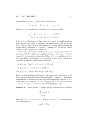
5.1 Basic Definitions
We have seen several examples of linear differential equations in the ex-
amples of the previous chapters. These include the spring mass system
(damped oscillator) and the operational amplifier in the presence of small
(non-saturating) input signals. More generally, many physical systems can
be modeled very accurately by linear differential equations. Electrical cir-
cuits are one example of a broad class of systems for which linear models can
be used effectively. Linear models are also broadly applicable in mechani-
143

156. 144 CHAPTER 5. LINEAR SYSTEMS
cal engineering, for example as models of small deviations from equilibria in
solid and fluid mechanics. Signal processing systems, including digital filters
of the sort used in CD and MP3 players, are another source of good exam-
ples, although often these are best modeled in discrete time (as described in
more detail in the exercises).
In many cases, we create systems with linear input/output response
through the use of feedback. Indeed, it was the desire for linear behav-
ior that led Harold S. Black, who invited the negative feedback amplifier,
to the principle of feedback as a mechanism for generating amplification.
Almost all modern single processing systems, whether analog or digital, use
feedback to produce linear or near-linear input/output characteristics. For
these systems, it is often useful to represent the input/output characteristics
as linear, ignoring the internal details required to get that linear response.
For other systems, nonlinearities cannot be ignored if one cares about
the global behavior of the system. The predator prey problem is one exam-
ple of this; to capture the oscillatory behavior of the coupled populations
we must include the nonlinear coupling terms. However, if we care about
what happens near an equilibrium point, it often suffices to approximate
the nonlinear dynamics by their local linearization, as we already explored
briefly in Section 4.3. The linearization is essentially an approximation of
the nonlinear dynamics around the desired operating point.
Linearity
We now proceed to define linearity of input/output systems more formally.
Consider a state space system of the form
dx
dt
= f(x, u)
y = h(x, u),
(5.1)
where x ∈ Rn, u ∈ Rp and y ∈ Rq. As in the previous chapters, we will
usually restrict ourselves to the single input, single output case by taking
p = q = 1. We also assume that all functions are smooth and that for a
reasonable class of inputs (e.g., piecewise continuous functions of time) that
the solutions of equation (5.1) exist for all time.
It will be convenient to assume that the origin x = 0, u = 0 is an
equilibrium point for this system ( ˙x = 0) and that h(0, 0) = 0. Indeed, we
can do so without loss of generality. To see this, suppose that (xe, ue) = (0, 0)
is an equilibrium point of the system with output ye = h(xe, ue) = 0. Then

157. 5.1. BASIC DEFINITIONS 145
we can define a new set of states, inputs, and outputs
˜x = x − xe ˜u = u − ue ˜y = y − ye
and rewrite the equations of motion in terms of these variables:
d
dt
˜x = f(˜x + xe, ˜u + ue) =: ˜f(˜x, ˜u)
˜y = h(˜x + xe, ˜u + ue) − ye =: ˜h(˜x, ˜u).
In the new set of variables, we have that the origin is an equilibrium point
with output 0, and hence we can carry our analysis out in this set of vari-
ables. Once we have obtained our answers in this new set of variables, we
simply have to remember to “translate” them back to the original coordi-
nates (through a simple set of additions).
Returning to the original equations (5.1), now assuming without loss of
generality that the origin is the equilibrium point of interest, we write the
output y(t) corresponding to initial condition x(0) = x0 and input u(t) as
y(t; x0, u). Using this notation, a system is said to be a linear input/output
system if the following conditions are satisfied:
(i) y(t; αx1 + βx2, 0) = αy(t; x1, 0) + βy(t; x2, 0)
(ii) y(t; αx0, δu) = αy(t; x0, 0) + δy(t; 0, u)
(iii) y(t; 0, δu1 + γu2) = δy(t; 0, u1) + γy(t; 0, u2).
Thus, we define a system to be linear if the outputs are jointly linear in the
initial condition response and the forced response. Property (ii) is the usual
decomposition of a system response into the homogeneous response (u = 0)
and the particular response (x0 = 0). Property (iii) is the formal definition
of the the principle of superposition illustrated in Figure 5.1.
Example 5.1 (Scalar system). Consider the first order differential equation
dx
dt
= ax + u
y = x
with x(0) = x0. Let u1 = A sin ω1t and u2 = B cos ω2t. The homogeneous
solution the ODE is
xh(t) = eat
x0

158. 146 CHAPTER 5. LINEAR SYSTEMS
time
u yLinear
System
y2
u1
+
u2
u1+u2
y1+y2
+
y1
time
Figure 5.1: Illustration of the principle of superposition. The output corresponding
to u1 + u2 is the sum of the outputs y1 and y2 due to the individual inputs.
and the two particular solutions are
x1(t) = −A
−ω1eat + ω1 cos ω1t + a sin ω1t
a2 + ω2
1
x2(t) = B
aeat − a cos ω2t + ω2 sin ω2t
a2 + ω2
2
.
Suppose that we now choose x(0) = αx0 and u = u1 +u2. Then the resulting
solution is
x(t) = eat
αx(0) +
Aω1
a2 + ω2
1
+
Ba
a2 + ω2
2
− A
ω1 cos ω1t + a sin ω1t
a2 + ω2
1
+ B
−a cos ω2t + ω2 sin ω2t
a2 + ω2
2
(5.2)
(to see this, substitute the equation in the differential equation). Thus, the
properties of a linear system are satisfied for this particular set of initial
conditions and inputs. ∇
We now consider a differential equation of the form
dx
dt
= Ax + Bu
y = Cx + Du,
(5.3)
where A ∈ Rn×n is a square matrix, B ∈ Rn is a column vector of length
n, C is a row vector of width n and D is a scalar. (In the case of a multi-
input systems, B, C and D becomes a matrices of appropriate dimension.)

159. 5.1. BASIC DEFINITIONS 147
Equation (5.3) is a system of linear, first order, differential equations with
input u, state x and output y. We now show that this system is a linear
input/output system, in the sense described above.
Proposition 5.1. The differential equation (5.3) is a linear input/output
system.
Proof. Let xh1(t) and xh2(t) be the solutions of the linear differential equa-
tion (5.3) with input u(t) = 0 and initial conditions x(0) = x01 and x02,
respectively, and let xp1(t) and xp2(t) be the solutions with initial condition
x(0) = 0 and inputs u1(t), u2(t) ∈ R. It can be verified by substitution that
the solution of equation (5.3) with initial condition x(0) = αx01 + βx02 and
input u(t) = δu1 + γu2 and is given by
x(t) = αxh1(t) + βxh2(t) + δxp1(t) + γxp2(t) .
The corresponding output is given by
y(t) = αyh1(t) + βyh2(t) + δyp1(t) + γyp2(t) .
By appropriate choices of α, β, δ and γ, properties (i)–(iii) can be verified.
As in the case of linear differential equations in a single variable, we
define the solution xh(t) with zero input as the homogeneous solution and
the solution xp(t) with zero initial condition as the particular solution. Fig-
ure 5.2 illustrates how these the homogeneous and particular solutions can
be superposed to form the complete solution.
It is also possible to show that if a system is input/output linear in the
sense we have described, that it can always be represented by a state space
equation of the form (5.3) through appropriate choice of state variables.
Time Invariance
Time invariance is another important concept that is can be used to describe
a system whose properties do not change with time. More precisely, if
the input u(t) gives output y(t), then if we shift the time at which the
input is applied by a constant amount a, u(t + a) gives the output y(t +
a). Systems that are linear and time-invariant, often called LTI systems,
have the interesting property that their response to an arbitrary input is
completely characterized by their response to step inputs or their response
to short “impulses”.

160. 148 CHAPTER 5. LINEAR SYSTEMS
0 20 40 60
−2
−1
0
1
2
Homogeneous
Input (u)
0 20 40 60
−2
−1
0
1
2
State (x
1
, x
2
)
0 20 40 60
−2
−1
0
1
2
Output (y)
0 20 40 60
−2
−1
0
1
2
Particular
0 20 40 60
−2
−1
0
1
2
0 20 40 60
−2
−1
0
1
2
0 20 40 60
−2
−1
0
1
2
Complete
time (sec)
0 20 40 60
−2
−1
0
1
2
time (sec)
0 20 40 60
−2
−1
0
1
2
time (sec)
Figure 5.2: Superposition of homogeeous and particular solutions. The first row
shows the input, state and output corresponding to the initial condition response.
The second row shows the same variables corresponding to zero initial condition,
but nonzero input. The third row is the complete solution, which is the sume of
the two individual solutions.
We will first compute the response to a piecewise constant input. Assume
that the sytem is initially at rest and consider the piecewise constant input
shown in Figure 5.3a. The input has jumps at times tk and its values after
the jumps are u(tk). The input can be viewed as a combination of steps:
the first step at time t0 has amplitude u(t0), the second step at time t1 has
amplitude u(t1) − u(t0), etc.
Assuming that the system is initially at an equilibrium point (so that
the initial condition response is zero), the response to the input can then be
obtained by superimposing the responses to a combination of step inputs.
Let H(t) be the response to a unit step applied at time t. The response
to the first step is then H(t − t0)u(t0), the response to the second step is

161. 5.2. THE CONVOLUTION EQUATION 149
0 2 4 6 8 10
0
0.2
0.4
0.6
0.8
1
Time (sec)
Input(u)
u(t
0
)
u(t
1
) u(t
1
) − u(t
0
)
(a)
0 2 4 6 8 10
−0.2
0
0.2
0.4
0.6
0.8
1
1.2
Time (sec)
Output(y)
(b)
Figure 5.3: Response to piecewise constant inputs: (a) a piecewise constant signal
can be represented as a sum of step signals; (b) the resulting output is the sum of
the individual outputs.
H(t − t1) u(t1) − u(t0) , and we find that the complete response is given by
y(t) = H(t − t0)u(t0) + H(t − t1) u(t1) − u(t0) + · · ·
= H(t) − H(t − t1) u(t0) + H(t − t1) − H(t − t2) u(t1)
=
∞
n=0
H(t − tn) − H(t − tn+1) u(tn)
=
∞
n=0
H(t − tn) − H(t − tn+1)
tn+1 − tn
tn+1 − tn u(tn).
An example of this computation is shown in Figure 5.3b.
The response to a continuous input signal is obtained by taking the limit
as tn+1 − tn → 0, which gives
y(t) =
∞
0
H′
(t − τ)u(τ)dτ, (5.4)
where H′ is the derivative of the step response, which is also called the im-
pulse response. The response of a linear time-invariant system to any input
can thus be computed from the step response. We will derive equation (5.4)
in a slightly different way in the next section.
5.2 The Convolution Equation
Equation (5.4) shows that the input response of a linear system can be
written as an integral over the inputs u(t). In this section we derive a more

162. 150 CHAPTER 5. LINEAR SYSTEMS
general version of this formula, which shows how to compute the output of
a linear system based on its state space representation.
The Matrix Exponential
Although we have shown that the solution of a linear set of differential equa-
tions defines a linear input/output system, we have not fully computed the
solution of the system. We begin by considering the homogeneous response
corresponding to the system
dx
dt
= Ax. (5.5)
For the scalar differential equation
˙x = ax x ∈ R, a ∈ R
the solution is given by the exponential
x(t) = eat
x(0).
We wish to generalize this to the vector case, where A becomes a matrix.
We define the matrix exponential as the infinite series
eX
= I + X +
1
2
X2
+
1
3!
X3
+ · · · =
∞
k=0
1
k!
Xk
, (5.6)
where X ∈ Rn×n is a square matrix and I is the n × n identity matrix. We
make use of the notation
X0
= I X2
= XX Xn
= Xn−1
X,
which defines what we mean by the “power” of a matrix. Equation (5.6) is
easy to remember since it is just the Taylor series for the scalar exponential,
applied to the matrix X. It can be shown that the series in equation (5.6)
converges for any matrix X ∈ Rn×n in the same way that the normal expo-
nential is defined for any scalar a ∈ R.
Replacing X in equation (5.6) by At where t ∈ R we find that
eAt
= I + At +
1
2
A2
t2
+
1
3!
A3
t3
+ · · · =
∞
k=0
1
k!
Ak
tk
,

163. 5.2. THE CONVOLUTION EQUATION 151
and differentiating this expression with respect to t gives
d
dt
eAt
= A + At +
1
2
A3
t2
+ · · · = A
∞
k=0
1
k!
Ak
tk
= AeAt
. (5.7)
Multiplying by x(0) from the right we find that x(t) = eAtx(0) is the solution
to the differential equation (5.5) with initial condition x(0). We summarize
this important result as a theorem.
Theorem 5.2. The solution to the homogeneous system of differential equa-
tion (5.5) is given by
x(t) = eAt
x(0).
Notice that the form of the solution is exactly the same as for scalar
equations.
The form of the solution immediately allows us to see that the solution
is linear in the initial condition. In particular, if xh1 is the solution to
equation (5.5) with initial condition x(0) = x01 and xh2 with initial condition
x02, then the solution with initial condition x(0) = αx01 + βx02 is given by
x(t) = eAt
αx01 + βx02 = αeAt
x01 + βeAt
x02) = αxh1(t) + βxh2(t).
Similarly, we see that the corresponding output is given by
y(t) = Cx(t) = αyh1(t) + βyh2(t),
where yh1 and yh2 are the outputs corresponding to xh1 and xh2.
We illustrate computation of the matrix exponential by three examples.
Example 5.2 (Double integrator). A very simple linear system that is useful
for understanding basic concepts is the second order system given by
¨q = u
y = q.
This system system is called a double integrator because the input u is
integrated twice to determine the output y.
In state space form, we write x = (q, ˙q) and
dx
dt
=


0 1
0 0

 x +


0
1

 u.

164. 152 CHAPTER 5. LINEAR SYSTEMS
The dynamics matrix of a double integrator is
A =


0 1
0 0


and we find by direct calculation that A2 = 0 and hence
eAt
=


1 t
0 1

 .
Thus the homogeneous solution (u = 0) for the double integrator is given
by
x(t) =


x1(0) + tx2(0)
x2(0)


y(t) = x1(0) + tx2(0).
∇
Example 5.3 (Undamped oscillator). A simple model for an oscillator, such
as the spring mass system with zero damping, is
m¨q + kq = u.
Putting the system into state space form, the dynamics matrix for this
system is
A =


0 1
− k
m 0


We have
eAt
=


cos ω0t 1
ω0
sin ω0t
−ω0 sin ω0t cos ω0t

 ω0 =
k
m
,
and the solution is then given by
x(t) = eAt
x(0) =


cos ω0t 1
ω0
sin ω0t
−ω0 sin ω0t cos ω0t




x1(0)
x2(0)

 .
This solution can be verified by differentiation:
d
dt
x(t) =


−ω0 sin ω0t cos ω0t
−ω2
0 cos ω0t −ω0 sin ω0t




x1(0)
x2(0)

 .
=


0 1
−ω2
0 0




cos ω0t 1
ω0
sin ω0t
−ω0 sin ω0t cos ω0t




x1(0)
x2(0)

 = Ax(t).

165. 5.2. THE CONVOLUTION EQUATION 153
If the damping c is nonzero, the solution is more complicated, but the matrix
exponential can be shown to be
eAt
= e
−ct
2m


eωdt + e−ωdt
2
+
eωdt − e−ωdt
2
√
c2 − 4km
eωdt − e−ωdt
√
c2 − 4km
−
keωdt − ke−ωdt
√
c2 − 4km
eωdt + e−ωdt
2
−
ceωdt − ce−ωdt
2
√
c2 − 4km
,


where ωd =
√
c2 − 4km/2m. Note that ωd can either be real or complex,
but in the case it is complex the combinations of terms will always yield a
positive value for the entry in the matrix exponential. ∇
Example 5.4 (Diagonal system). Consider a diagonal matrix
A =


λ1 0
λ2
...
0 λn


The kth power of At is also diagonal,
(At)k
=


λk
1tk 0
λk
2tk
...
0 λk
ntk


and it follows from the series expansion that the matrix exponential is given
by
eAt
=


eλ1t 0
eλ2t
...
0 eλnt


.
∇
Eigenvalues and Modes
The initial condition response of a linear system can be written in terms of a
matrix exponential involving the dynamics matrix A. The properties of the
matrix A therefore determine the resulting behavior of the system. Given a

166. 154 CHAPTER 5. LINEAR SYSTEMS
matrix A ∈ Rn×n, recall that λ is an eigenvalue of A with eigenvector v if λ
and v satisfy
Av = λv.
In general λ and v may be complex valued, although if A is real-valued then
for any eigenvalue λ, its complex conjugate λ∗ will also be an eigenvalue
(with v∗ as the corresponding eigenvector).
Suppose first that λ and v are a real-valued eigenvalue/eigenvector pair
for A. If we look at the solution of the differential equation for x(0) = v, it
follows from the definition of the matrix exponential that
eAt
v = I + At +
1
2
A2
t2
+ · · · v = (v + λtv +
λ2t2
2
v + · · · v = eλt
v.
The solution thus lies in the subspace spanned by the eigenvector. The
eigenvalue λ describes how the solution varies in time and is often called a
mode of the system. If we look at the individual elements of the vectors x
and v, it follows that
xi(t)
xj(t)
=
vi
vk
,
and hence the ratios of the components of the state x are constants. The
eigenvector thus gives the “shape” of the solution and is also called a mode
shape of the system.
Figure 5.4 illustrates the modes for a second order system. Notice that
the state variables have the same sign for the slow mode λ = −0.08 and
different signs for the fast mode λ = −0.62.
The situation is a little more complicated when the eigenvalues of A are
complex. Since A has real elements, the eigenvalues and the eigenvectors
are complex conjugates
λ = σ ± jω and v = u ± jw,
which implies that
u =
v + v∗
2
w =
v − v∗
2j
.
Making use of the matrix exponential, we have
eAt
v == eλt
(u + jw) = eσt
(u cos ωt − w sin ωt) + j(u sin ωt + w cos ωt) ,
which implies
eAt
u =
1
2
eAt
v + eAt
v∗
= ueσt
cos ωt − weσt
sin ωt
eAt
w =
1
2j
eAt
v − eAt
v∗
= ueσt
sin ωt + weσt
cos ωt.

167. 5.2. THE CONVOLUTION EQUATION 155
−1 −0.5 0 0.5 1
−1
−0.5
0
0.5
1
x
1
x2
(a)
0 10 20 30 40 50
0
0.5
1
0 10 20 30 40 50
0
0.5
1
x1,x2x1,x2
Slow mode λ = −0.08
Fast mode λ = −0.62
(b)
Figure 5.4: Illustration of the notion of modes for a second order system with real
eigenvalues. The left figure (a) shows the phase plane and the modes corresponds
to solutions that start on the eigenvectors. The time functions are shown in (b).
The ratios of the states are also computed to show that they are constant for the
modes.
A solution with initial conditions in the subspace spanned by the real part
u and imaginary part v of the eigenvector will thus remain in that subspace.
The solution will be logarithmic spiral characterized by σ and ω. We again
call λ a mode of the system and v the mode shape.
If a matrix A has a n distinct eigenvalues λ1, . . . , λn, then the initial con-
dition response can be written as a linear combination of the modes. To see
this, suppose for simplicity that we have all real eigenvalues with correspond-
ing unit eigenvectors v1, . . . , vn. From linear algebra, these eigenvectors are
linearly independent and we can write the initial condition x(0) as
x(0) = α1v1 + α2v2 + · · · αnvn.
Using linearity, the initial condition response can be written as
x(t) = α1eλ1t
v1 + α2eλ2t
v2 + · · · + αneλnt
vn.
Thus, the response is a linear combination the modes of the system, with
the amplitude of the individual modes growing or decaying as eλit. The case
for distinct complex eigenvalues follows similarly (the case for non-distinct
eigenvalues is more subtle and is described in the section on the Jordan
form, below).

168. 156 CHAPTER 5. LINEAR SYSTEMS
Linear Input/Output Response
We now return to the general input/output case in equation (5.3), repeated
here:
dx
dt
= Ax + Bu
y = Cx + Du.
(5.8)
Using the matrix exponential, the solution to equation (5.8) can be written
as follows.
Theorem 5.3. The solution to the linear differential equation (5.8) is given
by
x(t) = eAt
x(0) +
t
0
eA(t−τ)
Bu(τ)dτ. (5.9)
Proof. To prove this, we differentiate both sides and use the property (5.7)
of the matrix exponential. This gives
dx
dt
= AeAt
x(0) +
t
0
AeA(t−τ)
Bu(τ)dτ + Bu(t) = Ax + Bu,
which proves the result. Notice that the calculation is essentially the same
as for proving the result for a first order equation.
It follows from equations (5.8) and (5.9) that the input/output relation
for a linear system is given by
y(t) = CeAt
x(0) +
t
0
CeA(t−τ)
Bu(τ)dτ + Du(t). (5.10)
It is easy to see from this equation that the output is jointly linear in both
the initial conditions and the state: this follows from the linearity of ma-
trix/vector multiplication and integration.
Equation (5.10) is called the convolution equation and it represents the
general form of the solution of a system of coupled linear differential equa-
tions. We see immediately that the dynamics of the system, as characterized
by the matrix A, play a critical role in both the stability and performance
of the system. Indeed, the matrix exponential describes both what hap-
pens when we perturb the initial condition and how the system responds to
inputs.
Another interpretation of the convolution equation can be given using the

169. 5.2. THE CONVOLUTION EQUATION 157
0 20 40
0
0.2
0.4
0.6
0.8
1
1.2
u
t
(a)
0 10 20 30 40
0
0.2
0.4
0.6
0.8
1
y
t
(b)
Figure 5.5: (a) Pulses of width 5, 2 and 1, each with total area equal to 1. (b)
The pulse responses (solid) and impulse response (dashed) for a linear system with
eigenvalues λ = {−0.08, −0.62}.
concept of the impulse response of a system. Consider the application of an
input signal u(t) given by the following equation:
u(t) = pǫ(t) =



0 t < 0
1/ǫ 0 ≤ t < ǫ
0 t ≥ ǫ.
(5.11)
This signal is a “pulse” of duration ǫ and amplitude 1/ǫ, as illustrated in
Figure 5.5a. We define an impulse, δ(t), to be the limit of this signal as
ǫ → 0:
δ(t) = lim
ǫ→0
pǫ(t). (5.12)
This signal, sometimes called a delta function, is not physically achievable
but provides a convenient abstraction for understanding the response of
a system. Note that the integral of an impulse is a unit step function,
sometimes written as 1(t):
1(t) =
t
0
δ(τ) dτ =
t
0
lim
ǫ→0
pǫ(t) dτ t > 0
= lim
ǫ→0
t
0
pǫ(t) dτ = lim
ǫ→0
ǫ
0
1/ǫ dτ = 1 t > 0
In particular, the integral of an impulse over an arbitrarily short period of
time is identically 1.

170. 158 CHAPTER 5. LINEAR SYSTEMS
We define the impulse response of a system, h(t), to be the output cor-
responding to an impulse as its input:
h(t) =
t
0
CeA(t−τ)
Bδ(τ) dτ = CeAt
B, (5.13)
where the second equality follows from the fact that δ(t) is zero everywhere
except the origin and its integral is identically one. We can now write
the convolution equation in terms of the initial condition response and the
convolution of the impulse response and the input signal,
y(t) = CeAt
x(0) +
t
0
h(t − τ)u(τ) dτ. (5.14)
One interpretation of this equation, explored in Exercise 6, is that the re-
sponse of the linear system is the superposition of the response to an infinite
set of shifted impulses whose magnitude is given by the input, u(t). Note
that the second term in this equation is identical to equation (5.4) and it can
be shown that the impulse response is formally equivalent to the derivative
of the step response.
The use of pulses as an approximation of the impulse response provides a
mechanism for identifying the dynamics of a system from data. Figure 5.5b
shows the pulse responses of a system for different pulse widths. Notice that
the pulse responses approaches the impulse response as the pulse width goes
to zero. As a general rule, if the fastest eigenvalue of a stable system has
real part −λmax, then a pulse of length ǫ will provide a good estimate of
the impulse response if ǫλmax < 1. Note that for Figure 5.5, a pulse width
of ǫ = 1 s gives ǫλmax = 0.62 and the pulse response is very close to the
impulse response.
Coordinate Changes
The components of the input vector u and the output vector y are unique
physical signals, but the state variables depend on the coordinate system
chosen to represent the state. The choice of coordinates affects the values
of the matrices A, B and C that are used in the model. (The direct term D
is not affecting since it maps inputs to outputs.) We now investigate some
of the consequences of changing coordinate systems.
Introduce new coordinates z by the transformation z = Tx, where T is
an invertible matrix. It follows from equation (5.3) that
dz
dt
= T(Ax + Bu) = TAT−1
z + TBu = ˜Az + ˜Bu
y = Cx + DU = CT−1
z + Du = ˜Cz + Du.

171. 5.2. THE CONVOLUTION EQUATION 159
The transformed system has the same form as equation (5.3) but the ma-
trices A, B and C are different:
˜A = TAT−1
, ˜B = TB, ˜C = CT−1
, ˜D = D. (5.15)
As we shall see in several places later in the text, there are often special
choices of coordinate systems that allow us to see a particular property
of the system, hence coordinate transformations can be used to gain new
insight into the dynamics.
We can also compare the solution of the system in transformed coordi-
nates to that in the original state coordinates. We make use of an important
property of the exponential map,
eTST−1
= TeS
T−1
,
which can be verified by substitution in the definition of the exponential
map. Using this property, it is easy to show that
x(t) = T−1
z(t) = T−1
e
˜At
Tx(0) + T−1
t
0
e
˜A(t−τ) ˜Bu(τ) dτ.
From this form of the equation, we see that if it is possible to transform
A into a form ˜A for which the matrix exponential is easy to compute, we
can use that computation to solve the general convolution equation for the
untransformed state x by simple matrix multiplications. This technique is
illustrated in the next section.
Example 5.5 (Modal form). Suppose that A has n real, distinct eigenval-
ues, λ1, . . . , λn. It follows from matrix linear algebra that the corresponding
eigenvectors v1, . . . vn are linearly independent and form a basis for Rn. Sup-
pose that we transform coordinates according to the rule
x = Mz M =

v1 v2 · · · vn

 .
Setting T = M−1, it is easy to show that
˜A = TAT−1
= M−1
AM =


λ1 0
λ2
...
0 λn


.

172. 160 CHAPTER 5. LINEAR SYSTEMS
b
u(t) = sin ωt
m m
k
k
b
q1 q2
k
Figure 5.6: Coupled spring mass system.
To see this, note that if we multiple M−1AM by the basis elements
e1 =


1
0
0
...
0


e2 =


0
1
0
...
0


. . . en =


0
0
...
0
1


we get precisely λiei, which is the same as multiplying the diagonal form by
the canonical basis elements. Since this is true for each ei, i = 1, . . . , n and
since the these vectors form a basis for Rn, the transformed matrix must be
in the given form. This is precisely the diagonal form of Example 5.4, which
is also called the modal form for the system. ∇
Example 5.6 (Coupled mass spring system). Consider the coupled mass
spring system shown in Figure 5.6. The input to this system is the sinusoidal
motion of the end of rightmost spring and the output is the position of each
mass, q1 and q2. The equations of motion for the system are given by
m1 ¨q1 = −2kq1 − c ˙q1 + kq2
m2 ¨q2 = kq1 − 2kq2 − c ˙q2 + ku
In state-space form, we define the state to be x = (q1, q2, ˙q1, ˙q2) and we can
rewrite the equations as
˙x =


0 0 1 0
0 0 0 1
−2k
m
k
m − c
m 0
k
m −2k
m 0 − c
m


x +


0
0
0
k
m


u.
This is a coupled set of four differential equations and quite difficult to solve
in analytical form.

173. 5.3. STABILITY AND PERFORMANCE 161
We now define a transformation z = Tx that puts this system into a
simpler form. Let z1 = 1
2 (q1 + q2), z2 = ˙z1, z3 = 1
2 (q1 − q2) and z4 = ˙z3, so
that
z = Tx =
1
2


1 1 0 0
0 0 1 1
1 −1 0 0
0 0 1 −1


x.
Using the coordinate transformations described above (or simple substitu-
tion of variables, which is equivalent), we can write the system in the z
coordinates as
˙z =


0 1 0 0
− k
m − c
m 0 0
0 0 0 1
0 0 −3k
m − c
m


x +


0
k
2m
0
− k
2m


u.
Note that the resulting matrix equations are are block diagonal and hence
decoupled. We can thus solve for the solutions by computing the two sets of
second order system represented by the states (z1, z2) and (z3, z4). Indeed,
the functional form of each set of equations is identical to that of a single
spring mass system (Section 2.1).
Once we have solved the two sets of independent second order equations,
we can recover the dynamics in the original coordinates by inverting the state
transformation and writing x = T−1z. We can also determine the stability
of the system by looking at the stability of the independent second order
systems (Exercise 1). ∇
5.3 Stability and Performance
The special form of a linear system and its solution through the convolution
equation allow us to analytically solve for the stability of equilibrium points
and input/output performance properties.
Stability of Linear Systems
For a linear system, the stability of the equilibrium point at the origin can
be determined by looking at the eigenvalues of the stability matrix A:
λ(A) = {s ∈ C : det(sI − A) = 0}.
We use the notation λi for the ith eigenvalue of A, so that λi ∈ λ(A).

174. 162 CHAPTER 5. LINEAR SYSTEMS
The easiest class of linear systems to analyze are those whose system
matrices are in diagonal form. In this case, the dynamics have the form
dx
dt
=


λ1 0
λ2
...
0 λn


x +


β1
β2
...
βn


u
y =

γ1 γ2 · · · γn

 x + Du.
Using Example 5.4, it is easy to show that the state trajectories for this
system are independent of each other, so that we can write the solution in
terms of n individual systems
˙xi = λixi + βiu.
Each of these scalar solutions is of the form
xi(t) = eλit
x(0) +
t
0
eλ(t−τ)
u(t) dt.
If we consider the stability of the system when u = 0, we see that the
equilibrium point xe = 0 is stable if λi ≤ 0 and asymptotically stable if
λi < 0.
Very few systems are diagonal, but some systems can be transformed
into diagonal form via coordinate transformations. One such class of sys-
tems is those for which the dynamics matrix has distinct (non-repeating)
eigenvalues, as outlined in Example 5.5. In this case it is possible to find
a matrix T such that the matrix TAT−1 and the transformed system is in
diagonal form, with the diagonal elements equal to the the eigenvalues of the
original matrix A. We can reason about the stability of the original system
by noting that x(t) = T−1z(t) and so if the transformed system is stable (or
asymptotically stable) then the original system has the same type stability.
For more complicated systems, we make use of the following theorem,
proved in the next section:
Theorem 5.4. The system
˙x = Ax
is asymptotically stable if and only if all eigenvalues of A all have strictly
negative real part and is unstable if any eigenvalue of A has strictly positive
real part.

175. 5.3. STABILITY AND PERFORMANCE 163
v2
−
+
Rb
v1
v3
R1 Ra
R2
C2
C1
vo
Figure 5.7: Active filter circuit using an operational amplifier.
Example 5.7 (Active filter). Consider the op amp circuit shown in Fig-
ure 5.7. There are two energy storage elements, the capacitors C1 and C2.
We choose their voltages, v2 and v3, as states. The dynamics for the system
(Chapter 3, Exercise 5) are given by
˙x =


− 1
R1C1
− 1
RaC1
0
Rb
Ra
1
R2C2
− 1
R2C2

 x +


1
R1C1
0

 u
y =

0 1

 x,
where u = v1 and y = v3. The eigenvalues of the dynamics matrix, A, are
λ1 = −
1
R1C1
−
1
RaC1
λ2 = −
1
R2C2
.
Assuming all capacitances and resistances are positive, these eigenvalues
are both real and negative, and hence the equilibrium point at x = 0 is
asymptotically stable. This implies, in particular, that if no input voltage is
applied, the voltages around the system will all converge to zero as t → ∞.
∇
Jordan Form
Some matrices with equal eigenvalues cannot be transformed to diagonal
form. They can however be transformed to the Jordan form. In this form
the dynamics matrix has the eigenvalues along the diagonal. When there
are equal eigenvalues there may be ones appearing in the super diagonal
indicating that there is coupling between the states.
More specifically, we define a matrix to be in Jordan form if it can be

176. 164 CHAPTER 5. LINEAR SYSTEMS
written as
J =


J1 0 . . . 0
0 J2 0
0 . . .
... 0
0 . . . Jk


where Ji =


λi 1 0 . . . 0
0 λi 1 0
...
...
...
...
0 . . . 0 λi 1
0 . . . 0 0 λi


.
(5.16)
Each matrix Ji is called a Jordan block and λi for that block corresponds to
an eigenvalue of J.
Theorem 5.5 (Jordan decomposition). Any matrix A ∈ Rn×n can be trans-
formed into Jordan form with the eigenvalues of A determining λi in the
Jordan form.
Proof. See any standard text on linear algebra, such as Strang [Str88].
Converting a matrix into Jordan form can be very complicated, although
MATLAB can do this conversion for numerical matrices using the Jordan
function. The structure of the resulting Jordan form is particularly inter-
esting since there is no requirement that the individual λi’s be unique, and
hence for a given eigenvalue we can have one or more Jordan blocks of dif-
ferent size. We say that a Jordan block Ji is trivial if Ji is a scalar (1 × 1
block).
Once a matrix is in Jordan form, the exponential of the matrix can be
computed in terms of the Jordan blocks:
eJ
=


eJ1 0 . . . 0
0 eJ2 0
0 . . .
... 0
0 . . . eJk .


(5.17)
This follows from the block diagonal form of J. The exponentials of the
Jordan blocks can in turn be written as
eJit
=


eλit t eλit t2
2! eλit . . . tn−1
(n−1)! eλit
0 eλit t eλit . . . tn−2
(n−2)! eλit
eλit ...
... t eλit
0 eλit


(5.18)

177. 5.3. STABILITY AND PERFORMANCE 165
When there are multiple eigenvalues, the invariant subspaces represent-
ing the modes correspond to the Jordan blocks of the matrix A . Note that λ
may be complex, in which case the transformation T that converts a matrix
into Jordan form will also be complex. When λ has a non-zero imaginary
component, the solutions will have oscillatory components since
eσ+jωt
= eσt
(cos ωt + j sin ωt).
We can now use these results to prove Theorem 5.4.
Proof of Theorem 5.4. Let T ∈ Cn×n be an invertible matrix that trans-
forms A into Jordan form, J = TAT−1. Using coordinates z = Tx, we can
write the solution z(t) as
z(t) = eJt
z(0).
Since any solution x(t) can be written in terms of a solution z(t) with z(0) =
Tx(0), it follows that it is sufficient to prove the theorem in the transformed
coordinates.
The solution z(t) can be written as a combination of the elements of
the matrix exponential and from equation (5.18) these elements all decay
to zero for arbitrary z(0) if and only if Re λi < 0. Furthermore, if any λi
has positive real part, then there exists an initial condition z(0) such that
the corresponding solution increases without bound. Since we can scale this
initial condition to be arbitrarily small, it follows that the equilibrium point
is unstable if any eigenvalue has positive real part.
The existence of a canonical form allows us to prove many properties of
linear systems by changing to a set of coordinates in which the A matrix is
in Jordan form. We illustrate this in the following proposition, which follows
along the same lines as the proof of Theorem 5.4.
Proposition 5.6. Suppose that the system
˙x = Ax
has no eigenvalues with strictly positive real part and one or more eigenval-
ues with zero real part. Then the system is stable if and only if the Jordan
blocks corresponding to each eigenvalue with zero real part are scalar (1 × 1)
blocks.
Proof. Exercise 3.

178. 166 CHAPTER 5. LINEAR SYSTEMS
Input/Output Response
So far, this chapter has focused on the stability characteristics of a system.
While stability is often a desirably feature, stability alone may not be suf-
ficient in many applications. We will want to create feedback systems that
quickly react to changes and give high performance in measurable ways.
We return now to the case of an input/output state space system
dx
dt
= Ax + Bu
y = Cx + Du,
(5.19)
where x ∈ Rn is the state and u, y ∈ R are the input and output. The
general form of the solution to equation (5.19) is given by the convolution
equation:
y(t) = CeAt
x(0) +
t
0
CeA(t−τ)
Bu(τ)dτ + Du(t).
We see from the form of this equation that the solution consists of an initial
condition response and an input response.
The input response, corresponding to the second term in the equation
above, itself consists of two components—the transient response and steady
state response. The transient response occurs in the first period of time after
the input is applied and reflects the mismatch between the initial condition
and the steady state solution. The steady state response is the portion of
the output response that reflects the long term behavior of the system under
the given inputs. For inputs that are periodic, the steady state response will
often also be periodic. An example of the transient and steady state response
is shown in Figure 5.8.
Step Response
A particularly common form of input is a step input, which represents an
abrupt change in input from one value to another. A unit step is defined as
u = 1(t) =
0 t = 0
1 t > 0.
The step response of the system (5.3) is defined as the output y(t) starting
from zero initial condition (or the appropriate equilibrium point) and given
a step input. We note that the step input is discontinuous and hence is not

179. 5.3. STABILITY AND PERFORMANCE 167
0 10 20 30 40 50 60 70 80
−1
−0.5
0
0.5
1
input,u(t)
0 10 20 30 40 50 60 70 80
−0.1
−0.05
0
0.05
0.1
time (sec)
output,y(t)
Input
Output
Steady StateTransient
Figure 5.8: Transient versus steady state response. The top plot shows the input to
a linear system and the bottom plot the corresponding output. The output signal
initially undergoes a transient before settling into its steady state behavior.
physically implementable. However, it is a convenient abstraction that is
widely used in studying input/output systems.
We can compute the step response to a linear system using the convo-
lution equation. Setting x(0) = 0 and using the definition of the step input
above, we have
y(t) =
t
0
CeA(t−τ)
Bu(τ)dτ + Du(t)
=
t
0
CeA(t−τ)
Bdτ + D t > 0.
If A has eigenvalues with negative real part (implying that the origin is a
stable equilibrium point in the absence of any input), then we can rewrite
the solution as
y(t) = CA−1
eAt
B
transient
+ D − CA−1
B
steady state
t > 0. (5.20)

180. 168 CHAPTER 5. LINEAR SYSTEMS
0 5 10 15 20 25 30
0
0.5
1
1.5
2
time (sec)
Output
Rise time
Settling time
Overshoot
Steady state value
Figure 5.9: Sample step response
The first term is the transient response and decays to zero as t → ∞. The
second term is the steady state response and represents the value of the
output for large time.
A sample step response is shown in Figure 5.9. Several terms are used
when referring to a step response:
Steady state value The steady state value, yss, of a step response is the final
level of the output, assuming it converges.
Rise time The rise time, Tr, is the amount of time required for the signal to
go from 10% of its final value to 90% of its final value. It is possible
to define other limits as well, but in this book we shall use these
percentages unless otherwise indicated.
Overshoot The overshoot, Mp, is the percentage of the final value by which
the signal initially rises above the final value. This usually assumes
that future values of the signal do not overshoot the final value by
more than this initial transient, otherwise the term can be ambiguous.
Settling time The settling time, Ts, is the amount of time required for the
signal to stay within 5% of its final value for all future times. The
settling time is also sometimes defined as reaching 1% or 2% of the
final value (see Exercise 5).
In general these performance measures can depend on the amplitude of the
input step, but for linear systems it can be shown that the quantities defined
above are independent of the size of the step.

181. 5.3. STABILITY AND PERFORMANCE 169
Frequency Response
The frequency response of an input/output system measures the way in
which the system responds to a sinusoidal excitation on one of its inputs.
As we have already seen for linear systems, the particular solution associated
with a sinusoidal excitation is itself a sinusoid at the same frequency. Hence
we can compare the magnitude and phase of the output sinusoid to the
input. More generally, if a system has a sinusoidal output response at the
same frequency as the input forcing, we can speak of the frequency response
of the system.
To see this in more detail, we must evaluate the convolution equa-
tion (5.10) for u = cos ωt. This turns out to be a very messy computation,
but we can make use of the fact that the system is linear to simplify the
derivation. In particular, we note that
cos ωt =
1
2
ejωt
+ e−jωt
.
Since the system is linear, it suffices to compute the response of the system
to the complex input u(t) = est and we can always reconstruct the input to a
sinusoid by averaging the responses corresponding to s = jωt and s = −jωt.
Applying the convolution equation to the input u = est, we have
y(t) =
t
0
CeA(t−τ)
Besτ
dτ + Dest
=
t
0
CeA(t−τ)+sIτ
Bdτ + Dest
= eAt
t
0
Ce(sI−A)τ
Bdτ + Dest
.
If we assume that none of the eigenvalues of A are equal to s = ±jω, then
the matrix sI − A is invertible and we can write (after some algebra)
y(t) = CeAt
x(0) − (sI − A)−1
B
transient
+ D + C(sI − A)−1
B est
steady state
.
Notice that once again the solution consists of both a transient component
and a steady state component. The transient component decays to zero
if the system is asymptotically stable and the steady state component is
proportional to the (complex) input u = est.

182. 170 CHAPTER 5. LINEAR SYSTEMS
0 5 10 15 20 25 30
−1.5
−1
−0.5
0
0.5
1
1.5
time (sec)
Input,Output
A
u
A
y
∆T
T
input output
Figure 5.10: Frequency response, showing gain and phase. The phase lag is given
by θ = −2π∆T/T.
We can simplify the form of the solution slightly further by rewriting the
steady state response as
yss = Mejθ
est
= Me(st+jθ)
where
Mejθ
= C(sI − A)−1
B + D (5.21)
and M and θ represent the magnitude and phase of the complex number
D + C(sI − A)−1B. When s = jω, we say that M is the gain and θ is
the phase of the system at a given forcing frequency ω. Using linearity and
combining the solutions for s = +jω and s = −jω, we can show that if we
have an input u = Au sin(ωt + ψ) and output y = Ay sin(ωt + ϕ), then
gain(ω) =
Ay
Au
= M phase(ω) = ϕ − ψ = θ.
If the phase is positive, we say that the output “leads” the input, otherwise
we say it “lags” the input.
A sample frequency response is illustrated in Figure 5.10. The solid
line shows the input sinusoid, which has amplitude 1. The output sinusoid
is shown as a dashed line, and has a different amplitude plus a shifted
phase. The gain is the ratio of the amplitudes of the sinusoids, which can be
determined by measuring the height of the peaks. The phase is determined
by comparing the ratio of the time between zero crossings of the input and
output to the overall period of the sinusoid:
θ = −2π ó
δT
T
.

183. 5.3. STABILITY AND PERFORMANCE 171
10
−1
10
0
10
1
10
2
10
3
10
4
10
−6
10
−4
10
−2
10
0
10
2
Gain
10
−1
10
0
10
1
10
2
10
3
10
4
−150
−100
−50
0
Phase(deg)
Frequency (rad/sec)
Figure 5.11: Frequency response for the active filter from Example 5.7. The upper
plot shows the magnitude as a function of frequency (on a log-log scale) and the
lower plot shows the phase (on a log-linear scale).
Example 5.8 (Active filter). Consider the active filter presented in Ex-
ample 5.7. The frequency response for the system can be computed using
equation (5.21):
Mejθ
= C(sI − A)−1
B + D =
Rb/Ra
(1 + R2C2s)(R1+Ra
Ra
+ R1C1s)
s = jω.
The magnitude and phase are plotted in Figure 5.11 for Ra = 1kΩ, Rb =
100 kΩ, R1 = 100Ω, R2 = 5kΩ and C1 = C2 = 100 µF. ∇
The gain at frequency ω = 0 is called the zero frequency gain of the
system and corresponds to the ratio between a constant input and the steady
output:
M0 = CA−1
B + D.
Note that the zero frequency gain is only well defined if A is invertible (and,
in particular, if it does has not eigenvalues at 0). It is also important to note
that the zero frequency gain is only a relevant quantity when a system is

184. 172 CHAPTER 5. LINEAR SYSTEMS
stable about the corresponding equilibrium point. So, if we apply a constant
input u = r then the corresponding equilibrium point
xe = −A−1
Br
must be stable in order to talk about the zero frequency gain. (In electrical
engineering, the zero frequency gain is often called the “DC gain”. DC
stands for “direct current” and reflects the common separation of signals
in electrical engineering into a direct current (zero frequency) term and an
alternating current (AC) term.)
5.4 Second Order Systems
One class of systems that occurs frequently in the analysis and design of
feedback systems is second order, linear differential equations. Because of
their ubiquitous nature, it is useful to apply the concepts of this chapter to
that specific class of systems and build more intuition about the relationship
between stability and performance.
The canonical second order system is a differential equation of the form
¨q + 2ζω0 ˙q + ω2
0q = ku
y = q.
(5.22)
In state space form, this system can be represented as
˙x =


0 1
−ω2
0 −2ζω0

 x +


0
k

 u
y =

1 0

 x
(5.23)
The eigenvalues of this system are given by
λ = −ζω0 ± ω2
0(ζ2 − 1)
and we see that the origin is a stable equilibrium point if ω0 > 0 and
ζ > 0. Note that the eigenvalues are complex if ζ < 1 and real otherwise.
Equations (5.22) and (5.23) can be used to describe many second order
systems, including a damped spring mass system and an active filter, as
shown in the examples below.
The form of the solution depends on the value of ζ, which is referred to
as the damping factor for the system. If ζ > 1, we say that the system is

185. 5.4. SECOND ORDER SYSTEMS 173
overdamped and the natural response (u = 0) of the system is given by
y(t) =
βx10 + x20
β − α
e−αt
−
αx10 + x20
β − α
e−βt
where α = ω0(ζ + ζ2 − 1) and β = ω0(ζ − ζ2 − 1). We see that the
response consists of the sum of two exponentially decaying signals. If ζ = 1
then the system is critically damped and solution becomes
y(t) = e−ζω0t
x10 + (x20 + ζω0x10)t .
Note that this is still asymptotically stable as long as ω0 > 0, although the
second term in the solution is increasing with time (but more slowly than
the decaying exponential that multiplies it).
Finally, if 0 < ζ < 1, then the solution is oscillatory and equation (5.22)
is said to be underdamped. The parameter ω0 is referred to as the natural
frequency of the system, stemming from the fact that for small ζ, the eigen-
values of the system are approximately λ = −ζ ±jω0. The natural response
of the system is given by
y(t) = e−ζω0t
x10 cos ωdt +
ζω0
ωd
x10 +
1
ωd
x20 sin ωdt ,
where ωd = ω0 1 − ζ2. For ζ ≪ 1, ωd ≈ ω0 defines the oscillation frequency
of the solution and ζ gives the damping rate relative to ω0.
Because of the simple form of a second order system, it is possible to
solve for the step and frequency responses in analytical form. The solution
for the step response depends on the magnitude of ζ:
y(t) =
k
ω2
0
1 − e−ζω0t
cos ωdt +
ζ
1 − ζ2
e−ζω0t
sin ωdt ζ < 1
y(t) =
k
ω2
0
1 − e−ω0t
(1 + ω0t) ζ = 1
y(t) =
k
ω2
0
1 − e−ω0t
−
1
2(1 + ζ)
eω0(1−2ζ)t
ζ > 1,
(5.24)
where we have taken x(0) = 0. Note that for the lightly damped case
(ζ < 1) we have an oscillatory solution at frequency ωd, sometimes called
the damped frequency.
The step responses of systems with k = ω2 and different values of ζ are
shown in Figure 5.12, using a scaled time axis to allow an easier comparison.

186. 174 CHAPTER 5. LINEAR SYSTEMS
0 5 10 15
0
0.5
1
1.5
2
ω0t
y
ζ
Figure 5.12: Normalized step responses h for the system (5.23) for ζ = 0 (dashed),
0.1, 0.2, 0.5, 0.707 (dash dotted), 1, 2, 5 and 10 (dotted).
The shape of the response is determined by ζ and the speed of the response
is determined by ω0 (including in the time axis scaling): the response is
faster if ω0 is larger. The step responses have an overshoot of
Mp =
e−πζ/
√
1−ζ2
for |ζ| < 1
0 for ζ ≥ 1.
(5.25)
For ζ < 1 the maximum overshoot occurs at
tmax =
π
ω0 1 − ζ2
. (5.26)
The maximum decreases and is shifted to the right when ζ increases and it
becomes infinite for ζ = 1, when the overshoot disappears.
The frequency response can also be computed explicitly and is given by
Mejθ
=
ω2
0
(jω)2 + 2ζω0(jω) + ω2
0
=
ω2
0
ω2
0 − ω2 + 2jζω0ω
.
A graphical illustration of the frequency response is given in Figure 5.13.
Notice the resonance peak that increases with decreasing ζ. The peak is
often characterized by is Q-value, defined as Q = 1/2ζ.
Example 5.9 (Damped spring mass). The dynamics for a damped spring
mass system are given by
m¨q + c ˙q + kq = u,
where m is the mass, q is the displacement of the mass, c is the coefficient
of viscous friction, k is the spring constant and u is the applied force. We

187. 5.4. SECOND ORDER SYSTEMS 175
10
−1
10
0
10
1
10
−2
10
−1
10
0
10
1
10
−1
10
0
10
1
−150
−100
−50
0
ζ
ζ
Figure 5.13: Frequency response of a the second order system (5.23). The upper
curve shows the gain ratio, M, and the lower curve shows the phase shift, θ. The
parameters is Bode plot of the system with ζ = 0 (dashed), 0.1, 0.2, 0.5, 0.7 and
1.0 (dashed-dot).
can convert this into the standard second order for by dividing through by
m, giving
¨q +
c
m
˙q +
k
m
q =
1
m
u.
Thus we see that the spring mass system has natural frequency and damping
ratio given by
ω0 =
k
m
ζ =
c
2
√
km
(note that we have use the symbol k for the stiffness here; it should not be
confused with the gain term in equation (5.22)). ∇
One of the other reasons why second order systems play such an important
role in feedback systems is that even for more complicated systems the
response is often dominated by the “dominant eigenvalues”. To define these
more precisely, consider a system with eigenvalues λi, i = 1, . . . , n. We

188. 176 CHAPTER 5. LINEAR SYSTEMS
define the damping factor for a complex eigenvalue λ to be
ζ =
−Re λ
|λ|
We say that a complex conjugate pair of eigenvalues λ, λ∗ is a dominant
pair if it has the lowest damping factor compared with all other eigenvalues
of the system.
Assuming that a system is stable, the dominant pair of eigenvalues tends
to be the most important element of the response. To see this, assume that
we have a system in Jordan form with a simple Jordan block corresponding
to the dominant pair of eigenvalues:
˙z =


λ
λ∗
J2
...
Jk


z + Bu
y = Cz.
(Note that the state z may be complex due to the Jordan transformation.)
The response of the system will be a linear combination of the responses
from each of the individual Jordan subsystems. As we see from Figure 5.12,
for ζ < 1 the subsystem with the slowest response is precisely the one with
the smallest damping factor. Hence when we add the responses from each
of the individual subsystems, it is the dominant pair of eigenvalues that will
be dominant factor after the initial transients due to the other terms in the
solution. While this simple analysis does not always hold (for example, if
some non-dominant terms have large coefficients due to the particular form
of the system), it is often the case that the dominant eigenvalues dominate
the (step) response of the system. The following example illustrates the
concept.
5.5 Linearization
As described in the beginning of the chapter, a common source of linear
system models is through the approximation of a nonlinear system by a linear
one. These approximations are aimed at studying the local behavior of a
system, where the nonlinear effects are expected to be small. In this section
we discuss how to locally approximate a system by its linearization and what

189. 5.5. LINEARIZATION 177
can be said about the approximation in terms of stability. We begin with
an illustration of the basic concept using the speed control example from
Chapter 2.
Example 5.10 (Cruise control). The dynamics for the cruise control system
are derived in Section 3.1 and have the form
m
dv
dt
= αnuT(αnv) − mgCr − 1
2ρCvAv2
− mg sin θ, (5.27)
where the first term on the right hand side of the equation is the force gen-
erated by the engine and the remaining three terms are the rolling friction,
aerodynamic drag and gravitational disturbance force. There is an equilib-
rium (ve, ue) when the force applied by the engine balances the disturbance
forces.
To explore the behavior of the system near the equilibrium we will lin-
earize the system. A Taylor series expansion of equation (5.27) around the
equilibrium gives
d(v − ve)
dt
= a(v − ve) − bg(θ − θe) + b(u − ue) (5.28)
where
a =
ueα2
nT′(αnve) − ρCvAve
m
bg = g cos θe b =
αnT(αnve)
m
(5.29)
and terms of second and higher order have been neglected. For a car in
fourth gear with ve = 25 m/s, θe = 0 and the numerical values for the car
from Section 3.1, the equilibrium value for the throttle is ue = 0.1687 and
the model becomes
d(v − ve)
dt
= −0.0101(v − ve) + 1.3203(u − ue) − 9.8(θ − θe) (5.30)
This linear model describes how small perturbations in the velocity about
the nominal speed evolve in time.
Figure 5.14, which shows a simulation of a cruise controller with linear
and nonlinear models, indicates that the differences between the linear and
nonlinear models is not visible in the graph. ∇
Linear Approximation
To proceed more formally, consider a single input, single output nonlinear
system
dx
dt
= f(x, u) x ∈ Rn
, u ∈ R
y = h(x, u) y ∈ R
(5.31)

190. 178 CHAPTER 5. LINEAR SYSTEMS
0 5 10 15 20 25 30
19
19.5
20
20.5
0 5 10 15 20 25 30
0
0.5
1
ThrottleVelocity[m/s]
Time [s]
Figure 5.14: Simulated response of a vehicle with PI cruise control as it climbs a
hill with a slope of 4◦
. The full lines is the simulation based on a nonlinear model
and the dashed line shows the corresponding simulation using a linear model. The
controller gains are kp = 0.5 and ki = 0.1.
with an equilibrium point at x = xe, u = ue. Without loss of generality,
we assume that xe = 0 and ue = 0, although initially we will consider the
general case to make the shift of coordinates explicit.
In order to study the local behavior of the system around the equilib-
rium point (xe, ue), we suppose that x − xe and u − ue are both small, so
that nonlinear perturbations around this equilibrium point can be ignored
compared with the (lower order) linear terms. This is roughly the same type
of argument that is used when we do small angle approximations, replacing
sin θ with θ and cos θ with 1 for θ near zero.
In order to formalize this idea, we define a new set of state variables z,
inputs v, and outputs w:
z = x − xe v = u − ue w = y − h(xe, ue).
These variables are all close to zero when we are near the equilibrium point,
and so in these variables the nonlinear terms can be thought of as the higher
order terms in a Taylor series expansion of the relevant vector fields (assum-
ing for now that these exist).
Example 5.11. Consider a simple scalar system,
˙x = 1 − x3
+ u.

191. 5.5. LINEARIZATION 179
The point (xe, ue) = (1, 0) is an equilibrium point for this system and we
can thus set
z = x − 1 v = u.
We can now compute the equations in these new coordinates as
˙z =
d
dt
(x − 1) = ˙x
= 1 − x3
+ u = 1 − (z + 1)3
+ v
= 1 − z3
− 3z2
− 3z − 1 + v = −3z − 3z2
− z3
+ v.
If we now assume that x stays very close to the equilibrium point, then
z = x − xe is small and z ≪ z2 ≪ z3. We can thus approximate our system
by a new system
˙z = −3z + v.
This set of equations should give behavior that is close to that of the original
system as long as z remains small. ∇
More formally, we define the Jacobian linearization of the nonlinear sys-
tem (5.31) as
˙z = Az + Bv
w = Cz + Dv,
(5.32)
where
A =
∂f(x, u)
∂x (xe,ue)
B =
∂f(x, u)
∂u (xe,ue)
C =
∂h(x, u)
∂x (xe,ue)
D =
∂h(x, u)
∂u (xe,ue)
(5.33)
The system (5.32) approximates the original system (5.31) when we are near
the equilibrium point that the system was linearized about.
It is important to note that we can only define the linearization of a sys-
tem about an equilibrium point. To see this, consider a polynomial system
˙x = a0 + a1x + a2x2
+ a3x3
+ u,
where a1 = 0. There are a family of equilibrium points for this system given
by (xe, ue) = (xe, −a0 −a1xe −a2x2
e −a3x3
e) and we can linearize around any
of these. Suppose that we try to linearize around the origin of the system,
x = 0, u = 0. If we drop the higher order terms in x, then we get
˙x = a0 + a1x + u,

192. 180 CHAPTER 5. LINEAR SYSTEMS
which is not the Jacobian linearization if a0 = 0. The constant term must
be kept and this is not present in (5.32). Furthermore, even if we kept the
constant term in the approximate model, the system would quickly move
away from this point (since it is “driven” by the constant term a0) and
hence the approximation could soon fail to hold.
Software for modeling and simulation frequently has facilities for per-
forming linearization symbolically or numerically. The MATLAB command
trim finds the equilibrium and linmod extracts linear state-space models
from a SIMULINK system around an operating point.
Example 5.12 (Vehicle steering). Consider the vehicle steering system in-
troduced in Section 2.8. The nonlinear equations of motion for the system
are given by equations (2.21)–(2.23) and can be written as
d
dt


x
y
θ


=


v0
cos (α+θ)
cos α
v0
sin (α+θ)
cos α
v0
b tan δ


,
where x, y and θ are the position and orientation of the center of mass of
the vehicle, v0 is the velocity of the rear wheel, δ is the angle of the front
wheel and α is the anglular devitation of the center of mass from the rear
wheel along the instantaneous circle of curvature determined by the front
wheel:
α(δ) = arctan
a tan δ
b
.
We are interested in the motion of the vehicle about a straight line path
(θ = θ0) with fixed velocity v0 = 0. To find the relevant equilibrium point,
we first set ˙θ = 0 and we see that we must have δ = 0, corresponding to the
steering wheel being straight. This also yields α = 0. Looking at the first
two equations in the dynamics, we see that the motion in the xy direction
is by definition not at equilibrium since ˙x2 + ˙y2 = v2
0 = 0. Therefore we
cannot formally linearize the full model.
Suppose instead that we are concerned with the lateral deviation of the
vehicle from a straight line. For simplicity, we let θ0 = 0, which corresponds
to driving along the x axis. We can then focus on the equations of motion
in the y and θ directions, for which we have
d
dt


y
θ

 =


v0
sin (α+θ)
cos α
v0
b tan δ

 .

193. 5.5. LINEARIZATION 181
Abusing notation, we write x = (y, θ) and u = δ so that
f(x, u) =


v0
sin(α(u)+x2)
cos α(u)
v0
b tan u,


where the equilibrium point of interest is now given by x = (0, 0) and u = 0.
To compute the linearization the model around the equilibrium point,
we make use of the formulas (5.33). A straightforward calculation yields
A =
∂f(x, u)
∂x x=0
u=0
=


0 v0
0 0

 δ B =
∂f(x, u)
∂u x=0
u=0
=


v0
a
b
v0
b


and the linearized system
˙z = Az + Bv (5.34)
thus provides an approximation to the original nonlinear dynamics.
A model can often be simplified further by introducing normalized di-
mension free variables. For this system, we can normalize lengths by the
wheel base b and introduce a new time variable τ = v0t/b. The time unit is
thus the time is takes for the vehicle to travel one wheel base. We similarly
normalize the lateral position and write w1 = y/b, w2 = θ. The model (5.34)
then becomes
dw
dτ
=


w2 + αv
v

 =


0 1
0 0

 w +


α
1

 v
y =

1 0

 w
(5.35)
The normalized linear model for vehicle steering with non-slipping wheels is
thus a linear system with only one parameter α = a/b. ∇
Feedback Linearization
Another type of linearization is the use of feedback to convert the dynamics
of a nonlinear system into a linear one. We illustrate the basic idea with an
example.
Example 5.13 (Cruise control). Consider again the cruise control system
from Example 5.10, whose dynamics is given in equation (5.27). If we choose
u as a feedback law of the form
u =
1
αnT(αnv)
u′
+ mgCr +
1
2
ρCvAv2
(5.36)

194. 182 CHAPTER 5. LINEAR SYSTEMS
then the resulting dynamics become
m
dv
dt
= u′
+ d (5.37)
where d = mg sin θ is the disturbance force due the slope of the road. If
we now define a feedback law for u′ (such as a PID controller), we can use
equation (5.36) to compute the final input that should be commanded.
Equation (5.37) is a linear differential equation. We have essentially
“inverted out” the nonlinearity through the use of the feedback law (5.36).
This requires that we have an accurate measurement of the vehicle velocity
v as well as an accurate model of the torque characteristics of the engine,
gear ratios, drag and friction characteristics and mass of the car. While such
a model is not generally available (remembering that the parameter values
can change), if we design a good feedback law for u′, then we can achieve
robustness to these uncertainties. ∇
More generally, we say that a system of the form
dx
dt
= f(x, u)
y = h(x)
is feedback linearizable if we can find a control law u = α(x, v) such that
the resulting closed loop system is input/output linear with input v and
output u. To fully characterize such systems is beyond the scope of this
text, but we note that in addition to changes in the input, we must also
allow for (nonlinear) changes in the states that are used to describe the
system, keeping only the input and output variables fixed. More details
of this process can be found in the the textbooks by Isidori [Isi89] and
Khalil [Kha92].
One case the comes up relatively frequently, and is hence worth special
mention, is the set of mechanical systems of the form
M(q)¨q + C(q, ˙q) ˙q + N(q, ˙q) = B(q)u.
Here q ∈ Rn is the configuration of the mechanical system, M(q) ∈ Rn×n
is the configuration-dependent inertia matrix, C(q, ˙q) ˙q ∈ Rn represents the
Coriolis forces, N(q, ˙q) ∈ Rn are additional nonlinear forces (such as stiffness
and friction) and B(q) ∈ Rn×p is the input matrix. If p = n then we have
the same number of inputs and configuration variables and if we further

195. 5.6. FURTHER READING 183
have that B(q) is an invertible matrix for all configurations q, then we can
choose
u = B−1
(q) (M(q)v − C(q, ˙q) ˙q − N(q, ˙q)) . (5.38)
The resulting dynamics become
M(q)¨q = M(q)v =⇒ ¨q = v,
which is a linear system. We can now use the tools of linear systems theory
to analyze and design control laws for the linearized system, remembering
to apply equation (5.38) to obtain the actual input that will be applied to
the system.
This type of control is common in robotics, where it goes by the name
of computed torque, and aircraft flight control, where it is called dynamic
inversion.
Local Stability of Nonlinear Systems
Having constructed a linearized model around an equilibrium point, we can
now ask to what extent this model predicts the behavior of the original
nonlinear system. The following theorem gives a partial answer for the case
of stability.
Theorem 5.7. Consider the system (5.31) and let A ∈ Rn×n be defined as
in equations (5.32) and (5.33). If the real part of the eigenvalues of A are
strictly less than zero, then xe is a locally asymptotically stable equilibrium
point of (5.31).
This theorem shows that global asymptotic stability of the linearization
implies local asymptotic stability of the original nonlinear system. The esti-
mates provided by the proof of the theorem can be used to give a (conserva-
tive) bound on the domain of attraction of the origin. Systematic techniques
for estimating the bounds on the regions of attraction of equilibrium points
of nonlinear systems is an important area of research and involves searching
for the “best” Lyapunov functions.
The proof of this theorem is the beyond the scope of this text, but can
be found in [Kha92].
5.6 Further Reading
The idea to characterize dynamics by considering the responses to step in-
puts is due to Heaviside. The unit step is therefore also called the Heaviside

196. 184 CHAPTER 5. LINEAR SYSTEMS
step function. The majority of the material in this chapter is very classical
and can be found in most books on dynamics and control theory, includ-
ing early works on control such as James, Nichols and Phillips [JNP47], and
more recent textbooks such as Franklin, Powell and Emami-Naeni [FPEN05]
and Ogata [Oga01]. The material on feedback linearization is typically pre-
sented in books on nonlinear control theory, such as Khalil [Kha92]. Tracer
methods are described in [She62].
5.7 Exercises
1. Compute the full solution to the couple spring mass system in Ex-
ample 5.6 by transforming the solution for the block diagonal system
back into the original set of coordinates. Show that the system is
asymptotically stable if m, b and k are all greater than zero.
2. Using the computation for the matrix exponential, show that equa-
tion (5.18) holds for the case of a 3×3 Jordan block. (Hint: decompose
the matrix into the form S + N where S is a diagonal matrix.)
3. Prove Proposition 5.6.
4. Show that the step response for an asymptotically stable linear system
is given by equation (5.20).
5. Consider a first order system of the form
˙x = −τx + u
y = x.
We say that the parameter τ is the time constant for the system since
the zero input system approaches the origin as eτt. For a first order
system of this form, show that the rise time of the system is approxi-
mately 2τ, a 5% settling time corresponds to approximately 3τ and a
2% settling time corresponds to approximately 4τ.
6. Show that a signal u(t) can be decomposed in terms of the impulse
function δ(t) as
u(t) =
t
0
δ(t − τ)u(τ) dτ
and use this decomposition plus the principle of superposition to show
that the response of a linear system to an input u(t) (assuming zero

197. 5.7. EXERCISES 185
initial condition) can be written as
y(t) =
t
0
h(t − τ)u(τ) dτ,
where h(t) is the impulse response of the system.
7. Consider a linear discrete time system of the form
xk+1 = Axk + Buk
yk = Cxk + Duk.
(a) Show that the general form of the output of a discrete time linear
system is given by the discrete time convolution equation:
yk = CAk
x0 +
k
i=0
CAi
Bui + Duk
(b) Show that a discrete time linear system is asymptotically stable if
and only if all eigenvalues of A have magnitude strictly less than
1.
(c) Let uk = A sin(ωk) represent an oscillatory input with frequency
ω < π (to avoid “aliasing”). Show that the steady state compo-
nent of the response has gain M and phase θ where
Mejθ
= C(jωI − A)−1
B + D.
(d) Show that if we have a nonlinear discrete time system
xk = f(xk, uk) xk ∈ Rn
, u ∈ R
yk = h(xk, u)k) y ∈ R
then we can linearize the system around an equilibrium point
(xe, ue) by defining the matrices A, B, C and D as in equa-
tion (5.33).
8. Consider the consensus protocol introduced in Example 2.13. Show
that if the connectivity graph of the sensor network is connected, then
we can find a gain γ such that the agent states converge to the average
value of the measure quantity.

198. 186 CHAPTER 5. LINEAR SYSTEMS

199. Chapter 6
State Feedback
Intuitively, the state may be regarded as a kind of information storage or
memory or accumulation of past causes. We must, of course, demand that
the set of internal states Σ be sufficiently rich to carry all information about
the past history of Σ to predict the effect of the past upon the future. We do
not insist, however, that the state is the least such information although this
is often a convenient assumption.
R. E. Kalman, P. L. Falb and M. A. Arbib, 1969 [KFA69].
This chapter describes how feedback of a system’s state can be used
shape the local behavior of a system. The concept of reachability is intro-
duced and used to investigate how to “design” the dynamics of a system
through assignment of its eigenvalues. In particular, it will be shown that
under certain conditions it is possible to assign the system eigenvalues to
arbitrary values by appropriate feedback of the system state.
6.1 Reachability
One of the fundamental properties of a control system is what set of points in
the state space can be reached through the choice of a control input. It turns
out that the property of “reachability” is also fundamental in understanding
the extent to which feedback can be used to design the dynamics of a system.
Definition
We begin by disregarding the output measurements of the system and fo-
cusing on the evolution of the state, given by
dx
dt
= Ax + Bu, (6.1)
187

200. 188 CHAPTER 6. STATE FEEDBACK
x0
x(T)
R(x0, ≤ T)
(a) (b)
Figure 6.1: The reachable set for a control system: (a) the set R(x0, ≤ T) is the set
of points reachable from x0 in time less than T; (b) phase portrait for the double
integrator showing the natural dynamics (horizontal arrows), the control inputs
(vertical arrows) and a sample path to the origin.
where x ∈ Rn, u ∈ R, A is an n × n matrix and B an n × 1 matrix. A
fundamental question is whether it is possible to find control signals so that
any point in the state space can be reached through some choice of input.
To study this, we define the reachable set R(x0, ≤ T) as the set of all points
xf such that there exists an input u(t), 0 ≤ t ≤ T that steers the system
from x(0) = x0 to x(T) = xf , as illustrated in Figure 6.1.
Definition 6.1 (Reachability). A linear system is reachable if for any x0, xf ∈
Rn there exists a T > 0 and u: [0, T] → R such that the corresponding so-
lution satisfies x(0) = x0 and x(T) = xf .
The set of points that we are most interested in reaching is the set of
equilibrium points of the system (since we can remain at those points once
we get there). The set of all possible equilibria for constant controls is given
by
E = {xe : Axe + bue = 0 for some ue ∈ R}.
This means that possible equilibria lie in a one (or possibly higher) dimen-
sional subspace. If the matrix A is invertible this subspace is spanned by
A−1B.
In addition to reachability of equilibrium points, we can also ask whether
it is possible to reach all points in the state space in a transient fashion. The
following example provides some insight into the possibilities.
Example 6.1 (Double integrator). Consider a linear system consisting of
a double integrator, whose dynamics are given by
˙x1 = x2
˙x2 = u.

201. 6.1. REACHABILITY 189
Figure 6.1b shows a phase portrait of the system. The open loop dynamics
(u = 0) are shown as horizontal arrows pointed to the right for x2 > 0 and
the the left for x2 < 0. The control input is represented by a double arrow
in the vertical direction, corresponding to our ability to set the value of ˙x2.
The set of equilibrium points E corresponds to the x1 axis, with ue = 0.
Suppose first that we wish to reach the origin from an initial condition
(a, 0). We can directly move the state up and down in the phase plane, but
we must rely on the natural dynamics to control the motion to the left and
right. If a > 0, we can move the origin by first setting u < 0, which will case
x2 to become negative. Once x2 < 0, the value of x1 will begin to decrease
and we will move to the left. After a while, we can set u2 to be positive,
moving x2 back toward zero and slowing the motion in the x1 direction. If
we bring x2 > 0, we can move the system state in the opposite direction.
Figure 6.1b shows a sample trajectory bringing the system to the origin.
Note that if we steer the system to an equilibrium point, it is possible to
remain there indefinitely (since ˙x1 = 0 when x2 = 0), but if we go to any
other point in the state space, we can only pass through the point in a
transient fashion. ∇
To find general conditions under which a linear system is reachable, we
will first give a heuristic argument based on formal calculations with impulse
functions. We note that if we can reach all points in the state space through
some choice of input, then we can also reach all equilibrium points. Hence
reachability of the entire state space implies reachability of all equilibrium
points.
Testing for Reachability
When the initial state is zero, the response of the state to a unit step in the
input is given by
x(t) =
t
0
eA(t−τ)
Bdτ = A−1
(eAt
− I)B (6.2)
The derivative of a unit step function is the impulse function, δ(t), defined in
Section 5.2. Since derivatives are linear operations, it follows (see Exercise 7)
that the response of the system to an impulse function is thus the derivative
of equation (6.2) (i.e., the impulse response),
dx
dt
= eAt
B.

202. 190 CHAPTER 6. STATE FEEDBACK
Similarly we find that the response to the derivative of a impulse function
is
d2x
dt2
= AeAt
B.
Continuing this process and using the linearity of the system, the input
u(t) = α1δ(t) + α2
˙δ(t) + α¨δ(t) + · · · + αnδ(n−1)
(t)
gives the state
x(t) = α1eAt
B + α2AeAt
B + α3A2
eAt
B + · · · + αnAn−1
eAt
B.
Hence, right after the initial time t = 0, denoted t = 0+, we have
x(0+) = α1B + α2AB + α3A2
B + · · · + αnAn−1
B.
The right hand is a linear combination of the columns of the matrix
Wr =

B AB · · · An−1B

 . (6.3)
To reach an arbitrary point in the state space we thus require that there are
n linear independent columns of the matrix Wr. The matrix is called the
reachability matrix.
An input consisting of a sum of impulse functions and their derivatives
is a very violent signal. To see that an arbitrary point can be reached with
smoother signals we can also argue as follows. Assuming that the initial
condition is zero, the state of a linear system is given by
x(t) =
t
0
eA(t−τ)
Bu(τ)dτ =
t
0
eAτ
Bu(t − τ)dτ.
It follows from the theory of matrix functions, specifically the Cayley-Hamilton
theorem [Str88] that
eAτ
= Iα0(τ) + Aα1(τ) + · · · + An−1
αn−1(τ),
where αi(τ) are scalar functions, and we find that
x(t) = B
t
0
α0(τ)u(t − τ) dτ + AB
t
0
α1(τ)u(t − τ) dτ+
· · · + An−1
B
t
0
αn−1(τ)u(t − τ) dτ.
Again we observe that the right hand side is a linear combination of the
columns of the reachability matrix Wr given by equation (6.3). This basic
approach leads to the following theorem.

203. 6.1. REACHABILITY 191
l
M
F
p
θ
m
(a) (b)
Figure 6.2: Balance system: (a) Segway human transportation system and (b)
simplified diagram.
Theorem 6.1. A linear system is reachable if and only the reachability
matrix Wr is invertible.
The formal proof of this theorem is beyond the scope of this text, but
follows along the lines of the sketch above and can be found in most books
on linear control theory, such as [CD91]. We illustrate the concept of reach-
ability with the following example.
Example 6.2 (Reachability of balance systems). Consider the balance sys-
tem introduced in Example 2.1 and shown in Figure 6.2. Recall that this
system is a model for a class of examples in which the center of mass is
balanced above a pivot point. One example is the Segway transportation
system shown in the left hand figure, in which a natural question to ask is
whether we can move from one stationary point to another by appropriate
application of forces through the wheels.
The nonlinear equations of motion for the system are given in equa-
tion (2.7) and repeated here:
(M + m)¨p − ml cos θ ¨θ = −c ˙p + ml sin θ ˙θ2
+ F
(J + ml2
)¨θ − ml cos θ ¨p = −γ ˙+θmgl sin θ,
(6.4)
For simplicity, we take c = γ = 0. Linearizing around the equilibrium point

204. 192 CHAPTER 6. STATE FEEDBACK
S
S
Figure 6.3: A non-reachable system.
xe = (p, 0, 0, 0), the dynamics matrix and the control matrix are
A =


0 0 1 0
0 0 0 1
0 m2l2g
MtJt−m2l2 0 0
0 Mtmgl
MtJt−m2l2 0 0


B =


0
0
Jt
MtJt−m2l2
lm
MtJt−m2l2


,
The reachability matrix is
Wr =


0 Jt
MtJt−m2l2 0 gl3m3
(MtJt−m2l2)2
0 lm
MtJt−m2l2 0 gl2m2(m+M)
(MtJt−m2l2)2
Jt
MtJt−m2l2 0 gl3m3
(MtJt−m2l2)2 0
lm
MtJt−m2l2 0 g2l2m2(m+M)
(MtJt−m2l2)2 0


. (6.5)
This matrix has determinant
det(Wr) =
g2l4m4
(MtJt − m2l2)4
= 0
and we can conclude that the system is reachable. This implies that we can
move the system from any initial state to any final state and, in particular,
that we can always find an input to bring the system from an initial state
to an equilibrium point. ∇
Systems That Are Not Reachable
It is useful of have an intuitive understanding of the mechanisms that make
a system unreachable. An example of such a system is given in Figure 6.3.
The system consists of two identical systems with the same input. Clearly,
we can not separately cause the first and second system to do something

205. 6.1. REACHABILITY 193
different since they have the same input. Hence we cannot reach arbitrary
states and so the system is not reachable (Exercise 1).
More subtle mechanisms for non-reachability can also occur. For exam-
ple, if there is a linear combination of states that always remains constant,
then the system is not reachable. To see this, suppose that there exists a
row vector H such that
0 =
d
dt
Hx = H(Ax + Bu) for all u.
Then H is in the left null space of both A and B and it follows that
HWr = H

BAB · · · An−1B

 = 0.
Hence the reachability matrix is not full rank. In this case, if we have an
initial condition x0 and we wish to reach a state xf for which Hx0 = Hxf ,
then since Hx(t) is constant, no input u can move from x0 to xf .
Reachable Canonical Form
As we have already seen in previous chapters, it is often convenient to change
coordinates and write the dynamics of the system in the transformed coor-
dinates z = Tx. One application of a change of coordinates is to convert a
system into a canonical form in which it is easy to perform certain types of
analysis. Once such canonical form is called reachable canonical form.
Definition 6.2 (Reachable canonical form). A linear state space system is
in reachable canonical form if its dynamics are given by
dz
dt
=


−a1 −a2 −a3 . . . −an
1 0 0 . . . 0
0 1 0 . . . 0
...
...
...
...
0 1 0


z +


1
0
0
...
0


u
y =

b1 b2 b3 . . . bn

 z.
(6.6)
A block diagram for a system in reachable canonical form is shown in
Figure 6.4. We see that the coefficients that appear in the A and B matrices
show up directly in the block diagram. Furthermore, the output of the
system is a simple linear combination of the outputs of the integration blocks.

206. 194 CHAPTER 6. STATE FEEDBACK
Σ
a1
Σ
Σ
b1
−1
u
Σ
a2
Σ
. . .
. . .
. . .
b2
Σ
Σ
an−1 an
bnbn−1
y
Figure 6.4: Block diagram for a system in reachable canonical form.
The characteristic polynomial for a system in reachable canonical form
is given by
λ(s) = sn
+ a1sn−1
+ · · · + an−1s + an. (6.7)
The reachability matrix also has a relatively simple structure:
Wr =

B AB . . . An−1B

 =


1 −a1 a2
1 − a2 · · · ∗
0 1 −a1 · · · ∗
...
...
...
...
...
0 0 0 1 ∗
0 0 0 · · · 1


,
where ∗ indicates a possibly nonzero term. This matrix is clearly full rank
since no column can be written as a linear combination of the others due to
the triangular structure of the matrix.
We now consider the problem of changing coordinates such that the dy-
namics of a system can be written in reachable canonical form. Let A, B
represent the dynamics of a given system and ˜A, ˜B be the dynamics in reach-
able canonical form. Suppose that we wish to transform the original system
into reachable canonical form using a coordinate transformation z = Tx. As
shown in the last chapter, the dynamics matrix and the control matrix for
the transformed system are
˜A = TAT−1
˜B = TB.
The reachability matrix for the transformed system then becomes
˜Wr =

 ˜B ˜A ˜B · · · ˜An−1 ˜B

 .

207. 6.1. REACHABILITY 195
Transforming each element individually, we have
˜A ˜B = TAT−1
TB = TAB
˜A2 ˜B = (TAT−1
)2
TB = TAT−1
TAT−1
TB = TA2
B
...
˜An ˜B = TAn
B.
and hence the reachability matrix for the transformed system is
˜Wr = T

B AB · · · An−1B

 = TWr. (6.8)
Since Wr is invertible, we can thus solve for the transformation T that takes
the system into reachable canonical form:
T = ˜WrW−1
r .
The following example illustrates the approach.
Example 6.3. Consider a simple two dimensional system of the form
˙x =


α ω
−ω α

 x +


0
1

 u.
We wish to find the transformation that converts the system into reachable
canonical form:
˜A =


−a1 −a2
1 0

 ˜B =


1
0

 .
The coefficients a1 and a2 can be determined by looking at the characteristic
equation for the original system:
λ(s) = det(sI − A) = s2
− 2αs + (α2
+ ω2
) =⇒
a1 = −2α
a2 = α2
+ ω2
.
The reachability matrix for each system is
Wr =


0 ω
1 α

 ˜Wr =


1 −a1
0 1

 .
The transformation T becomes
T = ˜WrW−1
r


−a1+α
ω 1
1
ω 0

 =


α
ω 1
1
ω 0



208. 196 CHAPTER 6. STATE FEEDBACK
and hence the coordinates


z1
z2

 = Tx =


α
ω x1 + x2
x2


put the system in reachable canonical form. ∇
We summarize the results of this section in the following theorem.
Theorem 6.2. Let (A, B) be the dynamics and control matrices for a reach-
able system. Then there exists a transformation z = Tx such that in the
transformed coordinates the dynamics and control matrices are in reachable
canonical form (6.6) and the characteristic polynomial for A is given by
det(sI − A) = sn
+ a1sn−1
+ · · · + an−1s + an.
One important implication of this theorem is that for any reachable
system, we can always assume without loss of generality that the coordinates
are chosen such that the system is in reachable canonical form. This is
particularly useful for proofs, as we shall see later in this chapter.
6.2 Stabilization by State Feedback
The state of a dynamical system is a collection of variables that permits
prediction of the future development of a system. We now explore the idea
of designing the dynamics a system through feedback of the state. We
will assume that the system to be controlled is described by a linear state
model and has a single input (for simplicity). The feedback control will be
developed step by step using one single idea: the positioning of closed loop
eigenvalues in desired locations.
Figure 6.5 shows a diagram of a typical control system using state feed-
back. The full system consists of the process dynamics, which we take to
be linear, the controller elements, K and kr, the reference input, r, and
processes disturbances, d. The goal of the feedback controller is to regulate
the output of the system, y, such that it tracks the reference input in the
presence of disturbances and also uncertainty in the process dynamics.
An important element of the control design is the performance specifi-
cation. The simplest performance specification is that of stability: in the
absence of any disturbances, we would like the equilibrium point of the
system to be asymptotically stable. More sophisticated performance speci-
fications typically involve giving desired properties of the step or frequency

209. 6.2. STABILIZATION BY STATE FEEDBACK 197
Process
y
x
u
Σ
˙x = Ax + Bu
y = Cx + Du
d
Σ
−K
krr
Controller
Figure 6.5: A feedback control system with state feedback.
response of the system, such as specifying the desired rise time, overshoot
and settling time of the step response. Finally, we are often concerned with
the disturbance rejection properties of the system: to what extent can we
tolerate disturbance inputs d and still hold the output y near the desired
value.
Consider a system described by the linear differential equation
dx
dt
= Ax + Bu
y = Cx,
(6.9)
where we have taken D = 0 for simplicity and ignored the disturbance signal
d for now. Our goal is to drive the output y to a given reference value, r,
and hold it there.
We begin by assuming that all components of the state vector are mea-
sured. Since the state at time t contains all information necessary to predict
the future behavior of the system, the most general time invariant control
law is a function of the state and the reference input:
u = α(x, r).
If the feedback is restricted to be a linear, it can be written as
u = −Kx + krr (6.10)
where r is the reference value, assumed for now to be a constant.
This control law corresponds to the structure shown in Figure 6.5. The
negative sign is simply a convention to indicate that negative feedback is the

210. 198 CHAPTER 6. STATE FEEDBACK
normal situation. The closed loop system obtained when the feedback (6.9)
is applied to the system (6.10) is given by
dx
dt
= (A − BK)x + Bkrr (6.11)
We attempt to determine the feedback gain K so that the closed loop system
has the characteristic polynomial
p(s) = sn
+ p1sn−1
+ · · · + pn−1s + pn (6.12)
This control problem is called the eigenvalue assignment problem or “pole
placement” problem (we will define “poles” more formally in a later chapter).
Note that the kr does not affect the stability of the system (which is
determined by the eigenvalues of A − BK), but does affect the steady state
solution. In particular, the equilibrium point and steady state output for
the closed loop system are given by
xe = −(A − BK)−1
Bkrr ye = Cxe,
hence kr should be chosen such that ye = r (the desired output value). Since
kr is a scalar, we can easily solve to show
kr = −1/ C(A − BK)−1
B . (6.13)
Notice that kr is exactly the inverse of the zero frequency gain of the closed
loop system.
Using the gains K and kr, we are thus able to design the dynamics of the
closed loop system to satisfy our goal. To illustrate how to such construct a
state feedback control law, we begin with a few examples that provide some
basic intuition and insights.
Examples
Example 6.4 (Vehicle steering). In Example 5.12 we derived a normal-
ized linear model for vehicle steering. The dynamics describing the lateral
deviation where given by
A =


0 1
0 0

 B =


α
1


C =

1 0

 D = 0.

211. 6.2. STABILIZATION BY STATE FEEDBACK 199
The reachability matrix for the system is thus
Wr =

B AB

 =


α 1
1 0

 .
The system is reachable since det Wr = −1 = 0.
We now want to design a controller that stabilizes the dynamics and
tracks a given reference value r of the lateral position of the vehicle. To do
this we introduce the feedback
u = −Kx + krr = −k1x1 − k2x2 + krr,
and the closed loop system becomes
dx
dt
= (A − BK)x + Bkrr =


−αk1 1 − αk2
−k1 −k2

 x +


αkr
kr

 r
y = Cx + Du =

1 0

 x.
(6.14)
The closed loop system has the characteristic polynomial
det (sI − A + BK) = det


s + αk1 αk2 − 1
k1 s + k2

 = s2
+ (αk1 + k2)s + k1.
Suppose that we would like to use feedback to design the dynamics of the
system to have a characteristic polynomial
p(s) = s2
+ 2ζcωcs + ω2
c .
Comparing this with the characteristic polynomial of the closed loop system
we see that the feedback gains should be chosen as
k1 = ω2
c , k2 = 2ζcωc − αω2
c .
To have x1 = r in the steady state it must be required that the parameter
kr equal to k1 = ω2
c . The control law can thus be written as
u = k1(r − x1) − k2x2 = ω2
c (r − x1) − (2ζcωc − αω2
c )x2.
∇
The example of the vehicle steering system illustrates how state feedback
can be used to set the eigenvalues of the closed loop system to arbitrary
values. The next example demonstrates that this is not always possible.

212. 200 CHAPTER 6. STATE FEEDBACK
Example 6.5 (An unreachable system). Consider the system
dx
dt
=


0 1
0 0

 x +


1
0

 u
y =

1 0

 x
with the control law
u = −k1x1 − k2x2 + krr.
The closed loop system is
dx
dt
=


−k1 1 − k2
0 0

 x +


kr
0

 r.
This system has the characteristic polynomial
det


s + k1 −1 + k2
0 s

 = s2
+ k1s = s(s + k1),
which has zeros at s = 0 and s = −k1. Since one closed loop eigenvalue is
always equal to s = 0, independently of our choice of gains, it is not possible
to obtain an arbitrary characteristic polynomial.
A visual inspection of the equations of motion shows that this system
also has the property that it is not reachable. In particular, since ˙x2 = 0,
we can never steer x2 between one value and another. Computation of the
reachability matrix Wr verifies that the system is not reachable. ∇
The reachable canonical form has the property that the parameters of
the system are the coefficients of the characteristic equation. It is therefore
natural to consider systems on this form when solving the eigenvalue assign-
ment problem. In the next example we investigate the case when the system
is in reachable canonical form.
Example 6.6 (System in reachable canonical form). Consider a system in
reachable canonical form, i.e,
dz
dt
= ˜Az + ˜Bu =


−a1 −a2 −a3 . . . −an
1 0 0 . . . 0
0 1 0 . . . 0
...
...
...
...
0 1 0


z +


1
0
...
0
0


u
y = ˜Cz =

b1 b2 · · · bn

 z.
(6.15)

213. 6.2. STABILIZATION BY STATE FEEDBACK 201
The open loop system has the characteristic polynomial
det(sI − A) = sn
+ a1sn−1
+ · · · + an−1s + an,
as we saw in Example 6.6.
Before making a formal analysis we will investigate the block diagram
of the system shown in Figure 6.4. The characteristic polynomial is given
by the parameters ak in the figure. Notice that the parameter ak can be
changed by feedback from state xk to the input u. It is thus straight forward
to change the coefficients of the characteristic polynomial by state feedback.
Having developed some intuition we will now proceed formally. Intro-
ducing the control law
u = − ˜Kz + krr = −˜k1z1 − ˜k2z2 − · · · − ˜knzn + krr, (6.16)
the closed loop system becomes
dz
dt
=


−a1 − ˜k1 −a2 − ˜k2 −a3 − ˜k3 . . . −an − ˜kn
1 0 0 . . . 0
0 1 0 . . . 0
...
...
...
...
0 1 0


z +


kr
0
0
...
0


r
y =

bn · · · b2 b1

 z.
(6.17)
The feedback changes the elements of the first row of the A matrix, which
corresponds to the parameters of the characteristic equation. The closed
loop system thus has the characteristic polynomial
sn
+ (al + ˜k1)sn−1
+ (a2 + ˜k2)sn−2
+ · · · + (an−1 + ˜kn−1)s + an + ˜kn.
Requiring this polynomial to be equal to the desired closed loop polyno-
mial (6.12) we find that the controller gains should be chosen as
˜k1 = p1 − a1
˜k2 = p2 − a2
...
˜kn = pn − an.
This feedback simply replaces the parameters ai in the system (6.17) by pi.
The feedback gain for a system in reachable canonical form is thus
˜K =

p1 − a1 p2 − a2 · · · pn − an

 . (6.18)

214. 202 CHAPTER 6. STATE FEEDBACK
To have zero frequency gain equal to unity, the parameter kr should be
chosen as
kr =
an + ˜kn
bn
=
pn
bn
. (6.19)
Notice that it is essential to know the precise values of parameters an and bn
in order to obtain the correct zero frequency gain. The zero frequency gain
is thus obtained by precise calibration. This is very different from obtaining
the correct steady state value by integral action, which we shall see in later
sections. We thus find that it is easy to solve the eigenvalue assignment
problem when the system has the structure given by equation (6.15). ∇
The General Case
We have seen through the examples how feedback can be used to design
the dynamics of a system through assignment of its eigenvalues. To solve
the problem in the general case, we simply change coordinates so that the
system is in reachable canonical form. Consider the system (6.9). Change
the coordinates by a linear transformation
z = Tx
so that the transformed system is in reachable canonical form (6.15). For
such a system the feedback is given by equation (6.16), where the coefficients
are given by equation (6.18). Transforming back to the original coordinates
gives the feedback
u = − ˜Kz + krr = − ˜KTx + krr.
The results obtained can be summarized as follows.
Theorem 6.3 (Eigenvalue assignment by state feedback). Consider the
system given by equation (6.9),
dx
dt
= Ax + Bu
y = Cx,
with one input and one output. Let λ(s) = sn + d1sn−1 + · · · + an−1s + an
be the characteristic polynomial of A. If the system is reachable then there
exists a feedback
u = −Kx + krr

215. 6.2. STABILIZATION BY STATE FEEDBACK 203
that gives a closed loop system with the characteristic polynomial
p(s) = sn
+ p1sn−1
+ · · · + pn−1s + pn
and unity zero frequency gain between r and y. The feedback gain is given
by
K = ˜KT =

p1 − a1 p2 − a2 · · · pn − an

 ˜WrW−1
r (6.20)
kr =
pn
an
, (6.21)
where ai are the coefficients of the characteristic polynomial of the matrix
A and the matrices Wr and ˜Wr are given by
Wr =

B AB · · · An−1B

 ˜Wr =


1 a1 a2 · · · an−1
0 1 a1 · · · an−2
...
...
...
...
0 0 · · · 1 a1
0 0 0 · · · 1


−1
.
We have thus obtained a solution to the problem and the feedback has
been described by a closed form solution.
For simple problems, the eigenvalue assignment problem can be solved
by introducing the elements ki of K as unknown variables. We then compute
the characteristic polynomial
λ(s) = det(sI − A + BK)
and equate coefficients of equal powers of s to the coefficients of the desired
characteristic polynomial
p(s) = sn
+ p1sn−1
+ · · · + pn−1 + pn.
This gives a system of linear equations to determine ki. The equations can
always be solved if the system is observable, exactly as we did in Exam-
ple 6.4.
For systems of higher order it is more convenient to use equation (6.21),
which can also be used for numeric computations. However, for large sys-
tems this is not numerically sound, because it involves computation of the
characteristic polynomial of a matrix and computations of high powers of
matrices. Both operations lead to loss of numerical accuracy. For this rea-
son there are other methods that are better numerically. In MATLAB the
state feedback can be computed by the procedure place or acker.

216. 204 CHAPTER 6. STATE FEEDBACK
Example 6.7 (Predator prey). To illustrate how state feedback might be
applied, consider the problem of regulating the population of an ecosystem
by modulating the food supply. We use the predator prey model introduced
in Section 3.7. The dynamics for the system are given by
dH
dt
= (rh + u)H 1 −
H
K
−
aHL
1 + aHTh
H ≥ 0
dL
dt
= rlL 1 −
L
kH
L ≥ 0
We choose the following nominal parameters for the system, which corre-
spond to the values used in previous simulations:
rh = 0.02 K = 500 a = 0.03
rl = 0.01 k = 0.2 Th = 5
We take the parameter rh, corresponding to the growth rate for hares, as
the input to the system, which we might modulate by controlling a food
source for the hares. This is reflected in our model by the term (rh + u) in
the first equation.
To control this system, we first linearize the system around the equilib-
rium point of the system, (He, Le), which can be determined numerically to
be H ≈ (6.5, 1.3). This yields a linear dynamical system
dd
ddt


z1
z2

 =


0.001 −0.01
0.002 −0.01




z1
z2

 +


6.4
0

 v
where z1 = L − Le, z2 = H − He and v = u. It is easy to check that the
system is reachable around the equilibrium (z, v) = (0, 0) and hence we can
assign the eigenvalues of the system using state feedback.
Determining the eigenvalues of the closed loop system requires balancing
the ability to modulate the input against the natural dynamics of the system.
This can be done by the process of trial and error or by using some of the
more systematic techniques discussed in the remainder of the text. For now,
we simply choose the desired closed loop poles to be at λ = {−0.01, −0.02}.
We can then solve for the feedback gains using the techniques described
earlier, which results in
K =

0.005 −0.15

 .
Finally, we choose the reference number of hares to be r = 20 and solve for
the reference gain, kr, using equation 6.13 to obtain kr = 0.003.

217. 6.3. STATE FEEDBACK DESIGN ISSUES 205
0 5 10 15
0
5
10
15
20
25
30
Time (years)
Population
Hare
Lynx
(a)
0 50 100
0
2
4
6
8
10
Hares
Lynxes
(b)
Figure 6.6: Simulation results for the controlled predatory prey system: (a) popu-
lation of lynxes and hares as a function of time; (b) phase portrait for the controlled
system.
Putting these steps together, our control law becomes
v = −Kz + krr.
In order to implement the control law, we must rewrite it using the original
coordinates for the system, yielding
u = ue + K(x − xe) + krr =

0.005 −0.15




H − 6.5
L − 1.3

 + 0.003 r.
This rule tells us how much we should modulate rh as a function of the
current number of lynxes and hares in the ecosystem. Figure 6.6a shows a
simulation of the resulting closed loop system using the parameters defined
above and starting an initial population of 15 hares and 5 lynxes. Note
that the system quickly stabilizes the population of lynxes at the reference
value (r = 20). A phase portrait of the system is given in Figure 6.6b,
showing how other initial conditions converge to the stabilized equilibrium
population. Notice that the dynamics are very different than the natural
dynamics (shown in Figure 4.6 on page 120). ∇
6.3 State Feedback Design Issues
The location of the eigenvalues determines the behavior of the closed loop
dynamics and hence where we place the eigenvalue is the main design de-
cision to be made. As with all other feedback design problems, there are

218. 206 CHAPTER 6. STATE FEEDBACK
tradeoffs between the magnitude of the control inputs, the robustness of
the system to perturbations and the closed loop performance of the system,
including step response, disturbance attenuation and noise injection. For
simple systems, there are some basic guidelines that can be used and we
briefly summarize them in this section.
We start by focusing on the case of second order systems, for which the
closed loop dynamics have a characteristic polynomial of the form
λ(s) = s2
+ 2ζω0s + ω2
0. (6.22)
Since we can solve for the step and frequency response of such a system
analytically, we can compute the various metrics described in Sections 5.3
and 5.3 in closed form and write the formulas for these metrics in terms of
ζ and ω0.
As an example, consider the step response for a control system with
characteristic polynomial (6.22). This was derived in Section 5.4 and has
the form
y(t) =
k
ω2
0
1 − e−ζω0t
cos ωdt +
ζ
1 − ζ2
e−ζω0t
sin ωdt ζ < 1
y(t) =
k
ω2
0
1 − eω0t
− ω0t ζ = 1
y(t) =
k
ω2
0
1 − e−ω0t
−
1
2(1 + ζ)
eω0(1−2ζ)t
ζ ≥ 1.
We focus on the case of 0 < ζ < 1 and leave the other cases as an exercise
for the reader.
To compute the maximum overshoot, we rewrite the output as
y(t) =
k
ω2
0
1 −
1
1 − ζ2
e−ζω0t
sin(ωdt + ϕ) (6.23)
where ϕ = arccos ζ. The maximum overshoot will occur at the first time in
which the derivative of y is zero, and hence we look for the time tp at which
0 =
k
ω2
0
ζω0
1 − ζ2
e−ζω0t
sin(ωdt + ϕ) −
ωd
1 − ζ2
e−ζω0t
cos(ωdt + ϕ) .
(6.24)
Eliminating the common factors, we are left with
tan(ωdtp + ϕ) =
1 − ζ2
ζ
.

219. 6.3. STATE FEEDBACK DESIGN ISSUES 207
Table 6.1: Properties of the response to reference values of a second order system
for |ζ < 1. The parameter ϕ = arccos ζ.
Property Value ζ = 0.5 ζ = 1/
√
2 ζ = 1
Steady state error 1/ω2
0 1/ω2
0 1/ω2
0 1/ω2
0
Rise time Tr = 1/ω0 ó eϕ/ tan ϕ 1.8/ω0 2.2/ω0 2.7/ω0
Overshoot Mp = e−πζ/
√
1−ζ2
16% 4% 0%
Settling time (2%) Ts ≈ 4/ζω0 8/ω0 5.7/ω0 4/ω0
Since ϕ = arccos ζ, it follows that we must have ωdtp = π (for the first
non-trivial extremum) and hence tp = π/ωd. Substituting this back into
equation (6.23), subtracting off the steady state value and normalizing, we
have
Mp = e−πζ/
√
1−ζ2
.
Similar computations can be done for the other characteristics of a step
response. Table 6.1 summarizes the calculations.
One way to visualize the effect of the closed loop eigenvalues on the
dynamics is to use the eigenvalue plot in Figure 6.7. This charge shows
representative step and frequency responses as a function of the location
of the eigenvalues. The diagonal lines in the left half plane represent the
damping ratio ζ =
√
2 ≈ 0.707, a common value for many designs.
One important consideration that is missing from the analysis so far is
the amount of control authority required to obtain the desired dynamics.
Example 6.8 (Drug administration). To illustrate the usage of these formu-
las, consider the two compartment model for drug administration, described
in Section 3.6. The dynamics of the system is
dc
dt
=


−k0 − k1 k1
k2 −k2

 c +


b0
0

 u
y =

0 1

 x,
where c1 and c2 are the concentrations of the drug in each compartment,
ki, i = 0, . . . , 2 and b are parameters of the system, u is the flow rate of
the drug into compartment 1 and y is the concentration of the drug in

220. 208 CHAPTER 6. STATE FEEDBACK
Unstable
Unstable
ζ =
√
2
ζ =
√
2
Figure 6.7: Representative step and frequency responses for second order systems.
Step responses are shown in the upper half of the plot, with the location of the origin
of the step response indicating the value of the eigenvalues. Frequency reponses are
shown in the lower half of the plot.
compartment 2. We assume that we can measure the concentrations of the
drug in each compartment and we would like to design a feedback law to
maintain the output at a given reference value r.
We choose ζ = 0.9 to minimize the overshoot and choose the rise time
to be Tr = 10 min. This gives a value for ω0 = 0.22 using the formulas
in Table 6.1. We then compute the gain to place the eigenvalues at this
location. The response of the controller is shown in Figure 6.8 and compared
with an “open loop” strategy involving administering periodic doses of the
drug. ∇
Our emphasis so far has only considered second order systems. For
higher order systems, eigenvalue assignment is considerably more difficult,
especially when trying to account for the many tradeoffs that are present in
a feedback design. We illustrate some of the main ideas using the balance

221. 6.4. INTEGRAL ACTION 209
0 5 10 15 20 25 30 35 40 45 50
0
0.5
1
1.5
Time (min)
Concentration,C
2
0 5 10 15 20 25 30 35 40 45 50
−0.5
0
0.5
1
Time (min)
Inputdosage
Figure 6.8: Comparison between drug administration using a sequence of doses
versus continuously monitoring the concentrations and adjusting the dosage con-
tinuously.
system as an example.
To design state feedback controllers for more complicated systems, more
sophisticated tools are needed. Optimal control techniques, such as the
linear quadratic regular problem discussed below, are one approach that is
available. One can also focus on the frequency response for performing the
design, which is the subject of Chapters 8–12.
6.4 Integral Action
The controller based on state feedback achieves the correct steady state
response to reference signals by careful calibration of the gain kr. However,
one of the primary uses of feedback is to allow good performance in the
presence of uncertainty, and hence requiring that we have an exact model
of the process is undesirable. An alternative to calibration is to make use
of integral feedback, in which the controller uses an integrator to provide
zero steady state error. The basic concept of integral feedback was already
given in Section 1.5 and in Section 3.1; here we provide a more complete
description and analysis.
The basic approach in integral feedback is to create a state within the
controller that computes the integral of the error signal, which is then used
as a feedback term. We do this by augmenting the description of the system

222. 210 CHAPTER 6. STATE FEEDBACK
with a new state z:
d
dt


x
z

 =


Ax + Bu
y − r

 =


Ax + Bu
Cx − r


The state z is seen to be the integral of the error between the desired out-
put, r, and the actual output, y. Note that if we find a compensator that
stabilizes the system then necessarily we will have ˙z = 0 in steady state and
hence y = r in steady state.
Given the augmented system, we design a state space controller in the
usual fashion, with a control law of the form
u = −Kx − kiz + krr
where K is the usual state feedback term, ki is the integral term and kr is
used to set the nominal input for the desired steady state. The resulting
equilibrium point for the system is given as
xe = −(A − BK)−1
B(krr − kize)
Note that the value of ze is not specified, but rather will automatically settle
to the value that makes ˙z = y − r = 0, which implies that at equilibrium
the output will equal the reference value. This holds independently of the
specific values of A, B and K, as long as the system is stable (which can be
done through appropriate choice of K and ki).
The final compensator is given by
u = −Kx − kiz + krr
˙z = y − r,
where we have now included the dynamics of the integrator as part of the
specification of the controller. This type of compensator is known as a
dynamic compensator since it has its own internal dynamics. The following
example illustrates the basic approach.
Example 6.9 (Cruise control). Consider the speed control example intro-
duced in Section 3.1 and considered further in Example 5.10.
The linearized dynamics of the process around an equilibrium point ve,
ue are given by
˙˜v = a˜v − bggθ + b˜u
y = v = ˜v + ve,

223. 6.4. INTEGRAL ACTION 211
where ˜v = v − ve, ˜u = u − ue, m is the mass of the car and θ is the angle of
the road. The constant a depends on the throttle characteristic and is given
in Example 5.10.
If we augment the system with an integrator, the process dynamics be-
come
˙˜v = a˜v − gθ + b˜u
˙z = r − y = (r − ve) − ˜v,
or, in state space form,
d
dt


˜v
z

 =


a 0
−1 0




˜v
z

 +


b
0

 u +


−g
0

 θ +


0
r − ve

 .
Note that when the system is at equilibrium we have that ˙z = 0 which
implies that the vehicle speed, v = ve + ˜v, should be equal to the desired
reference speed, r. Our controller will be of the form
˙z = r − y
u = −kp˜v − kiz + krr
and the gains kp, ki and kr will be chosen to stabilize the system and provide
the correct input for the reference speed.
Assume that we wish to design the closed loop system to have charac-
teristic polynomial
λ(s) = s2
+ a1s + a2.
Setting the disturbance θ = 0, the characteristic polynomial of the closed
loop system is given by
det sI − (A − BK) = s2
+ (bK − a)s − bki
and hence we set
K =
a1 + a
b
ki = −
a2
b
.
The resulting controller stabilizes the system and hence brings ˙z = y − r to
zero, resulting in perfect tracking. Notice that even if we have a small error
in the values of the parameters defining the system, as long as the closed
loop poles are still stable then the tracking error will approach zero. Thus
the exact calibration required in our previous approach (using kr) is not
required. Indeed, we can even choose kr = 0 and let the feedback controller
do all of the work (Exercise 5).
Integral feedback can also be used to compensate for constant distur-
bances. Suppose that we choose θ = 0, corresponding to climbing a (lin-
earized) hill. The stability of the system is not affected by this external

224. 212 CHAPTER 6. STATE FEEDBACK
disturbance and so we once again see that the car’s velocity converges to
the reference speed.
This ability to handle constant disturbances is a general property of
controllers with integral feedback and is explored in more detail in Exercise 6.
∇
6.5 Linear Quadratic Regulators
In addition to selecting the closed loop eigenvalue locations to accomplish a
certain objective, another way that the gains for a state feedback controller
can be chosen is by attempting to optimize a cost function.
The infinite horizon, linear quadratic regulator (LQR) problem is one
of the most common optimal control problems. Given a multi-input linear
system
˙x = Ax + Bu x ∈ Rn
, u ∈ Rm
,
we attempt to minimize the quadratic cost function
˜J =
∞
0
xT
Qxx + uT
Quu dt
where Qx ≥ 0 and Qu > 0 are symmetric, positive (semi-) definite matrices
of the appropriate dimension. This cost function represents a tradeoff be-
tween the distance of the state from the origin and the cost of the control
input. By choosing the matrices Qx and Qu, described in more detail below,
we can balance the rate of convergence of the solutions with the cost of the
control.
The solution to the LQR problem is given by a linear control law of the
form
u = −Q−1
u BT
Px
where P ∈ Rn×n is a positive definite, symmetric matrix that satisfies the
equation
PA + AT
P − PBQ−1
u BT
P + Qx = 0. (6.25)
Equation (6.25) is called the algebraic Riccati equation and can be solved
numerically (for example, using the lqr command in MATLAB).
One of the key questions in LQR design is how to choose the weights Qx
and Qu. In order to guarantee that a solution exists, we must have Qx ≥ 0
and Qu > 0. In addition, there are certain “observability” conditions on Qx
that limit its choice. We assume here Qx > 0 to insure that solutions to the
algebraic Riccati equation always exists.

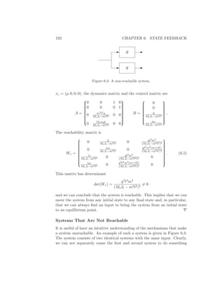
225. 6.6. FURTHER READING 213
To choose specific values for the cost function weights Qx and Qu, we
must use our knowledge of the system we are trying to control. A particu-
larly simple choice of weights is to use diagonal weights
Qx =


q1 0 · · ·
...
0 · · · qn


Qu = ρ


r1 0 · · ·
...
· · · 0 rn


.
For this choice of Qx and Qu, the individual diagonal elements describe how
much each state and input (squared) should contribute to the overall cost.
Hence, we can take states that should remain very small and attach higher
weight values to them. Similarly, we can penalize an input versus the states
and other inputs through choice of the corresponding input weight.
6.6 Further Reading
The importance of state models and state feedback was discussed in the
seminal paper by Kalman [Kal60] where the state feedback gain was obtained
by solving an optimization problem that minimized a quadratic loss function.
The notions of reachability and observability (next chapter) are also due to
Kalman [Kal61b];see also [Gil63, KHN63]. We note that in most textbooks
the term “controllability” is used instead of “reachability”, but we prefer
the latter term because it is more descriptive of the fundamental property
of being able to reach arbitrary states.
Most undergraduate textbooks on control will contain material on state
space systems, including, for example, Franklin, Powell and Emami-Naeini [FPEN05]
and Ogata [Oga01]. Friedland’s textbook [Fri04] covers the material in the
previous, current and next chapter in considerable detail, including the topic
of optimal control.
6.7 Exercises
1. Consider the system shown in Figure 6.3. Write the dynamics of the
two systems as
dx
dt
= Ax + Bu
dz
dt
= Az + Bu.

226. 214 CHAPTER 6. STATE FEEDBACK
Observe that if x and z have the same initial condition, they will
always have the same state, regardless of the input that is applied.
Show that this violates the definition of reachability and further show
that the reachability matrix Wr is not full rank.
2. Show that the characteristic polynomial for a system in reachable
canonical form is given by equation (6.7).
3. Consider a system on reachable canonical form. Show that the inverse
of the reachability matrix is given by
˜W−1
r =


1 a1 a2 · · · an
0 1 a1 · · · an−1
...
0 0 0 · · · 1


(6.26)
4. Extend the argument in Section 6.1 to show that if a system is reach-
able from an initial state of zero, it is reachable from a non-zero initial
state.
5. Build a simulation for the speed controller designed in Example 6.9
and show that with kr = 0, the system still achieves zero steady state
error.
6. Show that integral feedback can be used to compensate for a constant
disturbance by giving zero steady state error even when d = 0.
7. Show that if y(t) is the output of a linear system corresponding to
input u(t), then the output corresponding to an input ˙u(t) is given by
˙y(t). (Hint: use the definition of the derivative: ˙y(t) = limǫ→0 y(t +
ǫ) − y(t) /ǫ.)

227. Chapter 7
Output Feedback
There are none.
Abstract for “Gauranteed Margins for LQG Regulators”, John Doyle, 1978 [Doy78].
In the last chapter we considered the use of state feedback to modify
the dynamics of a system through feedback. In many applications, it is not
practical to measure all of the states directly and we can measure only a
small number of outputs (corresponding to the sensors that are available).
In this chapter we show how to use output feedback to modify the dynamics
of the system, through the use of observers (also called “state estimators”).
We introduce the concept of observability and show that if a system is
observable, it is possible to recover the state from measurements of the
inputs and outputs to the system.
7.1 Observability
In Section 6.2 of the previous chapter it was shown that it is possible to
find a feedback that gives desired closed loop eigenvalues provided that the
system is reachable and that all states are measured. For many situations,
it is highly unrealistic to assume that all states are measured. In this section
we will investigate how the state can be estimated by using a mathematical
model and a few measurements. It will be shown that the computation of
the states can be done by a dynamical system called an observer.
Consider a system described by
dx
dt
= Ax + Bu
y = Cx + Du,
(7.1)
215

228. 216 CHAPTER 7. OUTPUT FEEDBACK
Σ
Process
n
ˆxy
Observer
˙x = Ax + Bu
y = Cx + Du
u
Figure 7.1: Block diagram for an observer.
where x ∈ Rn is the state, u ∈ R the input, and y ∈ R the measured output.
We wish to estimate the state of the system from its inputs and outputs, as
illustrated in Figure 7.1. We assume that there is only one measured signal,
i.e. that the signal y is a scalar and that C is a (row) vector. This signal
may be corrupted by noise, n, although we shall start by considering the
noise-free case. We write ˆx for the state estimate given by the observer.
Definition 7.1 (Observability). A linear system is observable if for any
T > 0 it is possible to determine the state of the system x(T) through
measurements of y(t) and u(t) on the interval [0, T].
The problem of observability is one that has many important applica-
tions, even outside of feedback systems. If a system is observable, then there
are no “hidden” dynamics inside it; we can understand everything that is
going on through observation (over time) of the inputs and outputs. As
we shall see, the problem of observability is of significant practical interest
because it will tell if a set of sensors are sufficient for controlling a system.
Sensors combined with a mathematical model can also be viewed as a “vir-
tual sensor” that gives information about variables that are not measured
directly. The definition above holds for nonlinear systems as well, and the
results discussed here have extensions to the nonlinear case.
When discussing reachability in the last chapter we neglected the output
and focused on the state. Similarly, it is convenient here to initially neglect
the input and focus on the system
dx
dt
= Ax
y = Cx.
(7.2)
We wish to understand when it is possible to determine the state from
observations of the output.

229. 7.1. OBSERVABILITY 217
The output itself gives the projection of the state on vectors that are
rows of the matrix C. The observability problem can immediately be solved
if the matrix C is invertible. If the matrix is not invertible we can take
derivatives of the output to obtain
dy
dt
= C
dx
dt
= CAx.
From the derivative of the output we thus get the projection of the state on
vectors which are rows of the matrix CA. Proceeding in this way we get


y
˙y
¨y
...
y(n−1)


=


C
CA
CA2
...
CAn−1


x. (7.3)
We thus find that the state can be determined if the matrix
Wo =


C
CA
CA2
...
CAn−1


(7.4)
has n independent rows. It turns out that we need not consider any deriva-
tives higher than n − 1 (this is an application of the Cayley-Hamilton theo-
rem [Str88]).
The calculation can easily be extended to systems with inputs. The state
is then given by a linear combination of inputs and outputs and their higher
derivatives. We leave this as an exercise for the reader.
In practice, differentiation can give very large errors when there is mea-
surement noise and therefore the method sketched above is not particularly
practical. We will address this issue in more detail in the next section, but
for now we have the following basic result:
Theorem 7.1. A linear system of the form (7.1) is observable if and only
if the observability matrix Wo is full rank.
Proof. The sufficiency of the observability rank condition follows from the
analysis above. To prove necessity, suppose that the system is observable

230. 218 CHAPTER 7. OUTPUT FEEDBACK
but Wo is not full rank. Let v ∈ Rn, v = 0 be a vector in the null space of Wo,
so that Wov = 0. If we let x(0) = v be the initial condition for the system
and choose u = 0, then the output is given by y(t) = CeAtv. Since eAt can
be written as a power series in A and since An and higher powers can be
rewritten in terms of lower powers of A (by the Cayley-Hamilton theorem),
it follows that the output will be identically zero (the reader should fill in
the missing steps if this is not clear). However, if both the input and output
of the system are 0, then a valid estimate of the state is ˆx = 0 for all time,
which is clearly incorrect since x(0) = v = 0. Hence by contradiction we
must have that Wo is full rank if the system is observable.
Example 7.1 (Bicycle dynamics). To demonstrate the concept of observ-
ability, we consider the bicycle system, introduced in Section 3.2. Consider
the linearized model for the dynamics in equation (3.5), which has the form
J
d2ϕ
dt2
−
Dv0
b
dδ
dt
= mghϕ +
mv2
0h
b
δ,
where ϕ is the tilt of the bicycle and δ is the steering angle. Taking the torque
on the handle bars as an input and the lateral deviation as the output, we
can write the dynamics in state space form as (Exercise 3.3)
d
dt


x1
x2

 =


0 mgh/J
1 0




x1
x2

 +


1
0

 u
y =

Dv0
bJ
mv2
0h
bJ

 x.
The observability of this system determines whether it is possible to deter-
mine the entire system state (tilt angle and tilt rate) from observations of
the input (steering angle) and output (vehicle position).
The observability matrix is
W0 =


Dv0
bJ
mv2
0h
bJ
mv2
0h
bJ
mgh
J
ó Dv0
bJ


and its determinant is
det Wo =
Dv0
bJ
2
mgh
J
−
mv2
0h
bJ
2
.

231. 7.1. OBSERVABILITY 219
+
S
S
Figure 7.2: A non-observable system.
Under most choices of parameters, the determinant will be nonzero and
hence the system is observable. However, if the parameters of the system
are chosen such that
mv0h
D
=
mgh
J
then we see that Wo becomes singular and the system is not observable.
This case is explored in more detail in the exercises. ∇
Example 7.2 (Unobservable systems). It is useful to have an understanding
of the mechanisms that make a system unobservable. Such a system is
shown in Figure 7.2. The system is composed of two identical systems whose
outputs are added. It seems intuitively clear that it is not possible to deduce
the states from the output since we cannot deduce the individual output
contributions from the sum. This can also be seen formally (Exercise 1). ∇
As in the case of reachability, certain canonical forms will be useful in
studying observability. We define the observable canonical form to be the
dual of the reachable canonical form.
Definition 7.2 (Observable canonical form). A linear state space system is
in observable canonical form if its dynamics are given by
dz
dt
=


−a1 1 0 · · · 0
−a2 0 1 0
...
...
−an−1 0 0 1
−an 0 0 · · · 0


z +


b1
b2
...
bn−1
bn


u
y =

1 0 0 · · · 0

 z + Du.
Figure 7.3 shows a block diagram for a system in observable canonical
form. As in the case of reachable canonical form, we see that the coeffi-

232. 220 CHAPTER 7. OUTPUT FEEDBACK
Σ
an
u
bn
. . .
. . .
an−1
bn−1
Σ Σ
. . .
a2
b2
−1
y
a1
b1
ΣΣ
Figure 7.3: Block diagram of a system on observable canonical form.
cients in the system description appear directly in the block diagram. The
characteristic equation for a system in observable canonical form is given by
λ(s) = sn
+ a1sn−1
+ · · · + an−1s + an. (7.5)
It is possible to reason about the observability of a system in observable
canonical form by studying the block diagram. If the input u and the out-
put are available the state x1 can clearly be computed. Differentiating x1
we also obtain the input to the integrator that generates x1 and we can
now obtain x2 = ˙x1 + a1x1 − b1u. Proceeding in this way we can clearly
compute all states. The computation will however require that the signals
are differentiated.
We can now proceed with a formal analysis. The observability matrix
for a system in observable canonical form is given by
Wo =


1 0 0 . . . 0
−a1 1 0 . . . 0
−a2
1 − a1a2 −a1 1 . . . 0
...
...
...
∗ . . . 1


,
where * represents as entry whose exact value is not important. The rows of
this matrix are linearly independent (since it is lower triangular) and hence
Wo is full rank. A straightforward but tedious calculation shows that the

233. 7.2. STATE ESTIMATION 221
inverse of the observability matrix has a simple form, given by
W−1
o =


1 0 0 · · · 0
a1 1 0 · · · 0
a2 a1 1 · · · 0
...
...
an−1 an−2 an−3 · · · 1


.
As in the case of reachability, it turns out that if a system is observable
then there always exists a transformation T that converts the system into
reachable canonical form (Exercise 3). This is very useful for proofs, since
it lets us assume that a system is in reachable canonical form without any
loss of generality.
7.2 State Estimation
Having defined the concept of observability, we now return to the question
of how to construct an observer for a system. We will look for observers
that can be represented as a linear dynamical system that takes the inputs
and outputs of the system we are observing and produces an estimate of
the system’s state. That is, we wish to construct a dynamical system of the
form
dˆx
dt
= F ˆx + Gu + Hy,
where u and y are the input and output of the original system and ˆx ∈ Rn
is an estimate of the state with the property that ˆx(t) → x(t) as t → ∞.
The Basic Observer
For a system governed by equation (7.1), we can attempt to determine the
state simply by simulating the equations with the correct input. An estimate
of the state is then given by
dˆx
dt
= Aˆx + Bu. (7.6)
To find the properties of this estimate, introduce the estimation error
˜x = x − ˆx.
It follows from equations (7.1) and (7.6) that
d˜x
dt
= A˜x.

234. 222 CHAPTER 7. OUTPUT FEEDBACK
If matrix A has all its eigenvalues in the left half plane, the error ˜x will thus
go to zero and hence equation (7.6) is a dynamical system whose output
converges to the state of the system (7.1).
The observer given by equation (7.6) uses only the process input u; the
measured signal does not appear in the equation. We must also require
that the system is stable and essentially our estimator converges because
the state of both the observer and the estimator are going zero. This is not
very useful in a control design context since we want to have our estimate
converge quickly to a nonzero state, so that we can make use of it in our
controller. We will therefore attempt to modify the observer so that the
output is used and its convergence properties can be designed to be fast
relative to the system’s dynamics. This version will also work for unstable
systems.
Consider the observer
dˆx
dt
= Aˆx + Bu + L(y − Cˆx). (7.7)
This can be considered as a generalization of equation (7.6). Feedback from
the measured output is provided by adding the term L(y − Cˆx), which is
proportional to the difference between the observed output and the output
that is predicted by the observer. To investigate the observer (7.7), form
the error ˜x = x − ˆx. It follows from equations (7.1) and (7.7) that
d˜x
dt
= (A − LC)˜x.
If the matrix L can be chosen in such a way that the matrix A − LC has
eigenvalues with negative real parts, the error ˜x will go to zero. The con-
vergence rate is determined by an appropriate selection of the eigenvalues.
The problem of determining the matrix L such that A − LC has pre-
scribed eigenvalues is very similar to the eigenvalue assignment problem that
was solved in the previous chapter. In fact, since the eigenvalues of the ma-
trix and its transpose are the same, it is equivalent to search for LT such
that AT −CT LT has the desired eigenvalues. This is precisely the eigenvalue
assignment problem that we solved in the previous chapter, with ˜A = AT ,
˜B = CT and ˜K = LT . Thus, using the results of Theorem 6.3, we can have
the following theorem on observer design:
Theorem 7.2 (Observer design by eigenvalue assignment). Consider the
system given by
dx
dt
= Ax + Bu
y = Cx
(7.8)

235. 7.2. STATE ESTIMATION 223
with one input and one output. Let λ(s) = sn + a1sn−1 + · · · + an−1s + an
be the characteristic polynomial for A. If the system is observable then the
dynamical system
dˆx
dt
= Aˆx + Bu + L(y − Cˆx) (7.9)
is an observer for the system, with L chosen as
L = W−1
o
˜Wo


p1 − a1
p2 − a2
...
pn − an


, (7.10)
and the matrices Wo and ˜Wo given by
Wo =


C
CA
...
CAn−1


˜Wo =


1 0 0 · · · 0
a1 1 0 · · · 0
a2 a1 1 · · · 0
...
an−1 an−2 an−3 · · · 1


−1
.
The resulting observer error ˜x = x − ˆx is governed by a differential equation
having the characteristic polynomial
p(s) = sn
+ p1sn−1
+ · · · + pn.
The dynamical system (7.9) is called an observer for (the states of) the
system (7.8) because it will generate an approximation of the states of the
system from its inputs and outputs. This particular form of an observer
is a much more useful form than the one given by pure differentiation in
equation (7.3).
Interpretation of the Observer
The observer is a dynamical system whose inputs are the process input u
and process output y. The rate of change of the estimate is composed of two
terms. One term, Aˆx + Bu, is the rate of change computed from the model
with ˆx substituted for x. The other term, L(y − ˆy), is proportional to the
difference e = y − ˆy between measured output y and its estimate ˆy = Cˆx.
The estimator gain L is a matrix that tells how the error e is weighted and
distributed among the states. The observer thus combines measurements

236. 224 CHAPTER 7. OUTPUT FEEDBACK
ˆx
˙ˆxu
ˆyy
B Σ
Σ
A
C
−1
L
Figure 7.4: Block diagram of the observer. Notice that the observer contains a copy
of the process.
with a dynamical model of the system. A block diagram of the observer is
shown in Figure 7.4.
Notice the similarity between the problems of finding a state feedback
and finding the observer. The key is that both of these problems are equiva-
lent to the same algebraic problem. In eigenvalue assignment it is attempted
to find K so that A − BK has given eigenvalues. For the observer design it
is instead attempted to find L so that A − LC has given eigenvalues. The
following equivalence can be established between the problems:
A ↔ AT
B ↔ CT
K ↔ LT
Wr ↔ WT
o
The observer design problem is often called the dual of the state feedback de-
sign problem. The similarity between design of state feedback and observers
also means that the same computer code can be used for both problems.
Computing the Observer Gain
The observer gain can be computed in several different ways. For simple
problems it is convenient to introduce the elements of L as unknown param-
eters, determine the characteristic polynomial of the observer and identify it
with the desired characteristic polynomial. Another alternative is to use the
fact that the observer gain can be obtained by inspection if the system is in
observable canonical form. The observer gain is then obtained by transfor-
mation to the canonical form. There are also reliable numerical algorithms,

237. 7.2. STATE ESTIMATION 225
which are identical to the algorithms for computing the state feedback. The
procedures are illustrated by example.
Example 7.3 (Vehicle steering). Consider the normalized, linear model for
vehicle steering in Example 5.12. The dynamics relating steering angle u to
lateral path deviation y is given by the state space model
dx
dt
=


0 1
0 0

 x +


α
1

 u
y =

1 0

 x.
(7.11)
Recall that the state x1 represents the lateral path deviation and that x2
represents turning rate. We will now derive an observer that uses the system
model to determine turning rate from the measured path deviation.
The observability matrix is
Wo =


1 0
0 1

 ,
i.e., the identity matrix. The system is thus observable and the eigenvalue
assignment problem can be solved. We have
A − LC =


−l1 1
−l2 0

 ,
which has the characteristic polynomial
det (sI − A + LC) = det


s + l1 −1
l2 s

 = s2
+ l1s + l2.
Assuming that it is desired to have an observer with the characteristic poly-
nomial
s2
+ p1s + p2 = s2
+ 2ζoωos + ω2
o,
the observer gains should be chosen as
l1 = p1 = 2ζoωo
l2 = p2 = ω2
o.
The observer is then
dˆx
dt
= Aˆx + Bu + L(y = Cx) =


0 1
0 0

 ˆx +


0
1

 u +


l1
l2

 (y − ˆx1).
∇

238. 226 CHAPTER 7. OUTPUT FEEDBACK
For larger systems, the place or acker commands can be used in MAT-
LAB. Note that these functions are the same as the ones used for eigenvalue
assignment with state feedback; for estimator design, one simply uses the
transpose of the dynamics matrix and the output matrix.
7.3 Control using Estimated State
In this section we will consider the same system as in the previous sections,
i.e., the state space system described by
dx
dt
= Ax + Bu
y = Cx.
(7.12)
We wish to design a feedback controller for the system where only the output
is measured. As before, we will be assume that u and y are scalars. We also
assume that the system is reachable and observable. In Chapter 6 we found
a feedback of the form
u = Kx + krr
for the case that all states could be measured and in Section 7.2 we have
developed an observer that can generate estimates of the state ˆx based
on inputs and outputs. In this section we will combine the ideas of these
sections to find a feedback that gives desired closed loop eigenvalues for
systems where only outputs are available for feedback.
If all states are not measurable, it seems reasonable to try the feedback
u = −Kˆx + krr (7.13)
where ˆx is the output of an observer of the state, i.e.
dˆx
dt
= Aˆx + Bu + L(y − Cˆx). (7.14)
Since the system (7.12) and the observer (7.14) both are of state dimen-
sion n, the closed loop system has state dimension 2n. The states of the
combined system are x and ˆx. The evolution of the states is described by
equations (7.12), (7.13) and (7.14). To analyze the closed loop system, the
state variable ˆx is replaced by
˜x = x − ˆx. (7.15)

239. 7.3. CONTROL USING ESTIMATED STATE 227
Subtraction of equation (7.14) from equation (7.12) gives
d˜x
dt
= Ax − Aˆx − L(y − Cˆx) = A˜x − LC˜x = (A − LC)˜x.
Returning to the process dynamics, introducing u from equation (7.13)
into equation (7.12) and using equation (7.15) to eliminate ˆx gives
dx
dt
= Ax + Bu = Ax − BKˆx + Bkrr = Ax − BK(x − ˜x) + Bkrr
= (A − BK)x + BK˜x + Bkrr.
The closed loop system is thus governed by
d
dt


x
˜x

 =


A − BK BK
0 A − LC




x
˜x

 +


Bkr
0

 r. (7.16)
Notice that the state ˜x, representing the observer error, is not affected by
the command signal r. This is desirable since we do not want the reference
signal to generate observer errors.
Since the dynamics matrix is block diagonal, we find that the character-
istic polynomial of the closed loop system is
λ(s) = det (sI − A + BK) det (sI − A + LC).
This polynomial is a product of two terms: the characteristic polynomial of
the closed loop system obtained with state feedback and the characteristic
polynomial of the observer error. The feedback (7.13) that was motivated
heuristically thus provides a very neat solution to the eigenvalue assignment
problem. The result is summarized as follows.
Theorem 7.3 (Eigenvalue assignment by output feedback). Consider the
system
dx
dt
= Ax + Bu
y = Cx.
The controller described by
u = −Kˆx + krr
dˆx
dt
= Aˆx + Bu + L(y − Cˆx)

240. 228 CHAPTER 7. OUTPUT FEEDBACK
r u yx˙x
ˆx
−ˆy
B
B
Σ
Σ
Σ
Σ
R
R
A
A
C
−C
L
−K
kr
Process
Observer
Figure 7.5: Block diagram of a control system that combines state feedback with
an observer.
gives a closed loop system with the characteristic polynomial
λ(s) = det (sI − A + BK) det (sI − A + LC).
This polynomial can be assigned arbitrary roots if the system is reachable
and observable.
The controller has a strong intuitive appeal: it can be thought of as
composed of two parts, one state feedback and one observer. The feedback
gain K can be computed as if all state variables can be measured. This
property is called the separation principle and it allows us to independently
solve for the state space controller and the state space estimator.
A block diagram of the controller is shown in Figure 7.5. Notice that
the controller contains a dynamical model of the plant. This is called the
internal model principle: the controller contains a model of the process being
controlled. Indeed, the dynamics of the controller is due to the observer and
can thus be viewed as a dynamical system with input y and output u:
dˆx
dt
= (A − BK − LC)ˆx + Ly
u = −Kˆx + krr.
(7.17)

241. 7.4. KALMAN FILTERING 229
Example 7.4 (Vehicle steering). Consider again the normalized, linear
model for vehicle steering in Example 5.12. The dynamics relating steering
angle u to lateral path deviation y is given by the state space model (7.11).
Combining the state feedback derived in Example 6.4 with the observer
determined in Example 7.3 we find that the controller is given by
dˆx
dt
= Aˆx + Bu + L(y − Cx) =


0 1
0 0

 ˆx +


0
1

 u +


l1
l2

 (y − ˆx1)
u = −Kˆx + krr = k1(r − x1) − k2x2
The controller is thus a dynamical system of second order. Elimination of
the variable u gives
dˆx
dt
= (A − BK − LC)ˆx + Ly + Bkrr
=


−l1 − αk1 1 − αk2
−k1 − l2 −k2

 ˆx +


l1
l2

 y +


α
1

 k1r
u = −Kˆx + krr = −

k1 k2

 ˆx + k1r.
The controller is a dynamical system of second order, with two inputs y and
r and one output u. ∇
7.4 Kalman Filtering
One of the principal uses of observers in practice is to estimate the state of
a system in the presence of noisy measurements. We have not yet treated
noise in our analysis and a full treatment of stochastic dynamical systems is
beyond the scope of this text. In this section, we present a brief introduction
to the use of stochastic systems analysis for constructing observers. We work
primarily in discrete time to avoid some of the complications associated
with continuous time random processes and to keep the mathematical pre-
requisites to a minimum. This section assumes basic knowledge of random
variables and stochastic processes.
Consider a discrete time, linear system with dynamics
xk+1 = Axk + Buk + Fvk
yk = Cxk + wk,
(7.18)

242. 230 CHAPTER 7. OUTPUT FEEDBACK
where vk and wk are Gaussian, white noise processes satisfying
E{vk} = 0 E{wk} = 0
E{vkvT
j } =
0 k = j
Rv k = j
E{wkwT
j } =
0 k = j
Rw k = j
E{vkwT
j } = 0.
(7.19)
We assume that the initial condition is also modeled as a Gaussian random
variable with
E{x0} = x0 E{x0xT
0 } = P0. (7.20)
We wish to find an estimate ˆxk that minimizes the mean square error
E{(xk − ˆxk)(xk − ˆxk)T } given the measurements {y(δ) : 0 ≤ τ ≤ t}. We
consider an observer in the same basic form as derived previously:
ˆxk+1 = Aˆxk + Buk + Lk(yk − Cˆxk). (7.21)
The following theorem summarizes the main result.
Theorem 7.4. Consider a random process xk with dynamics (7.18) and
noise processes and initial conditions described by equations (7.19) and (7.20).
The observer gain L that minimizes the mean square error is given by
Lk = AT
PkCT
(Rw + CPkCT
)−1
,
where
Pk+1 = (A − LC)Pk(A − LC)T
+ Rv + LRwLT
P0 = E{X(0)XT
(0)}.
(7.22)
Before we prove this result, we reflect on its form and function. First,
note that the Kalman filter has the form of a recursive filter: given Pk =
E{EkET
k } at time k, can compute how the estimate and covariance change.
Thus we do not need to keep track of old values of the output. Furthermore,
the Kalman filter gives the estimate ˆxk and the covariance PE,k, so we can
see how reliable the estimate is. It can also be shown that the Kalman filter
extracts the maximum possible information about output data. If we form
the residual between the measured output and the estimated output,
ek = yk − Cˆxk,
we can can show that for the Kalman filter the correlation matrix is
Re(j, k) = Wδjk.

243. 7.4. KALMAN FILTERING 231
In other words, the error is a white noise process, so there is no remaining
dynamic information content in the error.
In the special case when the noise is stationary (Q, R constant) and if
Pk converges, then the observer gain is constant:
K = AT
PCT
(Rw + CPCT
),
where
P = APAT
+ Rv − APCT
Rw + CPCT −1
CPAT
.
We see that the optimal gain depends on both the process noise and the
measurement noise, but in a nontrivial way. Like the use of LQR to choose
state feedback gains, the Kalman filter permits a systematic derivation of
the observer gains given a description of the noise processes. The solution
for the constant gain case is solved by the dlqe command in MATLAB.
Proof (of theorem). We wish to minimize the mean square of the error,
E{(xk − ˆxk)(xk − ˆxk)T }. We will define this quantity as Pk and then show
that it satisfies the recursion given in equation (7.22). By definition,
Pk+1 = E{xk+1xT
k+1}
= (A − LC)Pk(A − LC)T
+ Rv + LRwLT
= APkAT
− APkCT
LT
− LCAT
+ L(Rw + CPkCT
)LT
Letting Rǫ = (Rw + CPkCT ), we have
Pk+1 = APkAT
− APkCT
LT
− LCAT
+ LRǫLT
= APkAT
+ L − APkCT
R−1
ǫ Rǫ L − APKCT
R−1
ǫ
T
− APkCT
R−1
ǫ CPT
k AT
+ Rw.
In order to minimize this expression, we choose L = APkCT R−1
ǫ and the
theorem is proven.
The Kalman filter can also be applied to continuous time stochastic pro-
cesses. The mathematical derivation of this result requires more sophisti-
cated tools, but the final form of the estimator is relatively straightforward.
Consider a continuous stochastic system
˙x = Ax + Bu + Fv E{v(s)vT
(t)} = Q(t)δ(t − s)
y = Cx + w E{w(s)wT
(t)} = R(t)δ(t − s)

244. 232 CHAPTER 7. OUTPUT FEEDBACK
Assume that the disturbance v and noise w are zero-mean and Gaussian
(but not necessarily stationary):
pdf(v) =
1
n
√
2π
√
det Q
e− 1
2
vT Q−1v
pdf(w) = . . . (using R)
We wish to find the estimate ˆx(t) that minimizes the mean square error
E{(x(t) − ˆx(t))(x(t) − ˆx(t))T } given {y(τ) : 0 ≤ τ ≤ t}.
Theorem 7.5 (Kalman-Bucy, 1961). The optimal estimator has the form
of a linear observer
˙ˆx = Aˆx + Bu + L(y − Cˆx)
where L(t) = P(t)CT R−1 and P(t) = E{(x(t) − ˆx(t))(x(t) − ˆx(t))T } and
satisfies
˙P = AP + PAT
− PCT
R−1
(t)CP + FQ(t)FT
P(0) = E{x(0)xT
(0)}
7.5 State Space Control Systems
In this section we consider a collection of additional topics on the design
and analysis of control systems using state space tools.
Computer Implementation
The controllers obtained so far have been described by ordinary differential
equations. They can be implemented directly using analog components,
whether electronic circuits, hydraulic valves or other physical devices. Since
in modern engineering applications most controllers are implemented using
computers we will briefly discuss how this can be done.
A computer controlled system typically operates periodically: every cy-
cle, signals from the sensors are sampled and converted to digital form by
the A/D converter, the control signal is computed, and the resulting output
is converted to analog form for the actuators (as shown in Figure 1.3 on
page 5). To illustrate the main principles of how to implement feedback in
this environment, we consider the controller described by equations (7.13)
and (7.14), i.e.,
u = −Kˆx + krr
dˆx
dt
= Aˆx + Bu + K(y − Cˆx).

245. 7.5. STATE SPACE CONTROL SYSTEMS 233
The first equation consists only of additions and multiplications and can
thus be implemented directly on a computer. The second equation has
to be approximated. A simple way is to approximate the derivative by a
difference
dx
dt
≈
ˆx(tk+1) − ˆx(tk)
h
= Aˆx(tk) + Bu(tk) + K(y(tk) − Cˆx(tk))
where tk are the sampling instants and h = tk+1 −tk is the sampling period.
Rewriting the equation to isolate x(tk+1), we get
ˆx(tk+1) = ˆx(tk) + h Aˆx(tk) + Bu(tk) + K(y(tk) − Cˆx(tk)) . (7.23)
The calculation of the estimated state at time tk+1 only requires addition
and multiplication and can easily be done by a computer. A section of
pseudo code for the program that performs this calculation is
% Control algorithm - main loop
r = adin(ch1) % read setpoint from ch1
y = adin(ch2) % get process output from ch2
u = C*xhat + Kr*r % compute control variable
daout(ch1, u) % set analog output on ch1
xhat = xhat + h*(A*x+B*u+L*(y-C*x)) % update state estimate
The program runs periodically at a fixed rate h. Notice that the number
of computations between reading the analog input and setting the analog
output has been minimized. The state is updated after the analog output
has been set. The program has an array of states, xhat, that represents the
state estimate. The choice of sampling period requires some care.
There are several practical issues that also must be dealt with. For ex-
ample it is necessary to filter a signal before it is sampled so that the filtered
signal has little frequency content above fs/2 where fs is the sampling fre-
quency. If controllers with integral action are used, it is also necessary to
provide protection so that the integral does not become too large when the
actuator saturates. This issue, called integrator windup, is studied in more
detail in Chapter 10. Care must also be taken so that parameter changes
do not cause disturbances.
A General Controller Structure
We now consider a general control structure that pulls together the various
results the the previous and current chapters. This structure is one that
appears in may places in control theory and is the heart of most modern
control systems.

246. 234 CHAPTER 7. OUTPUT FEEDBACK
Trajectory
Generator
r
u
-ˆx
xd
ProcessΣ Σ
State
Feedback
Observer
ufb
ud
y
Figure 7.6: Block diagram of a controller based on a structure with two degrees
of freedom. The controller consists of a command signal generator, state feedback
and an observer.
We begin by generalizing the way we handle the reference input. So
far reference signals have been introduced simply by adding them to the
state feedback through a gain kr. A more sophisticated way of doing this
is shown by the block diagram in Figure 7.6, where the controller consists
of three parts: an observer that computes estimates of the states based on
a model and measured process inputs and outputs, a state feedback and
a trajectory generator that generates the desired behavior of all states xd
and a feedforward signal ud. The signal ud is such that it generates the
desired behavior of the states when applied to the system, under the ideal
conditions of no disturbances and no modeling errors. The controller is said
to have two degrees of freedom because the response to command signals
and disturbances are decoupled. Disturbance responses are governed by the
observer and the state feedback and the response to command signals is
governed by the trajectory generator (feedfoward).
We start with the full nonlinear dynamics of the process
˙x = f(x, u)
y = h(x, u).
(7.24)
Assume that the trajectory generator is able to generate a desired trajectory
(xd, ud) that satisfies the dynamics (7.24) and satisfies r = h(xd, ud). To
design the controller, we construct the error system. We will assume for
simplicity that f(x, u) = f(x) + g(x)u (i.e., the system is nonlinear in the
state, but linear in the input; this is often the case in applications). Let

247. 7.5. STATE SPACE CONTROL SYSTEMS 235
e = x − xd, v = u − ud and compute the dynamics for the error:
˙e = ˙x − ˙xd = f(x) + g(x)u − f(xd) + g(xd)ud
= f(e + xd) − f(xd) + g(e + xd)(v + ud) − g(xd)ud
= F(e, v, xd(t), ud(t))
In general, this system is time varying.
For trajectory tracking, we can assume that e is small (if our controller
is doing a good job) and so we can linearize around e = 0:
˙e ≈ A(t)e + B(t)v
where
A(t) =
∂F
∂e (xd(t),ud(t))
B(t) =
∂F
∂v (xd(t),ud(t)
.
It is often the case that A(t) and B(t) depend only on xd, in which case it
is convenient to write A(t) = A(xd) and B(t) = B(xd).
Assume now that xd and ud are either constant or slowly varying (with
respect to the performance criterion). This allows us to consider just the
(constant) linear system given by (A(xd), B(xd)). If we design a state feed-
back controller K(xd) for each xd, then we can regulate the system using
the feedback
v = K(xd)e.
Substituting back the definitions of e and v, our controller becomes
u = K(xd)(x − xd) + ud
This form of controller is called a gain scheduled linear controller with feed-
forward ud.
Finally, we consider the observer. We can use the full nonlinear dynamics
for the prediction portion of the observer and the linearized system for the
correction term:
˙ˆx = f(ˆx, u) + L(ˆx)(y − h(ˆx, u))
where L(ˆx) is the observer gain obtained by linearizing the system around
the currently estimate state. This form of the observer is known as an
extended Kalman filter and has proven to be a very effective means of esti-
mating the state of a nonlinear system.
To get some insight into the overall behavior of the system, we consider
what happens when the command signal is changed. To fix the ideas let us
assume that the system is in equilibrium with the observer state ˆx equal to

248. 236 CHAPTER 7. OUTPUT FEEDBACK
the process state x. When the command signal is changed a feedforward
signal ud(t) is generated. This signal has the property that the process
output gives the desired state xd(t) when the feedforward signal is applied
to the system. The process state changes in response to the feedforward
signal. The observer tracks the state perfectly because the initial state was
correct. The estimated state ˆx will thus be equal to the desired state xd and
the feedback signal L(xd − ˆx) is zero. If there are some disturbances or some
modeling errors the feedback signal will be different from zero and attempt
to correct the situation.
The controller given in Figure 7.6 is a very general structure. There
are many ways to generate the feedforward signal and there are also many
different ways to compute the feedback gain K and the observer gain L.
Note that once again the internal model principle applies: the controller
contains a model of the system to be controlled.
The Kalman Decomposition
In this chapter and the previous one, we have seen that two fundamental
properties of a linear input/output system are reachability and observability.
It turns out that these two properties can be used to classify the dynamics
of a system. The key result is Kalman’s decomposition theorem, which
says that a linear system can be divided into four subsystems: Sro which
is reachable and observable, Sr¯o which is reachable but not observable, S¯ro
which is not reachable but is observable, and S¯r¯o which is neither reachable
nor observable.
We will first consider this in the special case of systems where the matrix
A has distinct eigenvalues. In this case we can find a set of coordinates such
that the A matrix is diagonal and, with some additional reordering of the
states, the system can be written as
dz
dt
=


Λro 0 0 0
0 Λr¯o 0 0
0 0 Λ¯ro 0
0 0 0 Λ¯r¯o


z +


βro
βro
0
0


u
y =

γro 0 γ¯ro 0

 z + Du.
All states zk such that βk = 0 are controllable and all states such that γk = 0
are observable. The frequency response of the system is given by
G(s) = γro(sI − Aro)−1
βro + D

249. 7.5. STATE SPACE CONTROL SYSTEMS 237
Figure 7.7: Kalman’s decomposition of a linear system with distinct eigenvalues.
and it is uniquely given by the subsystem that is reachable and observable.
Thus from the input/output point of view, it is only the reachable and
observable dynamics that matter. A block diagram of the system illustrating
this property is given in Figure 7.7.
The general case of the Kalman decomposition is more complicated and
requires some additional linear algebra. Introduce the reachable subspace
Xr which is the linear subspace spanned by the columns of the reachability
matrix Wr. The state space is the direct sum of Xr and another linear
subspace X¯r. Notice that Xr is unique but that X¯r can be chosen in many
different ways. Choosing coordinates with xr ∈ Xr and x¯r ∈ X¯r the system
equations can be written as
d
dt


xr
x¯r

 =


A11 A12
0 A22




xr
x¯r

 +


B1
0

 u, (7.25)
where the states xr are reachable and x¯r are non-reachable.
Introduce the unique subspace X¯o of non-observable states. This is the
right null space of the observability matrix Wo. The state space is the direct
sum of X¯o and the non-unique subspace Xo. Choosing a coordinate system
with xo ∈ Xo and x¯o ∈ X¯o the system equations can be written as
d
dt


xo
x¯o

 =


A11 0
A21 A22




xo
x¯o


y =

C1 0




xo
x¯o

 ,
(7.26)

250. 238 CHAPTER 7. OUTPUT FEEDBACK
Figure 7.8: Kalman’s decomposition of a linear system with general eigenvalues.
where the states xo are observable and x¯o are not observable.
The intersection of two linear subspaces is also a linear subspace. In-
troduce Xr¯o as the intersection of Xr and X¯o and the complementary linear
subspace Xro, which together with Xr¯o spans Xr. Finally, we introduce the
linear subspace X¯ro which together with Xr¯o, Xr¯o and Xr¯o spans the full
state space. Notice that the decomposition is not unique because only the
subspace Xr¯o is unique.
Combining the representations (7.25) and (7.26) we find that a linear
system can be transformed to the form
dx
dt
=


A11 0 A13 0
A21 A22 A23 A24
0 0 A33 0
0 0 A43 A44


x +


B1
B2
0
0


u
y =

C1 0 C2 0

 x,
(7.27)
where the state vector has been partitioned as
x =


xro
xr¯o
x¯ro
x¯r¯o


A block diagram of the system is shown in Figure 7.8. By tracing the
arrows in the diagram we find that the input influences the systems Sro and

251. 7.6. FURTHER READING 239
S¯ro and that the output is influenced by Sro and S¯ro. The system S¯r¯o is
neither connected to the input nor the output. The frequency response of
the system is thus
G(s) = C1(sI − A11)−1
B1, (7.28)
which is the dynamics of the reachable and observable subsystem Sro.
7.6 Further Reading
The notion of observability is due to Kalman [Kal61b] and, combined with
the dual notion of reachability, it was a major stepping stone toward estab-
lishing state space control theory beginning in the 1960s. For linear systems
the output is a projection of the state and it may seem unnecessary to esti-
mate the full state since a projection is already available. Luenberger [Lue71]
constructed an reduced order observer that only reconstructs the state that
is not measured directly.
The main result of this chapter is the general controller structure in Fig-
ure 7.6. This controller structure emerged as a result of solving optimization
problems. The observer first appeared as the Kalman filter which was also
the solution to an optimization problem [Kal61a, KB61]. It was then shown
that the solution to an optimization with output feedback could be obtained
by combining a state feedback with a Kalman filter [JT61, GF71]. Later
it was found that the controller with the same structure also emerged as
solutions of other simpler deterministic control problems like the ones dis-
cussed in this chapter [?, ?]. Much later it was shown that solutions to
robust control problems also had a similar structure but with different ways
of computing observer and state feedback gains [DGKF89]. The material is
now an essential part of the tools in control.
A more detailed presentation of stochastic control theory is given in [˚Ast70].
7.7 Exercises
1. Show that the system depicted in Figure 7.2 is not observable.
2. Consider a system under a coordinate transformation z = Tx, where
T ∈ Rn×n is an invertible matrix. Show that the observability ma-
trix for the transformed system is given by ˜Wo = WoT−1 and hence
observability is independent of the choice of coordinates.

252. 240 CHAPTER 7. OUTPUT FEEDBACK
3. Show that if a system is observable, then there exists a change of
coordinates z = Tx that puts the transformed system into reachable
canonical form.

253. Chapter 8
Transfer Functions
The typical regulator system can frequently be described, in essentials, by
differential equations of no more than perhaps the second, third or fourth
order. . . . In contrast, the order of the set of differential equations describing
the typical negative feedback amplifier used in telephony is likely to be very
much greater. As a matter of idle curiosity, I once counted to find out what
the order of the set of equations in an amplifier I had just designed would
have been, if I had worked with the differential equations directly. It turned
out to be 55.
Henrik Bode, 1960 [Bod60].
This chapter introduces the concept of the transfer function, which is a
compact description of the input/output relation for a linear system. Com-
bining transfer functions with block diagrams gives a powerful method for
dealing with complex linear systems. The relationship between transfer
functions and other system descriptions of dynamics is also discussed.
8.1 Frequency Domain Analysis
Figure 8.1 shows a block diagram for a typical control system, consisting of a
process to be controlled and a (dynamic) compensator, connected in a feed-
back loop. We saw in the previous two chapters how to analyze and design
such systems using state space descriptions of the blocks. As was mentioned
in Chapter 2, an alternative approach is to focus on the input/output char-
acteristics of the system. Since it is the inputs and outputs that are used to
connect the systems, one could expect that this point of view would allow
an understanding of the overall behavior of the system. Transfer functions
are the main tool in implementing this point of view for linear systems.
241

254. 242 CHAPTER 8. TRANSFER FUNCTIONS
−1
r ΣF P
yu
d n
C
e
reference feedback process
shaping controller dynamics
Σ Σ
Figure 8.1: A block diagram for a feedback control system.
The basic idea of the transfer function comes from looking at the fre-
quency response of a system. Suppose that we have an input signal that is
periodic. Then we can always decompose this signal into the sum of a set
of sines and cosines,
u(t) =
∞
k=1
ak sin(kωt) + bk cos(kωt),
where ω is the fundamental frequency of the periodic input. Each of the
terms in this input generates a corresponding sinusoidal output (in steady
state), with possibly shifted magnitude and phase. The magnitude gain and
phase at each frequency is determined by the frequency response, given in
equation (5.21):
G(s) = C(sI − A)−1
B + D, (8.1)
where we set s = j(kω) for each k = 1, . . . , ∞. If we know the steady
state frequency response G(s), we can thus compute the response to any
(periodic) signal using superposition.
The transfer function generalizes this notion to allow a broader class of
input signals besides periodic ones. As we shall see in the next section, the
transfer function represents the response of the system to an “exponential
input,” u = est. It turns out that the form of the transfer function is
precisely the same as equation (8.1). This should not be surprising since we
derived equation (8.1) by writing sinusoids as sums of complex exponentials.
Formally, the transfer function corresponds to the Laplace transform of the
steady state response of a system, although one does not have to understand
the details of Laplace transforms in order to make use of transfer functions.
The power of transfer functions is that they allow a particularly conve-
nient form for manipulating and analyzing complex feedback systems. As we
shall see, there are many graphical representations of transfer functions that

255. 8.2. DERIVATION OF THE TRANSFER FUNCTION 243
capture interesting properties of dynamics. Transfer functions also make it
possible to express the changes in a system because of modeling error, which
is essential when discussing sensitivity to process variations of the sort dis-
cussed in Chapter 12. In particular, using transfer functions it is possible
to analyze what happens when dynamic models are approximated by static
models or when high order models are approximated by low order models.
One consequence is that we can introduce concepts that express the degree
of stability of a system.
The main limitation of transfer functions is that they can only be used
for linear systems. While many of the concepts for state space modeling
and analysis extend to nonlinear systems, there is no such analog for trans-
fer functions and there are only limited extensions of many of the ideas
to nonlinear systems. Hence for the remainder of the text we shall limit
ourselves to linear models. However, it should be pointed out that despite
this limitation, transfer functions still remain a valuable tool for designing
controllers for nonlinear systems, chiefly through constructing their linear
approximations around an equilibrium point of interest.
8.2 Derivation of the Transfer Function
As we have seen in previous chapters, the input/output dynamics of a linear
system has two components: the initial condition response and the forced
response. In addition, we can speak of the transient properties of the system
and its steady state response to an input. The transfer function focuses on
the steady state response due to a given input, and provides a mapping
between inputs and their corresponding outputs. In this section, we will
derive the transfer function in terms of the “exponential response” of a
linear system.
Transmission of Exponential Signals
To formally compute the transfer function of a system, we will make use of
a special type of signal, called an exponential signal, of the form est where
s = σ +jω is a complex number. Exponential signals play an important role
in linear systems. They appear in the solution of differential equations and in
the impulse response of linear systems, and many signals can be represented
as exponentials or sums of exponentials. For example, a constant signal is
simply eαt with α = 0. Damped sine and cosine signals can be represented
by
e(σ+jω)t
= eσt
ejωt
= eσt
(cos ωt + i sin ωt),

256. 244 CHAPTER 8. TRANSFER FUNCTIONS
0 0.5 1
0
0.5
1
x
y
s=0
0 2 4
0
0.5
1
x
y
s=−1
0 0.5 1
0
1
2
3
x
y
s=1
0 5 10 15
−1
−0.5
0
0.5
1
x
y
z=0
0 5 10 15
−1
−0.5
0
0.5
1
x
y
z=0.2
0 5 10 15
−20
−10
0
10
20
x
y
z=−0.2
Figure 8.2: Examples of exponential signals.
where σ < 0 determines the decay rate. Many other signals can be rep-
resented by linear combinations of exponentials. Figure 8.2 give examples
of signals that can be represented by complex exponentials. As in the case
of sinusoidal signals, we will allow complex valued signals in the derivation
that follows, although in practice we always add together combinations of
signals that result in real-valued functions.
To investigate how a linear system responds to the exponential input
u(t) = est we consider the state space system
˙x = Ax + Bu
y = Cx + Du.
(8.2)
Let the input signal be u(t) = est and assume that s = λi(A), i = 1, . . . , n,
where λi(A) is the ith eigenvalue of A. The state is then given by
x(t) = eAt
x(0) +
t
0
eA(t−τ)
Besτ
dτ = eAt
x(0) + eAt
t
0
e(sI−A)τ
B dτ.
If s = λ(A) the integral can be evaluated and we get
x(t) = eAt
x(0) + eAt
(sI − A)−1
e(sI−A)τ
t
τ=0
B
= eAt
x(0) + eAt
(sI − A)−1
e(sI−A)t
− I B
= eAt
x(0) − (sI − A)−1
B + (sI − A)−1
Best
.

257. 8.2. DERIVATION OF THE TRANSFER FUNCTION 245
The output of equation (8.2) is thus
y(t) = Cx(t) + Du(t)
= CeAt
x(0) − (sI − A)−1
B + C(sI − A)−1
B + D est
, (8.3)
a linear combination of the exponential functions est and eAt. The first term
in equation (8.3) is the transient response of the system. Recall that eAT
can be written in terms of the eigenvalues of A (using the Jordan form) and
hence the transient response is a linear combinations of terms of the form
eλit, where λi are eigenvalues of A. If the system is stable then eAT → 0 as
t → ∞ and this term dies away.
The second term of the output (8.3) is proportional to the input u(t) =
est. This term is called the pure exponential response. If the initial state is
chosen as
x(0) = (sI − A)−1
B,
then the output only consists of the pure exponential response and both the
state and the output are proportional to the input:
x(t) = (sI − A)−1
Best
= (sI − A)−1
Bu(t)
y(t) = C(sI − A)−1
B + D est
= C(sI − A)−1
B + D u(t).
The map from the input to output,
Gyu(s) = C(sI − A)−1
B + D, (8.4)
is the transfer function of the system (8.2); the function
Gxu(s) = (sI − A)−1
B
is the transfer function from input to state. Note that this latter transfer
function is actually a vector of n transfer functions (one for each state).
Using transfer functions the response of the system (8.2) to an exponential
input is thus
y(t) = CeAt
x(0) − (sI − A)−1
B + Gyu(s)est
. (8.5)
An important point in the derivation of the transfer function is the fact
that we have restricted s so that s = λi(A), i = 1, . . . , n, where λi(A).
At those values of s, we see that the response of the system is singular
(since sI − A will fail to be invertible). These correspond to “modes” of

258. 246 CHAPTER 8. TRANSFER FUNCTIONS
the system and are particularly problematic when Re s ≥ 0, since this can
result in bounded inputs creating unbounded outputs. This situation can
only happen when the system has eigenvalues with either positive or zero
real part, and hence it relates to the stability of the system. In particular,
if a linear system is asymptotically stable, then bounded inputs will always
produce bounded outputs.
Coordinate Changes
The matrices A, B and C in equation (8.2) depend on the choice of coor-
dinate system for the states. Since the transfer function relates input to
outputs, it should be invariant to coordinate changes in the state space. To
show this, consider the model (8.2) and introduce new coordinates z by the
transformation z = Tx, where T is a nonsingular matrix. The system is
then described by
˙z = T(Ax + Bu) = TAT−1
z + TBu = ˜Az + ˜Bu
y = Cx + DU = CT−1
z + Du = ˜Cz + Du
This system has the same form as equation (8.2) but the matrices A, B and
C are different:
˜A = TAT−1 ˜B = TB ˜C = CT−1 ˜D = D. (8.6)
Computing the transfer function of the transformed model we get
˜G(s) = ˜C(sI − ˜A)−1 ˜B + D
= CT−1
T(sI − A)−1
T−1
TB + D
= CT−1
(sI − TAT−1
)−1
TB + D
= C T−1
(sI − TAT−1
)T
−1
B + D
= C(sI − A)−1
B + D = G(s),
which is identical to the transfer function (8.4) computed from the system
description (8.2). The transfer function is thus invariant to changes of the
coordinates in the state space.
Another property of the transfer function is that it corresponds to the por-
tion of the state space dynamics that are both reachable and observable. In
particular, if we make use of the Kalman decomposition (Section 7.5), then
the transfer function only depends on the dynamics on the reachable and
observable subspace, Sro (Exercise 2).

259. 8.2. DERIVATION OF THE TRANSFER FUNCTION 247
Transfer Functions for Linear Differential Equations
Consider a linear input/output system described by the differential equation
dny
dtn
+ a1
dn−1y
dtn−1
+ · · · + any = b0
dmu
dtm
+ b1
dm−1u
dtm−1
+ · · · + bmu, (8.7)
where u is the input and y is the output. This type of description arises in
many applications, as described briefly in Section 2.2. Note that here we
have generalized our previous system description to allow both the input
and its derivatives to appear.
To determine the transfer function of the system (8.7), let the input be
u(t) = est. Since the system is linear, there is an output of the system
that is also an exponential function y(t) = y0est. Inserting the signals in
equation (8.7) we find
(sn
+ a1sn−1
+ · · · + an)y0est
= (b0sm
+ b1sm−1
· · · + bm)e−st
and the response of the system can be completely described by two polyno-
mials
a(s) = sn
+ a1sn−1
+ · · · + an−1s + an
b(s) = b0sm
+ b1sm−1
+ · · · + bm−1s + bm.
(8.8)
The polynomial a(s) is the characteristic polynomial of the ordinary
differential equation. If a(s) = 0 it follows that
y(t) = y0est
=
b(s)
a(s)
est
= G(s)u(t). (8.9)
The transfer function of the system (8.7) is thus the rational function
G(s) =
b(s)
a(s)
, (8.10)
where the polynomials a(s) and b(s) are given by equation (8.8). Notice that
the transfer function for the system (8.7) can be obtained by inspection,
since the coefficients of a(s) and b(s) are precisely the coefficients of the
derivatives of u and y.
Equations (8.7)–(8.10) can be used to compute the transfer functions of
many simple ODEs. The following table gives some of the more common
forms:

260. 248 CHAPTER 8. TRANSFER FUNCTIONS
Type ODE Transfer Function
Integrator ˙y = u
1
s
Differentiator y = ˙u s
First order system ˙y + ay = u
1
s + a
Double Integrator ¨y = u
1
s2
Damped oscillator ¨y + 2ζωn ˙y + ω2
n = u
1
s2 + 2ζωns + ω2
n
PID controller y = kpu + kd ˙u + ki u kp + kds +
ki
s
Time delay y(t) = u(t − τ) e−τs
The first five of these follow directly from the analysis above. For the PID
controller, we let the input be u(t) = est and search for a solution y(t) = est.
It follows that
y(t) = kpest
+ kdsest
+
ki
s
est
,
giving the indicated transfer function.
Time delays appear in many systems: typical examples are delays in
nerve propagation, communication and mass transport. A system with a
time delay has the input/output relation
y(t) = u(t − T). (8.11)
As before the input be u(t) = est. Assuming that there is an output of the
form y(t) = y0est and inserting into equation (8.11) we get
y(t) = y0est
= es(t−T)
= e−sT
est
= e−sT
u(t).
The transfer function of a time delay is thus G(s) = e−sT which is not a
rational function, but is analytic except at infinity.
Example 8.1 (Operational amplifiers). To further illustrate the use of ex-
ponential signals, we consider the operational amplifier circuit introduced
in Section 3.3 and reproduced in Figure 8.3. The model introduced in Sec-
tion 3.3 is a simplification because the linear behavior of the amplifier was
modeled as a constant gain. In reality there is significant dynamics in the

261. 8.2. DERIVATION OF THE TRANSFER FUNCTION 249
R2
−
+
v1
v2
R1
Figure 8.3: Schematic diagram of a stable amplifier based on negative feedback
around an operational amplifier.
amplifier and the static model vout = −kv (equation (3.10)), should there-
fore be replaced by a dynamic model. In the linear range the amplifier, we
can model the op amp as having a steady state frequency response
vout
v
= −
k
1 + sT
=: G(s). (8.12)
This response corresponds to a first order system with time constant T;
typical parameter values are k = 106 and T = 1.
Since all of the elements of the circuit are modeled as being linear, if
we drive the input v1 with an exponential signal est then in steady state all
signals will be exponentials of the same form. This allows us to manipulate
the equations describing the system in an algebraic fashion. Hence we can
write
v1 − v
R1
=
v − v2
R2
and v2 = G(s)v, (8.13)
using the fact that the current into the amplifier is very small, as we did in
Section 3.3. We can now “solve” for v1 in terms of v by eliminating v2 in
the first equation:
v1 = R1
v
R1
+
v
R2
−
v2
R2
= R1
1
R1
+
1
R2
−
G(s)
R2
v.
Rewriting v in terms of v1 and substituting into the second formula (8.13),
we obtain
v2
v1
=
R2G(s)
R1 + R2 − R1G(s)
=
R2k
(R1 + R2)(1 + sT) + kR1
.
This model for the frequency response shows that when s is large in
magnitude (very fast signals) the frequency response of the circuit drops
off. Note also that if we take T to be very small (corresponding to an op
amp with a very fast response time), our circuit performs well up to higher

262. 250 CHAPTER 8. TRANSFER FUNCTIONS
frequencies. In the limit that T = 0, we recover the responds that we derived
in Section 3.3.
Note that in solving this example, we bypassed explicitly writing the
signals as v = v0est and instead worked directly with v, assuming it was an
exponential. This shortcut is very handy in solving problems of this sort.
∇
Although we have focused thus far on ordinary differential equations, trans-
fer functions can also be used for other types of linear systems. We illustrate
this via an example of a transfer function for a partial differential equation.
Example 8.2 (Transfer function for heat propagation). Consider the one
dimensional heat propagation in a semi-infinite metal rod. Assume that the
input is the temperature at one end and that the output is the temperature
at a point on the rod. Let θ be the temperature at time t and position x.
With proper choice of length scales and units, heat propagation is described
by the partial differential equation
∂θ
∂t
=
∂2θ
∂2x
, (8.14)
and the point of interest can be assumed to have x = 1. The boundary
condition for the partial differential equation is
θ(0, t) = u(t).
To determine the transfer function we choose the input as u(t) = est. As-
sume that there is a solution to the partial differential equation of the form
θ(x, t) = ψ(x)est, and insert this into equation (8.14) to obtain
sψ(x) =
d2ψ
dx2
,
with boundary condition ψ(0) = est. This ordinary differential equation
(with independent variable x) has the solution
ψ(x) = Aex
√
s
+ Be−x
√
s
.
Matching the boundary conditions gives A = 0 and B = est, so the solution
is
y(t) = θ(1, t) = ψ(1)est
= e−
√
s
est
= e−
√
s
u(t).
The system thus has the transfer function G(s) = e−
√
s. As in the case of a
time delay, the transfer function is not a simple ratio of polynomials, but it
is an analytic function. ∇

263. 8.2. DERIVATION OF THE TRANSFER FUNCTION 251
Transfer Function Properties
The transfer function has many useful physical interpretations and the fea-
tures of a transfer function are often associated with important system prop-
erties.
The zero frequency gain of a system is given by the magnitude of the
transfer function at s = 0. It represents the ratio of the steady state value
of the output with respect to a step input (which can be represented as
u = est with s = 0). For a state space system, we computed the zero
frequency gain in equation (5.20):
G(0) = D − CA−1
B.
For a system written as a linear ODE, as in equation (8.7), if we assume
that the input and output of the system are constants y0 and u0, then we
find that any0 = bmu0. Hence the zero frequency gain gain is
G(0) =
y0
u0
=
bm
an
. (8.15)
Next consider a linear system with the rational transfer function
G(s) =
b(s)
a(s)
.
The roots of the polynomial a(s) are called poles of the system and the
roots of b(s) are called the zeros of the system. If p is a pole it follows
that y(t) = ept is a solution of equation (8.7) with u = 0 (the homogeneous
solution). The function ept is called a mode of the system. The unforced
motion of the system after an arbitrary excitation is a weighted sum of
the modes. Since the pure exponential output corresponding to the input
u(t) = est with a(s) = 0 is G(s)est it follows that the pure exponential
output is zero if b(s) = 0. Zeros of the transfer function thus block the
transmission of the corresponding exponential signals.
For a state space system with transfer function G(s) = C(sI−A)−1B+D,
the poles of the transfer function are the eigenvalues of the matrix A in the
state space model. One easy way to see this is to notice that the value of
G(s) is unbounded when s is an eigenvalue of a system since this is precisely
the set of points where the characteristic polynomial λ(s) = det(sI −A) = 0
(and hence sI − A is non-invertible). It follows that the poles of a state
space system depend only on the matrix A, which represents the intrinsic
dynamics of the system.

264. 252 CHAPTER 8. TRANSFER FUNCTIONS
To find the zeros of a state space system, we observe that the zeros are
complex numbers s such that the input u(t) = est gives zero output. Insert-
ing the pure exponential response x(t) = x0est and y(t) = 0 in equation (8.2)
gives
sest
x0 = Ax0est
+ Bu0est
0 = Cest
x0 + Dest
u0,
which can be written as


sI − A B
C D




x0
u0

 = 0.
This equation has a solution with nonzero x0, u0 only if the matrix on the
left does not have full rank. The zeros are thus the values s such that
det


sI − A B
C D

 = 0. (8.16)
Since the zeros depend on A, B, C and D, they therefore depend on how
the inputs and outputs are coupled to the states. Notice in particular that if
the matrix B has full rank then the matrix has n linearly independent rows
for all values of s. Similarly there are n linearly independent columns if the
matrix C has full rank. This implies that systems where the matrices B or
C are of full rank do not have zeros. In particular it means that a system has
no zeros if it is fully actuated (each state can be controlled independently)
or if the full state is measured.
A convenient way to view the poles and zeros of a transfer function
is through a pole zero diagram, as shown in Figure 8.4. In this diagram,
each pole is marked with a cross and each zero with a circle. If there are
multiple poles or zeros at a fixed location, these are often indicated with
overlapping crosses or circles (or other annotations). Poles in the left half
plane correspond to stable models of the system and poles in the right half
plane correspond to unstable modes. Notice that the gain must also be given
to have a complete description of the transfer function.
8.3 Block Diagrams and Transfer Functions
The combination of block diagrams and transfer functions is a powerful way
to represent control systems. Transfer functions relating different signals in
the system can be derived by purely algebraic manipulations of the transfer

265. 8.3. BLOCK DIAGRAMS AND TRANSFER FUNCTIONS 253
−6 −4 −2 0 2
−4
−2
0
2
4
Pole−Zero Map
Real Axis
ImaginaryAxis
Figure 8.4: A pole zero digram for a transfer function with zeros at −5 and −1,
and poles at −3 and −2 ± 2j. The circles represent the locations of the zeros and
the crosses the locations of the poles.
functions of the blocks using block diagram algebra. To show how this can
be done, we will begin with simple combinations of systems.
Consider a system which is a cascade combination of systems with the
transfer functions G1(s) and G2(s), as shown in Figure 8.5a. Let the input
of the system be u = est. The pure exponential output of the first block is
the exponential signal G1u, which is also the input to the second system.
The pure exponential output of the second system is
y = G2(G1u) = (G2G1)u.
The transfer function of the system is thus G = G2G1, i.e. the product of
the transfer functions. The order of the individual transfer functions is due
to the fact that we place the input signal on the right hand side of this
u y
G1 G2
u y
G2
G1
Σ
u ye
G1
−G2
Σ
Hyu = G2G1 Hyu = G1 + G2 Hyu =
G1
1 + G1G2
(a) (b) (c)
Figure 8.5: Interconnections of linear systems: (a) series, (b) parallel and (c) feed-
back connections.

266. 254 CHAPTER 8. TRANSFER FUNCTIONS
expression, hence we first multiply by G1 and then by G2. Unfortunately,
this has the opposite ordering from the diagrams that we use, where we
typically have the signal flow from left to right, so one needs to be careful.
The ordering is important if either G1 or G2 is a vector-valued transfer
function, as we shall see in some examples.
Consider next a parallel connection of systems with the transfer functions
G1 and G2, as shown in Figure 8.5b. Letting u = est be the input to the
system, the pure exponential output of the first system is then y1 = G1u
and the output of the second system is y2 = G2u. The pure exponential
output of the parallel connection is thus
y = G1u + G2u = (G1 + G2)u
and the transfer function for a parallel connection G = G1 + G2.
Finally, consider a feedback connection of systems with the transfer func-
tions G1 and G2, as shown in Figure 8.5c. Let u = est be the input to the
system, y the pure exponential output, and e be the pure exponential part of
the intermediate signal given by the sum of u and the output of the second
block. Writing the relations for the different blocks and the summation unit
we find
y = G1e e = u − G2y.
Elimination of e gives
y = G1(u − G2y),
hence
(1 + G1G2)y = G1u,
which implies
y =
G1
1 + G1G2
u.
The transfer function of the feedback connection is thus
G =
G1
1 + G1G2
.
These three basic interconnections can be used as the basis for computing
transfer functions for more complicated systems, as shown in the following
examples.
Example 8.3 (Control system transfer functions). Consider the system in
Figure 8.6, which was given already at the beginning of the chapter. The
system has three blocks representing a process P, a feedback controller C and

267. 8.3. BLOCK DIAGRAMS AND TRANSFER FUNCTIONS 255
ν
r ΣF(s) P(s)
yu
d n
C(s)
e
Σ Σ
−1
η
Figure 8.6: Block diagram of a feedback system.
a feedforward controller F. There are three external signals, the reference
r, the load disturbance d and the measurement noise n. A typical problem
is to find out how the error e is related to the signals r, d and n.
To derive the transfer function we simply assume that all signals are
exponential functions, drop the arguments of signals and transfer functions
and trace the signals around the loop. We begin with the signal in which
we are interested, in this case the error e, given by
e = Fr − y.
The signal y is the sum of n and η, where η is the output of the process and
u is the output of the controller:
y = n + η η = P(d + u) u = Ce.
Combining these equations gives
e = Fr − y = Fr − (n + η) = Fr − n + P(d + u)
= Fr − n + P(d + Ce)
and hence
e = Fr − n + P(d + Ce) = Fr − n − Pd − PCe.
Finally, solving this equation for e gives
e =
F
1 + PC
r −
1
1 + PC
n −
P
1 + PC
d = Gerr + Genn + Gedd (8.17)
and the error is thus the sum of three terms, depending on the reference r,
the measurement noise n and the load disturbance d. The functions
Ger =
F
1 + PC
Gen =
−1
1 + PC
Ged =
−P
1 + PC
(8.18)

268. 256 CHAPTER 8. TRANSFER FUNCTIONS
e
P CF
1+P C
yr
F
r
P C
1+P C
y
(a)
(b)
(c)
P
F PC
r
−1
y
Figure 8.7: Example of block diagram algebra.
are the transfer functions from reference r, noise n and disturbance d to the
error e.
We can also derive transfer functions by manipulating the block dia-
grams directly, as illustrated in Figure 8.7. Suppose we wish to compute the
transfer function between the reference r and the output y. We begin by
combining the process and controller blocks in Figure 8.6 to obtain the dia-
gram in Figure 8.7a. We can now eliminate the feedback look (Figure 8.7b)
and then use the series interconnection rule to obtain
Gyr =
PCF
1 + PC
. (8.19)
Similar manipulations can be used to obtain other transfer functions. ∇
The example illustrates an effective way to manipulate the equations
to obtain the relations between inputs and outputs in a feedback system.
The general idea is to start with the signal of interest and to trace signals
around the feedback loop until coming back to the signal we started with.
With a some practice, equations (8.17) and (8.18) can be written directly
by inspection of the block diagram. Notice that all terms in equation (8.17)
and (8.18) have the same denominators. There may, however, be factors
that cancel due to the form of the numerator.
Example 8.4 (Vehicle steering). Consider the linearized model for vehicle
steering introduced in Example 2.8. In Examples 6.4 and 7.3 we designed
a state feedback compensator and state estimator. A block diagram for the
resulting control system is given in Figure 8.8. Note that we have split
the estimator into two components, Gˆxu(s) and Gˆxy(s), corresponding to its
inputs u and y. The controller can be described as the sum of two (open
loop) transfer functions
u = Guy(s)y + Gur(s)r.

269. 8.3. BLOCK DIAGRAMS AND TRANSFER FUNCTIONS 257
Controller
K P(s)
Gˆxu Gˆxy
−1
u
Σ
Σ
Estimator
ˆx
y
r
kr
Figure 8.8: Block diagram for the steering control system.
The first transfer function, Guy(s), describes the feedback term and the sec-
ond, Gur(s), describes the feedforward term. We call these “open loop”
transfer functions because they represent the relationships between the sig-
nals without considering the dynamics of the process (e.g., removing P(s)
from the system description). To derive these functions, we compute the
the transfer functions for each block and then use block diagram algebra.
We begin with the estimator, which takes u and y as its inputs and
produces an estimate ˆx. The dynamics for this process was derived in Ex-
ample 7.3 and is given by
dˆx
dt
= (A − LC)ˆx + Ly + Bu
ˆx = sI − (A − LC)
−1
B
Gˆxu
u + sI − (A − LC)
−1
L
Gˆxy
y.
Using the expressions for A, B, C and L from Example 7.3, we obtain
Gˆxu =


αs + 1
s2 + l1s + l2
s + l1 − αl2
s2 + l1s + l2


Gˆxy =


l1s + l2
s2 + l1s + l2
l2s
s2 + l1s + l2


.
We can now proceed to compute the transfer function for the overall
control system. Using block diagram algebra, we have
Guy =
−KGˆxy
1 + KGˆxu
= −
s(k1l1 + k2l2) + k1l2
s2 + s(αk1 + k2 + l1) + k1 + l2 + k2l1 − αk2l2

270. 258 CHAPTER 8. TRANSFER FUNCTIONS
and
Gur =
kr
1 + KGˆxu
= k1
s2 + l1s + l2
s2 + s(αk1 + k2 + l1) + k1 + l2 + k2l1 − αk2l2
.
Finally, we compute the full closed loop dynamics. We begin by de-
riving the transfer function for the process, P(s). We can compute this
directly from the state space description of the dynamics, which was given
in Example 6.4. Using that description, we have
P = Gyu = C(sI − A)−1
B + D =

1 0




s −1
0 s


−1 

α
1

 =
αs + 1
s2
.
The transfer function for the full closed loop system between the input r
and the output y is then given by
Gyr =
krP(s)
1 − P(s)Gyu(s)
=
k1(αs + 1)
s2 + (k1α + k2)s + k1
.
Note that the observer gains do not appear in this equation. This is because
we are considering steady state analysis and, in steady state, the estimated
state exactly tracks the state of the system if we assume perfect models. We
will return to this example in Chapter 12 to study the robustness of this
particular approach. ∇
The combination of block diagrams and transfer functions is a powerful
tool because it is possible both to obtain an overview of a system and find
details of the behavior of the system.
Pole/Zero Cancellations
Because transfer functions are often polynomials in s, it can sometimes
happen that the numerator and denominator have a common factor, which
can be canceled. Sometimes these cancellations are simply algebraic sim-
plifications, but in other situations these cancellations can mask potential
fragilities in the model. In particular, if a pole/zero cancellation occurs due
to terms in separate blocks that just happen to coincide, the cancellation
may not occur if one of the systems is slightly perturbed. In some situations
this can result in severe differences between the expected behavior and the
actual behavior, as illustrated in this section.
To illustrate when we can have pole/zero cancellations, consider the
block diagram shown in Figure 8.6 with F = 1 (no feedforward compensa-
tion) and C and P given by
C =
nc(s)
dc(s)
P =
np(s)
dp(s)
.

271. 8.4. THE BODE PLOT 259
The transfer function from r to e is then given by
Ger =
1
1 + PC
=
dc(s)dp(s)
dc(s)dp(s) + nc(s)np(s)
.
If there are common factors in the numerator and denominator polynomials,
then these terms can be factored out and eliminated from both the numera-
tor and denominator. For example, if the controller has a zero at s = a and
the process has a pole at s = a, then we will have
Ger =
(s + a)d′
c(s)dp(s)
(s + a)dc(s)d′
p(s) + (s + a)n′
c(s)np(s)
=
d′
c(s)dp(s)
dc(s)d′
p(s) + n′
c(s)np(s)
,
where n′
c(s) and d′
p(s) represent the relevant polynomials with the term s+a
factored out.
Suppose instead that we compute the transfer function from d to e, which
represents the effect of a disturbance on the error between the reference and
the output. This transfer function is given by
Ged =
d′
c(s)np(s)
(s + a)dc(s)d′
p(s) + (s + a)n′
c(s)np(s)
.
Notice that if a < 0 then the pole is in the right half plane and the transfer
function Ged is unstable. Hence, even though the transfer function from r to
e appears to be OK (assuming a perfect pole/zero cancellation), the trans-
fer function from d to e can exhibit unbounded behavior. This unwanted
behavior is typical of an unstable pole/zero cancellation.
It turns out that the cancellation of a pole with a zero can also be under-
stood in terms of the state space representation of the systems. Reachability
or observability is lost when there are cancellations of poles and zeros (Ex-
ercise 11). A consequence is that the transfer function only represents the
dynamics in the reachable and observable subspace of a system (see Sec-
tion 7.5).
8.4 The Bode Plot
The frequency response of a linear system can be computed from its transfer
function by setting s = jω, corresponding to a complex exponential
u(t) = ejωt
= cos(ωt) + j sin(ωt).
The resulting output has the form
y(t) = Mejωt+ϕ
= M cos(ωt + ϕ) + jM sin(ωt + ϕ)

272. 260 CHAPTER 8. TRANSFER FUNCTIONS
where M and ϕ are the gain and phase of G:
M = |G(jω)| ϕ = ∠G(jω) = arctan
Im G(jω)
Re G(jω)
.
The phase of G is also called the argument of G, a term that comes from
the theory of complex variables.
It follows from linearity that the response to a single sinusoid (sin or
cos) is amplified by M and phase shifted by ϕ. Note that ϕ ∈ [0, 2π), so the
arctangent must be taken respecting the signs of the numerator and denom-
inator. It will often be convenient to represent the phase in degrees rather
than radians. We will use the notation ∠G(jω) for the phase in degrees
and arg G(jω) for the phase in radians. In addition, while we always take
arg G(jω) to be in the range [0, 2π), we will take ∠G(jω) to be continuous,
so that it can take on values outside of the range of 0 to 360◦.
The frequency response G(jω) can thus be represented by two curves:
the gain curve and the phase curve. The gain curve gives gain |G(jω)|
as a function of frequency ω and the phase curve gives phase ∠G(jω) as
a function of frequency ω. One particularly useful way of drawing these
curves is to use a log/log scale for the magnitude plot and a log/linear scale
for the phase plot. This type of plot is called a Bode plot and is shown in
Figure 8.9.
Part of the popularity of Bode plots is that they are easy to sketch and
to interpret. Consider a transfer function which is a ratio of polynomial
terms G(s) = (b1(s)b2(s))/(a1(s)a2(s)). We have
log |G(s)| = log |b1(s)| + log |b2(s)| − log |a1(s)| − log |a2(s)|
and hence we can compute the gain curve by simply adding and subtracting
gains corresponding to terms in the numerator and denominator. Similarly
∠G(s) = ∠b1(s) + ∠b2(s) − ∠a1(s) − ∠a2(s)
and so the phase curve can be determined in an analogous fashion. Since a
polynomial is a product of terms of the type
k, s, s + a, s2
+ 2ζas + a2
,
it suffices to be able to sketch Bode diagrams for these terms. The Bode
plot of a complex system is then obtained by adding the gains and phases
of the terms.

273. 8.4. THE BODE PLOT 261
10
−2
10
−1
10
0
10
1
10
2
10
1
10
2
10
3
10
−2
10
−1
10
0
10
1
10
2
−90
0
90
ω
|G(jω)|∠G(jω)
Figure 8.9: Bode plot of the transfer function C(s) = 20 + 10/s + 10s of an ideal
PID controller. The top plot is the gain curve and bottom plot is the phase curve.
The dashed lines show straight line approximations of the gain curve and the cor-
responding phase curve.
The simplest term in a transfer function is a power of s, sk, where k >
0 if the term appears in the numerator and k < 0 if the term is in the
denominator. The magnitude and phase of the term are given by
log |G(jω)| = k log ω, ∠G(jω) = 90k.
The gain curve is thus a straight line with slope k and the phase curve is a
constant at 90◦ × k. The case when k = 1 corresponds to a differentiator
and has slope 1 with phase 90◦. The case when k = −1 corresponds to an
integrator and has slope 1 with phase 90◦. Bode plots of the various powers
of k are shown in Figure 8.10.
Consider next the transfer function of a first order system, given by
G(s) =
a
s + a
.
We have
log G(s) = log a − log s + a
and hence
log |G(jω)| = log a −
1
2
log (ω2
+ a2
)), ∠G(jω) = −
180
π
arctan ω/a.

274. 262 CHAPTER 8. TRANSFER FUNCTIONS
10
−1
10
0
10
1
10
−2
10
0
10
2
10
−1
10
0
10
1
−180
0
180
ω
|G(jω)|∠G(jω)
s2
s2
s
s
1
1
s−1
s−1
s−2
s−2
Figure 8.10: Bode plot of the transfer functions G(s) = sk
for k = −2, −1, 0, 1, 2.
The Bode plot is shown in Figure 8.11a, with the magnitude normalized by
the zero frequency gain. Both the gain curve and the phase curve can be
approximated by the following straight lines
log |G(jω)| ≈
log a if ω < a
− log ω if ω > a
∠G(jω) ≈



0 if ω < a/10
−45 − 45(log ω − log a) a/10 < ω < 10a
−180 if ω > 10a.
Notice that a first order system behaves like a constant for low frequencies
and like an integrator for high frequencies. Compare with the Bode plot in
Figure 8.10.
Finally, consider the transfer function for a second order system
G(s) =
ω2
0
s2 + 2aζs + ω2
0
.
We have
log |G(jω)| = 2 log |ω0| − log |(−ω2
+ 2jω0ζω + ω2
0)|

275. 8.4. THE BODE PLOT 263
10
−2
10
0
10
2
10
−1
10
0
10
1
10
−2
10
0
10
2
−180
−90
0
ω/a
|G(jω)|∠G(jω)
10
−2
10
0
10
2
10
−2
10
0
10
2
10
−2
10
0
10
2
−180
−90
0
ω/a|G(jω)|∠G(jω)
(a) (b)
Figure 8.11: Bode plots of the systems G(s) = a/(s+a) (left) and G(s) = ω2
0/(s2
+
2ζω0s + ω2
0) (right). The full lines show the Bode plot and the dashed lines show
the straight line approximations to the gain curves and the corresponding phase
curves. The plot for second order system has ζ = 0.02, 0.1, 0.2, 0.5 and 1.0.
and hence
log |G(jω)| = 2 log ω0 −
1
2
log ω4
+ 2ω2
0ω2
(2ζ2
− 1) + ω4
0
∠G(jω) = −
180
π
arctan
2ζω0ω
ω2
0 − ω2
The gain curve has an asymptote with zero slope for ω ≪ ω0. For large
values of ω the gain curve has an asymptote with slope −2. The largest
gain Q = maxω |G(jω)| ≈ 1/(2ζ), called the Q value, is obtained for ω ≈
ω0. The phase is zero for low frequencies and approaches 180◦ for large
frequencies. The curves can be approximated with the following piece-wise
linear expressions
log |G(jω)| ≈
0 if ω ≪ ω0,
−2 log ω if ω ≫ ω0
∠G(jω) ≈
0 if ω ≪ ω0,
−180 if ω ≫ ω0
.
The Bode plot is shown in Figure 8.11b. Note that the asymptotic approx-
imation is poor near ω = a and the Bode plot depends strongly on ζ near
this frequency.

276. 264 CHAPTER 8. TRANSFER FUNCTIONS
10
−2
10
−1
10
0
10
1
10
2
10
−2
10
0
10
2
10
−2
10
−1
10
0
10
1
10
2
−180
−90
0
|G(jω)|∠G(jω)
ω
s = a s = b
s = ω0
s = ω0
s = a/10 s = b/10 s = 10a
s = 10b
Figure 8.12: Sample Bode plot with asymptotes that give approximate curve.
Given the Bode plots of the basic functions, we can now sketch the
frequency response for a more general system. The following example illus-
trates the basic idea.
Example 8.5. Consider the transfer function given by
G(s) =
k(s + b)
(s + a)(s2 + 2ζω0s + ω2
0)
a ≪ b ≪ ω0.
The Bode plot for this transfer function is shown in Figure 8.12, with the
complete transfer function shown in blue (solid) and a sketch of the Bode
plot shown in red (dashed).
We begin with the magnitude curve. At low frequency, the magnitude
is given by
G(0) =
kb
aω2
.
When we hit the pole at s = a, the magnitude begins to decrease with slope
−1 until it hits the zero at s = b. At that point, we increase the slope by
1, leaving the asymptote with net slope 0. This slope is used until we reach
the second order pole at s = ωc, at which point the asymptote changes to
slope −2. We see that the magnitude curve is fairly accurate except in the
region of the peak of the second order pole (since for this case ζ is reasonably
small).
The phase curve is more complicated, since the effect of the phase
stretches out much further. The effect of the pole begins at s = a/10,

277. 8.5. TRANSFER FUNCTIONS FROM EXPERIMENTS 265
at which point we change from phase 0 to a slope of −45◦/decade. The zero
begins to affect the phase at s = b/10, giving us a flat section in the phase.
At s = 10a the phase contributions from the pole end and we are left with
a slope of +45◦/decade (from the zero). At the location of the second order
pole, s ≈ jωc, we get a jump in phase of −180◦. Finally, at s = 10b the
phase contributions of the zero end and we are left with phase -180 degrees.
We see that the straight line approximation for the phase is not as accurate
as it was for the gain curve, but it does capture the basic features of the
phase changes as a function of frequency. ∇
The Bode plot gives a quick overview of a system. Many properties can
be read from the plot and because logarithmic scales are used the plot gives
the properties over a wide range of frequencies. Since any signal can be
decomposed into a sum of sinusoids it is possible to visualize the behavior of
a system for different frequency ranges. Furthermore when the gain curves
are close to the asymptotes, the system can be approximated by integrators
or differentiators. Consider for example the Bode plot in Figure 8.9. For
low frequencies the gain curve of the Bode plot has the slope -1 which means
that the system acts like an integrator. For high frequencies the gain curve
has slope +1 which means that the system acts like a differentiator.
8.5 Transfer Functions from Experiments
The transfer function of a system provides a summary of the input/output
response and is very useful for analysis and design. However, modeling
from first principles can be difficult and time consuming. Fortunately, we
can often build an input/output model for a given application by directly
measuring the frequency response and fitting a transfer function to it. To
do so, we perturb the input to the system using a sinusoidal signal at a fixed
frequency. When steady state is reached, the amplitude ratio and the phase
lag gives the frequency response for the excitation frequency. The complete
frequency response is obtained by sweeping over a range of frequencies.
By using correlation techniques it is possible to determine the frequency
response very accurately and an analytic transfer function can be obtained
from the frequency response by curve fitting. The success of this approach
has led to instruments and software that automate this process, called spec-
trum analyzers. We illustrate the basic concept through two examples.
Example 8.6 (Atomic force microscope). To illustrate the utility of spec-
trum analysis, we consider the dynamics of the atomic force microscope,

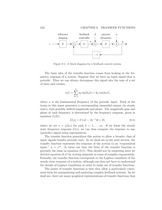
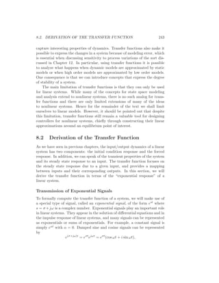
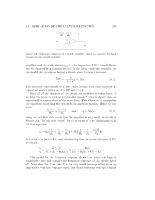
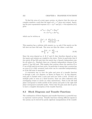
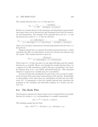
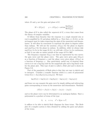
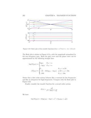
278. 266 CHAPTER 8. TRANSFER FUNCTIONS
10
2
10
3
10
4
10
0
10
1
10
2
10
3
10
4
−270
−180
−90
0
GainPhase
Frequency [Hz]
Figure 8.13: Frequency response of a piezoelectric drive for an atomic force micro-
scope. The input is the voltage to the drive amplifier and the output is the output
of the amplifier that measures beam deflection.
introduced in Section 3.5. Experimental determination of the frequency re-
sponse is particularly attractive for this system because its dynamics are
very fast and hence experiments can be done quickly. A typical example is
given in Figure 8.13, which shows an experimentally determined frequency
response (solid line). In this case the frequency response was obtained in
less than a second. The transfer function
G(s) =
kω2
2ω2
3ω2
5(s2 + 2ζ1ω1s + ω2
1)(s2 + 2ζ4ω4s + ω2
4)e−sT
ω2
1ω2
4(s2 + 2ζ2ω2s + ω2
2)(s2 + 2ζ3ω3s + ω2
3)(s2 + 2ζ5ω5s + ω2
5)
with ω1 = 2420, ζ1 = 0.03, ω2 = 2550, ζ2 = 0.03, ω3 = 6450, ζ3 = 0.042,
ω4 = 8250, ζ4 = 0.025, ω5 = 9300, ζ5 = 0.032, T = 10−4, and k = 5. was
fit to the data (dashed line). The frequencies associated with the zeros are
located where the gain curve has minima and the frequencies associated with
the poles are located where the gain curve has local maxima. The relative
damping are adjusted to give a good fit to maxima and minima. When a
good fit to the gain curve is obtained the time delay is adjusted to give a
good fit to the phase curve. ∇
Experimental determination of frequency response is less attractive for
systems with slow dynamics because the experiment takes a long time.
Example 8.7 (Pupillary light reflex dynamics). The human eye is an organ
that is easily accessible for experiments. It has a control system that adjusts

279. 8.5. TRANSFER FUNCTIONS FROM EXPERIMENTS 267
Figure 8.14: Light stimulation of the eye. In A the light beam is so large that
it always covers the whole pupil, giving the closed loop dynamics. In B the light
is focused into a beam which is so narrow that it is not influenced by the pupil
opening, giving the open loop dynamics. In C the light beam is focused on the
edge of the pupil opening, which has the effect of increasing the gain of the system
since small changes in the pupil opening have a large effect on the amount of light
entering the eye. From [Sta59].
the pupil opening to regulate the light intensity at the retina. This control
system was explored extensively by Stark in the late 1960s [Sta68]. To de-
termine the dynamics, light intensity on the eye was varied sinusoidally and
the pupil opening was measured. A fundamental difficulty is that the closed
loop system is insensitive to internal system parameters, so analysis of a
closed loop system thus gives little information about the internal proper-
ties of the system. Stark used a clever experimental technique that allowed
him to investigate both open and closed loop dynamics. He excited the
system by varying the intensity of a light beam focused on the eye and he
measured pupil area; see Figure 8.14. By using a wide light beam that covers
the whole pupil the measurement gives the closed loop dynamics. The open
loop dynamics were obtained by using a narrow beam, which is small enough
that it is not influenced by the pupil opening. The result of one experiment
for determining open loop dynamics is given in Figure 8.15. Fitting a trans-
fer function to the gain curves gives a good fit for G(s) = 0.17/(1 + 0.08s)3.
This curve gives a poor fit to the phase curve as shown by the dashed curve
in Figure 8.15. The fit to the phase curve is improved by adding a time
delay, which leaves the gain curve unchanged while substantially modifying
the phase curve. The final fit gives the model
G(s) =
0.17
(1 + 0.08)3
e−0.2s
.
The Bode plot of this is shown with dashed curves in Figure 8.15. ∇
Notice that for both the AFM drive and the pupillary dynamics it is
not easy to derive appropriate models from first principles. In practice, it is

280. 268 CHAPTER 8. TRANSFER FUNCTIONS
2 5 10 20
0.01
0.02
0.05
0.1
0.2
2 5 10 20
−360
−180
0
ω
|G(jω)|∠G(jω)
Figure 8.15: Sample curves from open loop frequency response of the eye (left) and
Bode plot for the open loop dynamics (right). Redrawn from the data of [Sta59].
The dashed curve in the Bode plot is the minimum phase curve corresponding to
the gain curve.
often fruitful to use a combination of analytical modeling and experimental
identification of parameters.
8.6 Laplace Transforms
Transfer functions are typically introduced using Laplace transforms and in
this section we derive the transfer function using this formalism. We assume
basic familiarity with Laplace transforms; students who are not familiar with
them can safely skip this section.
Traditionally, Laplace transforms were also used to compute responses
of linear system to different stimuli. Today we can easily generate the re-
sponses using computers. Only a few elementary properties are needed for
basic control applications. There is, however, a beautiful theory for Laplace
transforms that makes it possible to use many powerful tools of the theory
of functions of a complex variable to get deep insights into the behavior of
systems.
Definitions and Properties
Consider a time function f : R+ → R which is integrable and grows no faster
than es0t for some finite s0 ∈ R and large t. The Laplace transform maps f

281. 8.6. LAPLACE TRANSFORMS 269
to a function F = Lf : C → C of a complex variable. It is defined by
F(s) =
∞
0
e−st
f(t) dt, Re s > s0. (8.20)
The transform has some properties that makes it very well suited to deal
with linear systems.
First we observe that the transform is linear because
L(af + bg) =
∞
0
e−st
(af(t) + bg(t)) dt
= a
∞
0
e−st
f(t) dt + b
∞
0
e−st
g(t) dt = aLf + bLg.
(8.21)
Next we will calculate the Laplace transform of the derivative of a function.
We have
L
df
dt
=
∞
0
e−st
f′
(t) dt = e−st
f(t)
∞
0
+ s
∞
0
e−st
f(t) dt = −f(0) + sLf,
where the second equality is obtained by integration by parts. We thus
obtain the following important formula for the transform of a derivative
L
df
dt
= sLf − f(0) = sF(s) − f(0). (8.22)
This formula is particularly simple if the initial conditions are zero because
it follows that differentiation of a function corresponds to multiplication of
the transform with s.
Since differentiation corresponds to multiplication with s we can expect
that integration corresponds to division by s. This is true, as can be seen
by calculating the Laplace transform of an integral. We have
L
t
0
f(τ) dτ =
∞
0
e−st
t
0
f(τ) dτ dt
= −
e−st
s
t
0
e−sτ
f(τ) dτ
∞
0
+
∞
0
e−sτ
s
f(τ) dτ =
1
s
∞
0
e−sτ
f(τ) dτ,
hence
L
t
0
f(τ) dτ =
1
s
Lf =
1
s
F(s). (8.23)
Integration of a time function thus corresponds to dividing the Laplace trans-
form by s.

282. 270 CHAPTER 8. TRANSFER FUNCTIONS
The Laplace Transform of a Convolution
Consider a linear time-invariant system with zero initial state. The relation
between the input u and the output y is given by the convolution integral
y(t) =
∞
0
h(t − τ)u(τ) dτ,
where h(t) is the impulse response for the system. We will now consider the
Laplace transform of such an expression. We have
Y (s) =
∞
0
e−st
y(t) dt =
∞
0
e−st
∞
0
h(t − τ)u(τ) dτ dt
=
∞
0
t
0
e−s(t−τ)
e−sτ
h(t − τ)u(τ) dτ dt
=
∞
0
e−sτ
u(τ) dτ
∞
0
e−st
h(t) dt = H(s)U(s)
The result can be written as Y (s) = H(s)U(s) where H, U and Y are the
Laplace transforms of h, u and y. The system theoretic interpretation is
that the Laplace transform of the output of a linear system is a product
of two terms, the Laplace transform of the input U(s) and the Laplace
transform of the impulse response of the system H(s). A mathematical
interpretation is that the Laplace transform of a convolution is the product
of the transforms of the functions that are convolved. The fact that the
formula Y (s) = H(s)U(s) is much simpler than a convolution is one reason
why Laplace transforms have become popular in control.
The Transfer Function
The properties (8.21) and (8.22) makes the Laplace transform ideally suited
for dealing with linear differential equations. The relations are particularly
simple if all initial conditions are zero.
Consider for example a linear state space system described by
˙x = Ax + Bu
y = Cx + Du.
Taking Laplace transforms under the assumption that all initial values are
zero gives
sX(s) = AX(s) + BU(s)
Y (s) = CX(s) + DU(s).

283. 8.7. FURTHER READING 271
Elimination of X(s) gives
Y (s) = C(sI − A)−1
B + D U(s). (8.24)
The transfer function is thus G(s) = C(sI − A)−1B + D (compare with
equation (8.4)).
The formula (8.24) has a strong intuitive interpretation because it tells
that the Laplace transform of the output is the product of the transfer
function of the system and the transform of the input. In the transform
domain the action of a linear system on the input is simply a multiplication
with the transfer function. The transfer function is a natural generalization
of the concept of gain of a system.
8.7 Further Reading
Heaviside, who introduced the idea to characterize dynamics by the response
to a unit step function, also introduced a formal operator calculus for an-
alyzing linear systems. This was a significant advance because it gave
the possibility to analyze linear systems algebraically. Unfortunately it was
difficult to formalize Heaviside’s calculus properly. This was not done until
the the mathematician Laurent Schwartz developed the distribution the-
ory in the late 1940s. Schwartz was given the Fields Medal in 1950. The
idea of characterizing a linear system by its steady state response to sinu-
soids was introduced by Fourier in his investigation of heat conduction in
solids [Fou07]. Much later it was used by Steinmetz when he introduced the
jω method to develop a theory for alternating currents.
The concept of transfer functions was an important part of classical con-
trol theory; see [JNP47]. It was introduced via the Laplace transform by
Gardner Barnes [GB42], who also used it to calculate response of linear
systems. The Laplace transform was very important in the early phase of
control because it made it possible to find transients via tables. The Laplace
transform is of less importance today when responses to linear systems can
easily be generated using computers. For a mathematically inclined audi-
ence it is still a very convenient to introduce the transfer function via the
Laplace transform, which is an important part of applied mathematics. For
an audience with less background in mathematics it may be preferable to
introduce the transfer function via the particular solution generated by the
input est as was done in Section 8.2.
There are many excellent books on the use of Laplace transforms and
transfer functions for modeling and analysis of linear input/output systems.

284. 272 CHAPTER 8. TRANSFER FUNCTIONS
Traditional texts on control, such as [FPEN05] and [DB04], are representa-
tive examples.
8.8 Exercises
1. Let G(s) be the transfer function for a linear system. Show that if we
apply an input u(t) = A sin(ωt) then the steady state output is given
by y(t) = |G(jω)|A sin(ωt + arg G(jω)).
2. Show that the transfer function of a system only depends on the dy-
namics in the reachable and observable subspace of the Kalman de-
composition.
3. The linearized model of the pendulum in the upright position is char-
acterized by the matrices
A =


0 1
1 0

 , B =


0
1

 , C =

1 0

 , D = 0.
Determine the transfer function of the system.
4. Compute the frequency response of a PI controller using an op amp
with frequency response given by equation (8.12).
5. Consider the speed control system given in Example 6.9. Compute
the transfer function between the throttle position u, angle of the
road θ and the speed of the vehicle v assuming a nominal speed ve
with corresponding throttle position ue.
6. Consider the differential equation
dny
dtn
+ a1
dn−1y
dtn−1
+ a2
dn−2y
dtn−2
+ · · · + any = 0
Let λ be a root of the polynomial
sn
+ a1sn−1
+ · · · + an = 0.
Show that the differential equation has the solution y(t) = eλt.
7. Consider the system
dny
dtn
+ a1
dn−1y
dtn−1
+ · · · + any = b1
dn−1u
dtn−1
+ b2
dn−2u
dtn−2
+ · · · + bnu,

285. 8.8. EXERCISES 273
(a) (b)
Figure 8.16: Schematic diagram of the quarter car model (a) and of a vibration
absorber right (b).
Let λ be a zero of the polynomial
b(s) = b1sn−1
+ b2sn−2
+ · · · + bn
Show that if the input is u(t) = eλt then there is a solution to the
differential equation that is identically zero.
8. Active and passive damping is used in cars to give a smooth ride on
a bumpy road. A schematic diagram of a car with a damping system
in shown in Figure 8.16(a). The car is approximated with two masses,
one represents a quarter of the car body and the other a wheel. The
actuator exerts a force F between the wheel and the body based on
feedback from the distance between body and the center of the wheel
(the rattle space). A simple model of the system is given by Newton’s
equations for body and wheel
mb¨xb = F, mw ¨xw = −F + kt(xr − xw),
where mb is a quarter of the body mass, mw is the effective mass
of the wheel including brakes and part of the suspension system (the
unsprung mass), and kt is the tire stiffness. Furthermore xb, xw and xr
represent the heights of body, wheel, and road, measured from their
equilibria. For a conventional damper consisting of a spring and a

286. 274 CHAPTER 8. TRANSFER FUNCTIONS
damper we have F = k(xw − xb) + c( ˙xw − ˙xb), for an active damper
the force F can be more general and it can also depend on riding
conditions. Rider comfort can be characterized by the transfer function
Gaxr from road height xr to body acceleration a = ¨xb. Show that this
transfer function has the property Gaxr (iωt) = kt/mb, where ωt =
kt/mw (the tire hop frequency). The equation implies that there are
fundamental limitations to the comfort that can be achieved with any
damper. More details are given in [HB90].
9. Damping vibrations is a common engineering problem. A schematic
diagram of a damper is shown in Figure 8.16(b). The disturbing vibra-
tion is a sinusoidal force acting on mass m1 and the damper consists
of mass m2 and the spring k2. Show that the transfer function from
disturbance force to height x1 of the mass m1 is
Gx1F =
m2s2 + k2
m1m2s4 + m2c1s3 + (m1k2 + m2(k1 + k2))s2 + k2c1s + k1k2
How should the mass m2 and the stiffness k2 be chosen to eliminate
a sinusoidal oscillation with frequency ω0. More details are given on
pages 87–93 in the classic text on vibrations [DH85].
10. Consider the linear state space system
˙x = Ax + Bu
y = Cx.
Show that the transfer function is
G(s) =
b1sn−1 + b2sn−2 + · · · + bn
sn + a1sn−1 + · · · + an
where
b1 = CB
b2 = CAB + a1CB
b3 = CA2
B + a1CAB + a2CB
...
bn = CAn−1
B + a1CAn−1
B + · · · + an−1CB
and λ(s) = sn + a1sn−1 + · · · + an is the characteristic polynomial for
A.

287. 8.8. EXERCISES 275
11. Consider a closed loop system of the form of Figure 8.6 with F = 1 and
P and C having a common pole. Show that if each system is written
in state space form, the resulting closed loop system is not reachable
and not observable.
12. The Physicist ˚Angstr¨om, who is associated with the length unit ˚A,
used frequency response to determine thermal diffusivity of metals [˚Ang61].
Heat propagation in a metal rod is described by the partial differential
equation
∂T
∂t
= a
∂2T
∂x2
− µT, (8.25)
where a = λ
ρC is the thermal diffusivity, and the last term represents
thermal loss to the environment. Show that the transfer function re-
lating temperatures at points with the distance ℓ is
G(s) = e−ℓ
√
(s+µ)/a
, (8.26)
and the frequency response is given by
log |G(iω)| = −ℓ
µ + ω2 + µ2
2a
arg G(iω) = −ℓ
−µ + ω2 + µ2
2a
.
Also derive the following equation
log |G(iω)| arg G(iω) =
ℓ2ω
2a
.
This remarkably simple formula shows that diffusivity can be deter-
mined from the value of the transfer function at one frequency. It was
the key in ˚Angstr¨om’s method for determining thermal diffusivity. No-
tice that the parameter µ which represents the thermal losses does not
appear in the formula.

288. 276 CHAPTER 8. TRANSFER FUNCTIONS

289. Chapter 9
Loop Analysis
Regeneration or feed-back is of considerable importance in many applications
of vacuum tubes. The most obvious example is that of vacuum tube oscil-
lators, where the feed-back is carried beyond the singing point. Another ap-
plication is the 21-circuit test of balance, in which the current due to the
unbalance between two impedances is fed back, the gain being increased until
singing occurs. Still other applications are cases where portions of the output
current of amplifiers are fed back to the input either unintentionally or by de-
sign. For the purpose of investigating the stability of such devices they may
be looked on as amplifiers whose output is connected to the input through a
transducer. This paper deals with the theory of stability of such systems.
Abstract for “Regeneration Theory”, Harry Nyquist, 1932 [Nyq32].
In this chapter we study how how stability and robustness of closed loop
systems can be determined by investigating how signals propagate around
the feedback loop. The Nyquist stability theorem is a key result that pro-
vides a way to analyze stability and introduce measures of degrees of stabil-
ity.
9.1 The Loop Transfer Function
The basic idea of loop analysis is to trace how a sinusoidal signal propagates
in the feedback loop and explore the resulting stability by investigating if
the signal grows or decays around the loop. This is easy to do because the
transmission of sinusoidal signals through a (linear) dynamical system is
characterized by the frequency response of the system. The key result is the
Nyquist stability theorem, which provides a great deal of insight regarding
the stability of a system. Unlike proving stability with Lyapunov functions,
277

290. 278 CHAPTER 9. LOOP ANALYSIS
C(s) P(s)Σ
r y
−1
AB
−1
L(s)
(a) (b)
Figure 9.1: Block diagram of a (a) simple feedback system with (b) the loop opened
at AB.
studied in Chapter 4, the Nyquist criterion allows us to determine more than
just whether a system is stable or unstable. It provides a measure of the
degree of stability through the definition of stability margins. The Nyquist
theorem also indicates how an unstable system should be changed to make
it stable, which we shall study in detail in Chapters 10–12.
Consider the system in Figure 9.1a. The traditional way to determine
if the closed loop system is stable is to investigate if the closed loop char-
acteristic polynomial has all its roots in the left half plane. If the process
and the controller have rational transfer functions P(s) = np(s)/dp(s) and
C(s) = nc(s)/dc(s), then the closed loop system has the transfer function
Gyr =
PC
1 + PC
=
np(s)nc(s)
dp(s)dc(s) + np(s)nc(s)
,
and the characteristic polynomial is
λ(s) = dp(s)dc(s) + np(s)nc(s).
To check stability, we simply compute the roots of the characteristic poly-
nomial and verify that they all have negative real part. This approach is
straightforward but it gives little guidance for design: it is not easy to tell
how the controller should be modified to make an unstable system stable.
Nyquist’s idea was to investigate conditions under which oscillations can
occur in a feedback loop. To study this, we introduce the loop transfer
function,
L = PC,
which is the transfer function obtained by breaking the feedback loop, as
shown in Figure 9.1. The loop transfer function is simply the transfer func-
tion from the input at position A to the output at position B.

291. 9.2. THE NYQUIST CRITERION 279
We will first determine conditions for having a periodic oscillation in
the loop. Assume that a sinusoid of frequency ω0 is injected at point A. In
steady state the signal at point B will also be a sinusoid with the frequency
ω0. It seems reasonable that an oscillation can be maintained if the signal
at B has the same amplitude and phase as the injected signal, because we
could then connect A to B. Tracing signals around the loop we find that the
signals at A and B are identical if
L(jω0) = −1, (9.1)
which provides a condition for maintaining an oscillation. The key idea of
the Nyquist stability criterion is to understand when this can happen in a
very general setting. As we shall see, this basic argument becomes more
subtle when the loop transfer function has poles in the right half plane.
One of the powerful concepts embedded in Nyquist’s approach to sta-
bility analysis is that it allows us to determine the stability of the feedback
system by looking at properties of the open loop transfer function. This idea
will turn out to be very important in how we approach designing transfer
functions.
9.2 The Nyquist Criterion
In this section we present Nyquist’s criterion for determining the stability of
a feedback system through analysis of the loop transfer function. We begin
by introducing a convenient graphical tool, the Nyquist plot, and showing
how it can be used to ascertain stability.
The Nyquist Plot
The frequency response of the loop transfer function can be represented by
plotting the complex number L(jω) as a function of ω. Such a plot is called
a Nyquist plot and the curve is called a Nyquist curve. An example of a
Nyquist plot is given in Figure 9.2. The magnitude |L(jω)| is called the
loop gain because it tells how much the signal is amplified as is passes around
the feedback loop.
The condition for oscillation given in equation (9.1) implies that the
Nyquist curve of the loop transfer function goes through the point L = −1,
which is called the critical point. Intuitively it seems reasonable that the
system is stable if |L(jωc)| < 1, which means that the critical point −1
is on the left hand side of the Nyquist curve, as indicated in Figure 9.2.

292. 280 CHAPTER 9. LOOP ANALYSIS
Re L(jω)Re L(jω)Re L(jω)
Im L(jω)Im L(jω)Im L(jω)
ωωω
arg L(jω)arg L(jω)arg L(jω)
|L(jω)||L(jω)||L(jω)|
−1−1−1
Figure 9.2: Nyquist plot of the transfer function L(s) = 1.4e−s
/(s + 1)2
. The gain
and phase at the frequency ω are g = |L(jω)| and ϕ = arg L(jω).
This means that the signal at point B will have smaller amplitude than the
injected signal. This is essentially true, but there are several subtleties that
requires a proper mathematical analysis to clear up, and which we defer
until the next section. For now we consider a simplified case, when the loop
transfer function is stable.
For loop transfer functions that do not have poles in the right half plane,
the precise stability condition is that the complete Nyquist plot does not en-
circle the critical point −1. The complete Nyquist plot is obtained by adding
the plot for negative frequencies shown in the dashed curve in Figure 9.2.
This plot is the mirror image of the Nyquist curve about the real axis.
Theorem 9.1 (Simplified Nyquist criterion). Let L(s) be the loop transfer
function for a negative feedback system (as shown in Figure 9.1) and assume
that L has no poles in the closed right half plane (Re s ≥ 0). Then the closed
loop system is stable if and only if the closed contour given by Ω = {L(jω) :
−∞ < ω < ∞} ⊂ C has no net encirclements of s = −1.
The following conceptual procedure can be used to determine that there
are no encirclements: Fix a pin at the critical point s = −1 orthogonal to
the plane. Attach a string with one end at the critical point and the other
to the Nyquist plot. Let the end of the string attached to the Nyquist curve
traverse the whole curve. There are no encirclements if the cord does not

293. 9.2. THE NYQUIST CRITERION 281
wind up on the pin when the curve is encircled.
Example 9.1 (Cruise control). Consider the speed control system intro-
duced in Section 3.1 and analyzed using state space techniques in Exam-
ple 6.9. In this example, we study the stability of the system using the
Nyquist criterion.
The linearized dynamics around the equilibrium speed ve and throttle
position ue are given by
˙˜v = a˜v − gθ + b˜u
y = v = ˜v + ve,
where ˜v = v − ve, ˜u = u − ue, m is the mass of the car and θ is the angle of
the road. The constant a < 0 depends on the throttle characteristic and is
given in Example 5.10.
The transfer function from throttle to speed is given by
P(s) = Gyu(s) =
b
s − α
.
We consider a controller that is a modified version of the proportional-
integral (PI) controller given previously. Assume that the transfer function
of the controller is
C(s) = Gue(s) = kp +
ki
s + β
=
kps + ki + kpβ
s + β
giving a loop transfer function of
L(s) = b
kps + ki + kpβ
(s + a)(s + β)
.
The Nyquist plot for the system, using a = 0.0101, b = 1.3203, kp = 0.5,
ki = 0.1 and β = 0.1, is shown in Figure 9.3. We see from the Nyquist plot
that the closed loop system is stable, since there are no net encirclements of
the -1 point. ∇
One nice property of the Nyquist stability criterion is that it can be applied
to infinite dimensional systems, as is illustrated by the following example.
Example 9.2 (Heat conduction). Consider a temperature control system
where the heat conduction process has the transfer function
P(s) = e−
√
s

294. 282 CHAPTER 9. LOOP ANALYSIS
−5 0 5 10 15
−10
−8
−6
−4
−2
0
2
4
6
8
10
Re
Im
Figure 9.3: Nyquist plot for the speed control system.
and the controller is a proportional controller with gain k. The loop transfer
function is L(s) = ke−
√
s and its Nyquist plot for k = 1 is shown in Fig-
ure 9.4. To compute the stability condition for the system as a function of
the gain k, we analyze the transfer function a bit more carefully. We have
P(jω) = e−
√
jω
= e−
√
ω/2−i
√
ω/2
and hence
log P(jω) = − jω = −
ω
√
2
2
− i
ω
√
2
2
and
arg L(jω) = −
ω
√
2
2
.
The phase is −π for ω = ωc = π/
√
2 and the gain at that frequency is
ke−π ≈ 0.0432k. The Nyquist plot for a system with gain k is obtained
simply by multiplying the Nyquist curve in the figure by k. The Nyquist
curve reaches the critical point L = −1 for k = eπ = 23.1. The complete
Nyquist curve in Figure 9.4 shows that the Nyquist curve does not encircle
the critical point if k < eπ, giving a stability condition for the system. ∇

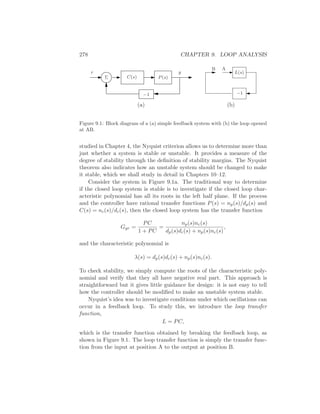
295. 9.2. THE NYQUIST CRITERION 283
Re L(jω)
Im L(jω)
1
Figure 9.4: Nyquist plot of the transfer function L(s) = e−
√
s
Nyquist’s Stability Theorem
We will now state and prove the Nyquist stability theorem for a general loop
transfer function L(s). This requires some results from the theory of complex
variables, for which the reader can consult [?] and the references therein.
Since some precision is needed in stating Nyquist’s criterion properly, we
will also use a more mathematical style of presentation. The key result is
the following theorem about functions of complex variables.
Theorem 9.2 (Principle of variation of the argument). Let D be a closed
region in the complex plane and let Γ be the boundary of the region. Assume
the function f : C → C is analytic in D and on Γ, except at a finite number
of poles and zeros. Then the winding number, wn, is given by
wn =
1
2π
∆Γ arg f(z) =
1
2πi Γ
f′(z)
f(z)
dz = N − P,
where ∆Γ is the net variation in the angle along the contour Γ, N is the
number of zeros and P the number of poles in D. Poles and zeros of multi-
plicity m are counted m times.
Proof. Assume that z = a is a zero of multiplicity m. In the neighborhood
of z = a we have
f(z) = (z − a)m
g(z),

296. 284 CHAPTER 9. LOOP ANALYSIS
where the function g is analytic and different from zero. The ratio of the
derivative of f to itself is then given by
f′(z)
f(z)
=
m
z − a
+
g′(z)
g(z)
and the second term is analytic at z = a. The function f′/f thus has a
single pole at z = a with the residue m. The sum of the residues at the
zeros of the function is N. Similarly we find that the sum of the residues of
the poles of is −P. Furthermore we have
d
dz
log f(z) =
f′(z)
f(z)
,
which implies that
Γ
f′(z)
f(z)
dz = ∆Γ log f(z),
where ∆Γ again denotes the variation along the contour Γ. We have
log f(z) = log |f(z)| + i arg f(z).
Since the variation of |f(z)| around a closed contour is zero we have
∆Γ log f(z) = i∆Γ arg f(z)
and the theorem is proven.
This theorem is useful for determining the number of poles and zeros of a
function of complex variables in a given region. By choosing an appropriate
closed region D with boundary Γ, we can determine the difference between
the number of poles and zeros through computation of the winding number.
Theorem 9.2 can be used to prove Nyquist’s stability theorem by choos-
ing Γ as the Nyquist contour shown in Figure 9.5, which encloses the right
half plane. To construct the contour, we start with part of the imaginary
axis −iR ≤ s ≤ iR, and a semicircle to the right with radius R. If the
function f has poles on the imaginary axis we introduce small semicircles
with radii r to the right of the poles as shown in the figure. The Nyquist
contour is obtained by letting R → ∞ and r → 0. We call the contour Γ
the full Nyquist contour, sometimes call the “D contour”.
To see how we used this to compute stability, consider a closed loop
system with the loop transfer function L(s). The closed loop poles of the
system are the zeros of the function
f(s) = 1 + L(s).

297. 9.2. THE NYQUIST CRITERION 285
R
Γ
r
r
r
Figure 9.5: The Nyquist contour Γ.
To find the number of zeros in the right half plane, we investigate the winding
number of the function f(s) = 1 + L(s) as s moves along the Nyquist con-
tour Γ in the clockwise direction. The winding number can conveniently be
determined from the Nyquist plot. A direct application of the Theorem 9.2
gives the following result.
Theorem 9.3 (Nyquist’s stability theorem). Consider a closed loop system
with the loop transfer function L(s), which which has P poles in the region
enclosed by the Nyquist contour. Let wn be the winding number of the func-
tion f(s) = 1 + L(s) when s encircles the Nyquist contour Γ. The closed
loop system then has wn + P poles in the right half plane.
Since the image of 1+L(s) is simply a shifted version of L(s), we usually
restate the Nyquist criterion as net encirclements of the −1 point by the
image of L(s).
There is a subtlety with the Nyquist plot when the loop transfer function
has poles on the imaginary axis because the gain is infinite at the poles. This
means that the map of the small semicircles are infinitely large half circles.
When plotting Nyquist curves on the computer, one must be careful to see
that the such poles are properly handled and often one must sketch those
portions of the Nyquist plot by hand, being careful to loop the right way
around the poles.
We illustrate Nyquist’s theorem by a series of examples.

298. 286 CHAPTER 9. LOOP ANALYSIS
Re L(jω)
Im L(jω)
Figure 9.6: The complete Nyquist curve for the loop transfer function L(s) =
k
s(s+1)2 . The curve is drawn for k < 2. The map of the positive imaginary axis
is shown in full lines, the map of the negative imaginary axis and the small semi
circle at the origin in dashed lines.
Example 9.3. Consider a closed loop system with the loop transfer function
L(s) =
k
s(s + 1)2
.
Figure 9.6 shows the image of the contour Γ under the map L. The loop
transfer function does not have any poles in the region enclosed by the
Nyquist contour. By computing the phase of L, one can show that the
Nyquist plot intersects the imaginary axis for ω = 1 and the intersection is
at −k/2. It follows from Figure 9.6 that the winding number is zero if k < 2
and 2 if k > 2. We can thus conclude that the closed loop system is stable if
k < 2 and that the closed loop system has two roots in the right half plane
if k > 2. ∇
Next we will consider a case where the loop transfer function has a pole
inside the Nyquist contour.
Example 9.4 (Loop transfer function with RHP pole). Consider a feedback
system with the loop transfer function
L(s) =
k
s(s − 1)(s + 5)
.

299. 9.2. THE NYQUIST CRITERION 287
Re L(jω)
Im L(jω)
Figure 9.7: Complete Nyquist plot for the loop transfer function L(s) = k
s(s−1)(s+5) .
The map of the positive imaginary axis is shown in full lines, the map of the negative
imaginary axis and the small semi circle at the origin in dashed lines.
This transfer function has a pole at s = 1 which is inside the Nyquist
contour. The complete Nyquist plot of the loop transfer function is shown in
Figure 9.7. Traversing the contour Γ in clockwise we find that the winding
number is wn = 1. It follows from the principle of the variation of the
argument that the closed loop system has wn +P = 2 poles in the right half
plane and hence is unstable. ∇
Normally, we find that unstable systems can be stabilized simply by re-
ducing the loop gain. There are however situations where a system can be
stabilized by increasing the gain. This was first encountered by electrical
engineers in the design of feedback amplifiers who coined the term condi-
tional stability. The problem was actually a strong motivation for Nyquist
to develop his theory. We will illustrate by an example.
Example 9.5 (Conditional stability). Consider a feedback system with the
loop transfer function
L(s) =
3(s + 1)2
s(s + 6)2
. (9.2)
The Nyquist plot of the loop transfer function is shown in Figure 9.8. Notice
that the Nyquist curve intersects the negative real axis twice. The first
intersection occurs at L = −12 for ω = 2 and the second at L = −4.5 for
ω = 3. The intuitive argument based on signal tracing around the loop in
Figure 9.1 is strongly misleading in this case. Injection of a sinusoid with
frequency 2 rad/s and amplitude 1 at A gives, in steady state, an oscillation

300. 288 CHAPTER 9. LOOP ANALYSIS
Re L(jω)
Im L(jω)
−1
Re L(jω)
Im L(jω)
Figure 9.8: Nyquist curve for the loop transfer function L(s) = 3(s+1)2
s(s+6)2 . The plot
on the right is an enlargement of the area around the origin of the plot on the left.
at B that is in phase with the input and has amplitude 12. Intuitively it
is seems unlikely that closing of the loop will result a stable system. It
follows from Nyquist’s stability criterion that the system is stable because
the critical point is to the left of the Nyquist curve when it is traversed for
increasing frequencies. ∇
9.3 Stability Margins
In practice it is not enough that a system is stable. There must also be some
margins of stability that describe how stable the system is and its robustness
to perturbations. There are many ways to express this, but one of the most
common is the use of gain and phase margins, inspired by Nyquist’s stability
criterion. The key idea is that it is easy to plot of the loop transfer function
L(s). An increase of controller gain simply expands the Nyquist plot radially.
An increase of the phase of the controller twists the Nyquist plot clockwise.
Hence from the Nyquist plot we can easily pick off the amount of gain or
phase that can be added without causing the system to go unstable.
Let ω180 be the phase crossover frequency, which is the smallest frequency
where the phase of the loop transfer function L(s) is −180◦. The gain margin
is defined as
gm =
1
|L(jω180)|
. (9.3)
It tells how much the controller gain can be increased before reaching the
stability limit.

301. 9.3. STABILITY MARGINS 289
Re L(jω)
Im L(jω)
−1
ϕm
sm
−1/gm
Figure 9.9: Nyquist plot of the loop transfer function L with gain margin gm, phase
margin ϕm and stability margin sm.
Similarly, let ωgc be the gain crossover frequency, the lowest frequency
where the loop transfer function L(s) has unit magnitude. The phase margin
is
ϕm = π + arg L(jωgc), (9.4)
the amount of phase lag required to reach the stability limit. The margins
have simple geometric interpretations in the Nyquist diagram of the loop
transfer function as is shown in Figure 9.9.
A drawback with gain and phase margins is that it is necessary to give
both of them in order to guarantee that the Nyquist curve not is close to the
critical point. An alternative way to express margins is by a single number,
the stability margin, sm, which is the shortest distance from the Nyquist
curve to the critical point. This number also has other nice interpretations
as will be discussed in Chapter 12.
When we are designing feedback systems, it will often be useful to define
the robustness of the system using gain, phase and stability margins. These
numbers tell us how much the system can vary from our nominal model
and still be stable. Reasonable values of the margins are phase margin
ϕm = 30◦−60◦, gain margin gm = 2−5, and stability margin sm = 0.5−0.8.
There are also other stability measures, such as the delay margin, which
is the smallest time delay required to make the system unstable. For loop
transfer functions that decay quickly the delay margin is closely related to

302. 290 CHAPTER 9. LOOP ANALYSIS
10
−1
10
0
10
−1
10
0
10
1
10
−1
10
0
−180
−150
−120
−90
|L(jω)|∠L(jω)
ω
log10 gm
ϕm
Figure 9.10: Finding gain and phase margins from the Bode plot of the loop transfer
function. The loop transfer function is L(s) = 1/(s(s + 1)(s + 2)), the gain margin
is gm = 6.0, the gain crossover frequency ωgc = 1.42., the phase margin is ϕm = 53◦
at the phase crossover frequency ω = 0.44.
the phase margin but for systems where the amplitude ratio of the loop
transfer function has several peaks at high frequencies the delay margin is a
more relevant measure. A more detailed discussion of robustness measures
is given in Chapter 12.
Gain and phase margins can also be determined from the Bode plot of
the loop transfer function. A change of controller gain translates the gain
curve vertically and it has no effect on the phase curve. To determine the
gain margin we first find the phase crossover frequency ω180 where the phase
is −180◦. The gain margin is the inverse of the gain at that frequency. To
determine the phase margin we first determine the gain crossover frequency
ωgc, i.e. the frequency where the gain of the loop transfer function is one.
The phase margin is the phase of the loop transfer function at that frequency
plus 180◦. Figure 9.10 illustrates how the margins are found in the Bode
plot of the loop transfer function. The stability margin cannot easily be
found from the Bode plot of the loop transfer function. There are however
other Bode plots that will give sm; these will be discussed in Chapter 12.
Example 9.6 (Vehicle steering). Consider the linearized model for vehicle
steering with a controller based on state feedback. The transfer function of

303. 9.3. STABILITY MARGINS 291
−1.5 −1 −0.5 0 0.5
−1.5
−1
−0.5
0
0.5
ReL(jω)
ImL(jω)
10
−1
10
0
10
1
10
−2
10
−1
10
0
10
1
10
2
10
−1
10
0
10
1
−180
−170
−160
−150
−140
−130
|L(jω)|∠L(jω)
ω
Figure 9.11: Nyquist (left) and Bode (right) plots of the loop transfer function for
vehicle steering with a controller based on state feedback and an observer.
the process is
P =
αs + 1
s2
.
and the controller has the transfer function
C =
s(k1l1 + k2l2) + k1l2
s2 + s(αk1 + k2 + l1) + k1 + l2 + k2l1 − αk2l2
,
as computed in Example 8.4. The Nyquist and Bode plots of the loop
transfer function L = PC for the process parameter a = 0.5, and a controller
characterized by ωc = 1, ζc = 0.707, ωo = 2, ζo = 0.707 are shown in
Figure 9.11. The gains of the state feedback are k1 = 1 and k2 = 0.914,
and the observer gains are l1 = 2.828 and l2 = 4. The phase margin of the
system is 44◦ and the gain margin is infinite since the phase lag is never
greater than 180◦, indicating that the closed loop system is robust. ∇
Example 9.7 (Pupillary light reflex dynamics). The pupillary light reflex
dynamics was discussed in Example 8.7. Stark found a clever way to
artificially increase the loop gain by focusing a narrow beam at the boundary
of the pupil. It was possible to increase the gain so much that the pupil
started to oscillate. The Bode plot in Figure 9.12b shows that the phase
crossover frequency is ωgc = 8 rad/s. This is in good agreement with Stark’s
experimental investigations which gave an average frequency of 1.35 Hz or
8.5 rad/s. ∇

304. 292 CHAPTER 9. LOOP ANALYSIS
2 5 10 20
0.01
0.02
0.05
0.1
0.2
2 5 10 20
−360
−180
0
ω
|G(jω)|∠G(jω)
Figure 9.12: Sample curves from open loop frequency response of the eye (left)
and Bode plot for the open loop dynamics (right). See Example 8.7 for a detailed
description.
9.4 Bode’s Relations
An analysis of Bode plots reveals that there appears to be be a relation
between the gain curve and the phase curve. Consider for example the Bode
plots for the differentiator and the integrator (shown in Figure 8.10). For
the differentiator the slope is +1 and the phase is constant π/2 radians.
For the integrator the slope is −1 and the phase is −π/2. For the first
order system G(s) = s + a, the amplitude curve has the slope 0 for small
frequencies and the slope +1 for high frequencies and the phase is 0 for low
frequencies and π/2 for high frequencies.
Bode investigated the relations between the curves for systems with no
poles and zeros in the right half plane. He found that the phase was a
uniquely given by the gain and vice versa:
arg G(jω0) =
1
π
∞
0
d log |G(jω)|
d log ω
log
ω + ω0
ω − ω0
d log ω
π
2
∞
0
f(ω)
d log |G(jω)|
d log ω
d log ω ≈
π
2
d log |G(jω)|
d log ω
, (9.5)
where f is the weighting kernel
f(ω) =
2
π2
log
ω + ω0
ω − ω0
=
2
π2
log
ω
ω0
+ 1
ω
ω0
− 1
.

305. 9.4. BODE’S RELATIONS 293
10
−2
10
−1
10
0
10
1
10
2
0
2
4
6
f
ω/ω0
Figure 9.13: The weighting kernel f in Bode’s formula for computing the phase
curve from the gain curve for minimum phase systems.
The phase curve is thus a weighted average of the derivative of the gain
curve. The weight w is shown in Figure 9.13. Notice that the weight falls
off rapidly and it is practically zero when the frequency has changed by a
factor of ten. It follows from equation (9.5) that a slope of +1 corresponds
to a phase of π/2 or 90◦. Compare with Figure 8.10, where the Bode plots
have constant slopes −1 and +1.
Non-Minimum Phase Systems
Bode’s relations hold for systems that do not have poles and zeros in the
left half plane. Such systems are called minimum phase systems because
systems with poles and zeros in the right half plane have larger phase lag.
The distinction is important in practice because minimum phase systems
are easier to control than systems with larger phase lag. We will now give a
few examples of non-minimum phase transfer functions.
Example 9.8 (Time delay). The transfer function of a time delay of T
units is G(s) = e−sT . This transfer function has unit gain, |G(jω)| = 1, and
the phase is
arg G(jω) = −ωT.
The corresponding minimum phase system with unit gain has the transfer
function G(s) = 1. The time delay thus has an additional phase lag of
ωT. Notice that the phase lag increases linearly with frequency. Figure 9.14
shows the Bode plot of the transfer function. (Because we use a log scale
for frequency, the phase falls off much faster than linearly in the plot.) ∇

306. 294 CHAPTER 9. LOOP ANALYSIS
10
−1
10
0
10
1
10
−1
10
0
10
1
w
10
−1
10
0
10
1
−360
−270
−180
−90
0
ωT
|G(jω)|∠G(jω)
,
10
−1
10
0
10
1
10
−1
10
0
10
1
10
−1
10
0
10
1
−180
−90
0
ω/a
|G(jω)|∠G(jω)Figure 9.14: Bode plots of a time delay G(s) = e−sT
(left) and a system with a
right half plane zero G(s) = (a − s)/(a + s) (right). The dashed lines show the
phase curves of the corresponding minimum phase systems.
It seems intuitively reasonable that it is impossible to make a system
with a time delay respond faster than without the time delay. The presence
of a time delay will thus limit the response speed of a system.
Example 9.9 (System with a RHP zero). Consider a system with the trans-
fer function
G(s) =
a − s
a + s
, a > 0,
which has a zero s = a in the right half plane. The transfer function has
unit gain, |G(jω)| = 1, and
arg G(jω) = −2 arctan
ω
a
.
The corresponding minimum phase system with unit gain has the transfer
function G(s) = 1. Figure 9.14 shows the Bode plot of the transfer func-
tion. The Bode plot resembles the Bode plot for a time delay, which is not
surprising because the exponential function e−sT can be approximated by
e−sT
≈
1 − sT/2
1 + sT/2
.
As far as minimum phase properties are concerned, a right half plane zero
at s = a is thus similar to a time delay of T = 2/a. Since long time delays

307. 9.4. BODE’S RELATIONS 295
0 1 2 3
−0.5
0
0.5
1
y
t
10
−2
10
0
10
2
10
−1
10
0
10
−2
10
0
10
2
−270
−180
−90
0
ω
|G(jω)|G(jω)Figure 9.15: Step responses (left) and Bode plots (right) of a system with a zero
in the right half plane (full lines) and the corresponding minimum phase system
(dashed).
create difficulties in controlling a system we may expect that systems with
zeros close to the origin are also difficult to control. ∇
Figure 9.15 shows the step response of a system with the transfer function
G(s) =
6(−s + 1)
s2 + 5s + 6
,
which has a zero in the right half plane. Notice that the output goes in the
wrong direction initially, which is also referred to as an inverse response.
The figure also shows the step response of the corresponding minimum phase
system, which has the transfer function
G(s) =
6(s + 1)
s2 + 5s + 6
.
The curves show that the minimum phase system responds much faster.
It thus appears that a the non-minimum phase system is more difficult to
control. This is indeed the case, as will be shown in Section 11.4.
The presence of poles and zeros in the right half plane imposes severe
limitations on the achievable performance. Dynamics of this type should
be avoided by redesign of the system, whenever possible. While the poles
are intrinsic properties of the system and they do not depend on sensors
and actuators, the zeros depend on how inputs and outputs of a system
are coupled to the states. Zeros can thus be changed by moving sensors

308. 296 CHAPTER 9. LOOP ANALYSIS
0 0.5 1 1.5 2 2.5
−1
0
1
2
3
4
5
6
t
y
Figure 9.16: Step responses from steer angle to lateral translation for simple kine-
matics model when driving forward (full) and reverse (dashed).
and actuators or by introducing new sensors and actuators. Non-minimum
phase systems are unfortunately not uncommon in practice.
The following example gives a system theoretic interpretation of the
common experience that it is more difficult to drive in reverse gear and
illustrates some of the properties of transfer functions in terms of their poles
and zeros.
Example 9.10 (Vehicle steering). The un-normalized transfer function
from steer angle to lateral translation for the simple vehicle model is
P(s) = Gyδ(s) =
av0s + v2
0
bs2
The transfer function has a zero at s = v0/a. In normal driving this zero is in
the left half plane but when reversing the zero moves to the right half plane,
which makes the system more difficult to control. Figure 9.16 shows the
step response for forward and reverse driving, the parameters are a = b = 1,
v0 = 1 for forward driving and v0 = −1 for reverse driving. The figure
shows that with reverse driving the lateral motion is initially opposite to the
desired motion. The action of the zero can also be interpreted as a delay of
the control action. ∇
9.5 The Notion of Gain
A key idea in loop analysis it to trace the behavior of signals through a
system. The concepts of gain and phase represented by the magnitude and
the angle of a transfer function are strongly intuitive because they describe

309. 9.5. THE NOTION OF GAIN 297
how sinusoidal signals are transmitted. We will now show that the notion of
gain can be defined in a much more general way. Something has to be given
up to do this and it turns out that it is difficult to define gain for transmission
of general signal but that it is easy to define the maximum gain. For this
purpose we first define appropriate classes of input and output signals, u ∈ U
and u ∈ Y, where U and Y are spaces where a notion of magnitude is defined.
The gain of a system is defined as
γ = sup
u∈U
y
u
, (9.6)
where sup is the supremum, defined as the smallest number that is larger
than its argument. The reason for using supremum is that the maximum
may not be defined for u ∈ U. A correct treatment requires considerable
care and space so will will only give a few examples.
Example 9.11 (Linear systems with square integrable inputs). Let the
input space U be square integrable functions, and consider a stable linear
system with transfer function G(s). The norm of a signal is given by
u 2 =
∞
0
u2(τ) dτ
where the subscript 2 refers to the fact that U is the set of square integrable
functions. Using the same norm for Y, the gain of the system can be shown
to be
γ = sup
ω
|G(jω)| := G ∞. (9.7)
∇
Example 9.12 (Static nonlinear system). Consider a nonlinear static sys-
tem with scalar inputs and outputs described by y = f(u). The gain ob-
tained γ is a number such that −γu ≤ |f(u)| ≤ γu. The gain thus defines a
sector that encloses the function. ∇
Example 9.13 (Multivariable static system). Consider a static multivari-
able system y = Au, where A is a matrix, whose elements are complex
numbers. The matrix does not have to be square. Let the and inputs and
outputs be vectors whose elements are complex numbers and use the Eu-
clidean norm
u = Σ|ui|2.

310. 298 CHAPTER 9. LOOP ANALYSIS
Σ H1
H2
Figure 9.17: A simple feedback loop.
The norm of the output is
y 2
= u∗
A∗
Au,
where ∗ denotes the complex conjugate transpose. The matrix A∗A is sym-
metric and positive semidefinite, and the right hand side is a quadratic form.
The eigenvalues λ(A) of the matrix A∗A are all real and we have
y 2
≤ λmax(A∗
A) u 2
.
The gain is thus
γ = λmin(A∗A) (9.8)
The eigenvalues of the matrix A∗A are called the singular values of the
matrix and the largest singular values is denoted ¯σ(A) respectively. ∇
Example 9.14 (Linear multivariable dynamic system). For a linear system
multivariable system with a real rational transfer function matrix G(s). Let
the input be square integrable functions. The gain of the system is then we
have
γ = G(jω) ∞ = inf
ω
¯σ(G(jω)). (9.9)
∇
For linear systems it follows from Nyquist’s theorem that the closed
loop is stable if the gain of the loop transfer function is less than one for all
frequencies. This result can be extended to much larger class of systems by
using the concept of the gain of a system. Consider the closed loop system
in Figure 9.17. Let the gains of the systems H1 and H2 be γ1 and γ2. The
small gain theorem says that the closed loop system is input/output stable
if γ1γ2 < 1, and the gain of the closed loop system is
γ =
γ1
1 − γ1γ2

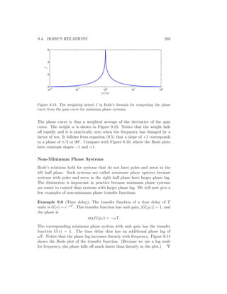
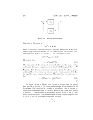
311. 9.6. FURTHER READING 299
Notice that if systems H1 and H2 are linear it follows from the Nyquist
stability theorem that the closed loop is stable, because if γ1γ2 < 1 the
Nyquist curve is always inside the unit circle. The small gain theorem is
thus an extension of the Nyquist stability theorem.
It also follows from the Nyquist stability theorem that a closed loop
system is stable if the phase of the loop transfer function is between −π and
π. This result can also be extended to nonlinear systems as well. It is called
the passivity theorem and is closely related to the small gain theorem.
Additional applications of the small gain theorem and its application to
robust stability are given in Chapter 12.
9.6 Further Reading
Nyquist’s original paper giving his now famous stability criterion was pub-
lished in the Bell Systems Technical Journal in 1932 [Nyq32].
9.7 Exercises
1. Use the Nyquist theorem to analyze the stability of the speed con-
trol system in Example 9.1, but using the original PI controller from
Example 6.9.
2. Discrete time Nyquist
3. Example systems:

312. 300 CHAPTER 9. LOOP ANALYSIS

313. Chapter 10
PID Control
Based on a survey of over eleven thousand controllers in the refining, chemi-
cals and pulp and paper industries, 97% of regulatory controllers utilize PID
feedback.
Desborough Honeywell, 2000, see [DM02].
PID control is by far the most common way of using feedback in natural
and man-made systems. PID controllers are commonly used in industry
and a large factory may have thousands of them, in instruments and lab-
oratory equipment. In engineering applications the controllers appear in
many different forms: as a stand alone controller, as part of hierarchical,
distributed control systems, or built into embedded components. Most con-
trollers do not use derivative action. In this chapter we discuss the basic
ideas of PID control and the methods for choosing the parameters of the
controllers. Many aspects of control can be understood based on linear
analysis. However, there is one nonlinear effect, that has to be considered in
most control systems namely that actuators saturate. In combinations with
controllers having integral actions saturations give rise to an effect called
integral windup. This phenomenon that occurs in practically all control
systems will be discussed in depth for PID controllers. Methods to avoid
windup will also be presented. Finally we will also discuss implementation
of PID controllers, similar methods can be used to implement many other
controllers.
301

314. 302 CHAPTER 10. PID CONTROL
0000000000
00000
1111111111
11111
000111000000111111
Present
FuturePast
t t + Td
Error
Time
Figure 10.1: A PID controller takes control action based on past, present and
prediction of future control errors.
10.1 The Controller
The ideal version of the PID controller is given by the formula
u(t) = kpe(t) + ki
t
0
e(τ) dτ + kd
de
dt
, (10.1)
where u is the control signal and e is the control error (e = r − y). The
reference value, r, is also called the setpoint. The control signal is thus a
sum of three terms: a proportional term that is proportional to the error, an
integral term that is proportional to the integral of the error, and a derivative
term that is proportional to the derivative of the error. The controller
parameters are proportional gain kp, integral gain ki and derivative gain kd.
The controller can also be parameterized as
u(t) = kp e(t) +
1
Ti
t
0
e(τ)dτ + Td
de(t)
dt
, (10.2)
where Ti is the integral time constant and Td the derivative time constant.
The proportional part acts on the present value of the error, the integral
represents an average of past errors and the derivative can be interpreted as
a prediction of future errors based on linear extrapolation, as illustrated in
Figure 10.1. Note that the control signal u is formed entirely from the error
e, there is no feedforward term (which would correspond to krr in the state
feedback case). In Section 10.5 we will introduce a modification which also
uses feedforward.
We begin our analysis by considering pure proportional feedback. Fig-
ure 10.2a shows the responses of the output to a unit step in the command

315. 10.1. THE CONTROLLER 303
0 10 20
0
0.5
1
1.5
0 10 20
−2
0
2
4
t
yu
0 10 20
0
0.5
1
1.5
0 10 20
0
1
2
t
y
u
0 10 20
0
0.5
1
1.5
0 10 20
0
2
4
t
y
u
(a) (b) (c)
Figure 10.2: Responses to step changes in the command signal for a proportional
controller (left), PI controller (center) and PID controller (right). The process
has the transfer function P(s) = 1/(s + 1)3
, the proportional controller (left) had
parameters kp = 1 (dashed), 2 and 5 (dash-dotted), the PI controller has parameters
kp = 1, ki = 0 (dashed), 0.2, 0.5 and 1 (dash-dotted), and the PID controller has
parameters are kp = 2.5, ki = 1.5 and kd = 0 (dashed), 1, 2, 3 and 4 (dash-dotted).
signal for a system with pure proportional control at different gain settings.
In the absence of a feedforward term, the output never reaches the reference
and hence we are left with non-zero steady state error. Letting the pro-
cess and the controller have transfer functions P(s) and C(s), the transfer
function from reference to output is
Gyr =
PC
1 + PC
. (10.3)
The zero frequency gain with proportional control C(s) = kp is
Gyr(0) =
P(0)kp
1 + P(0)kp
and thus the steady state error for a unit step is 1−Gyr(0) = 1/(1+kpP(0)).
For the system in Figure 10.2a with gains kp = 1, 2 and 5, the steady state
error is 0.5, 0.33 and 0.17. The error decreases with increasing gain, but the
system also becomes more oscillatory. Notice in the figure that the initial
value of the control signal equals the controller gain.

316. 304 CHAPTER 10. PID CONTROL
ΣK
e u
1
1 + sTi
u y
1
− 1
1+sT
Σ
(a) (b)
Figure 10.3: Implementation of integral action (left) and derivative action (right)
by combining simple blocks.
To avoid having a steady state error, the proportional controller can be
changed to
u(t) = kpe(t) + ud, (10.4)
where ud is a feedforward term that is adjusted to give the desired steady
state value. If we choose ud = r/P(0) = krr, then the output will be exactly
equal to the reference value, as it was in the state space case. However,
this requires exact knowledge of the process dynamics, which is usually not
available. In early controllers the term ud, which was also called the reset,
was adjusted manually to obtain the desired steady state.
As we saw in Sections 1.5 and 6.4, integral action guarantees that the
process output agrees with the reference in steady state and provides an
alternative to including a feedforward term. To see the effect of integral
action in the frequency domain, we consider a proportional-integral (PI)
controller, which has a transfer function
C(s) = kpe +
ki
s
.
We see that the controller has infinite zero frequency gain (C(0) = ∞) and
it then follows from equation (10.3) that Gyr(0) = 1, which implies that
there is no steady-state error.
Integral action can also be viewed as a method for generating the feed-
forward term ud in the proportional controller (10.4) automatically. An
alternative way to represent this action is shown in Figure 10.3a, where the
low pass part of the control action of a proportional controller is filtered and
feed back with positive gain. This implementation, called automatic reset,
was one of the early inventions of integral control. Integral action is often
realized in this way in biological systems.

317. 10.1. THE CONTROLLER 305
The transfer function of the system in Figure 10.3 is obtained by loop
tracing: assuming exponential signals, we have
u = kpe +
1
1 + sT
u,
and solving for u gives
u = kp
1 + sT
sT
e = kp +
kp
sT
,
which is the transfer function for a PI controller.
The properties of integral action are illustrated in Figure 10.2b. The
proportional gain is constant, kp = 1, and the integral gains are ki = 0, 0.2,
0.5 and 1. The case ki = 0 corresponds to pure proportional control, with a
steady state error of 50%. The steady state error is removed when integral
gain action is used. The response creeps slowly towards the reference for
small values of ki, but faster for larger integral gains, but the system also
becomes more oscillatory.
We now return to the general PID controller and consider the use of
the derivative term, kd. Recall that the original motivation for derivative
feedback was to provide predictive action. The input-output relation of a
controller with proportional and derivative action is
u = kpe + kd
de
dt
= k e + Td
de
dt
,
where Td = kd/kp is the derivative time constant. The action of a controller
with proportional and derivative action can be interpreted as if the control
is made proportional to the predicted process output, where the prediction
is made by extrapolating the error Td time units into the future using the
tangent to the error curve (see Figure 10.1).
Derivative action can also be implemented by taking the difference be-
tween the signal and its low-pass filtered version as shown in Figure 10.3a.
The transfer function for the system is
C(s) = 1 −
1
1 + sT
=
sT
1 + sT
U(s).
The system thus has the transfer function G(s) = sT/(1 + sT), which ap-
proximates a derivative for low frequencies. Notice that this implementation
gives filtering automatically.
Figure 10.2c illustrates the behavior of a system with a PID controller:
the system is oscillatory when no derivative action is used and it becomes

318. 306 CHAPTER 10. PID CONTROL
more damped as derivative gain is increased. A comparison of the systems
with P, PI and PID control in Figure 10.2 shows that the steady-state error
is removed by introducing integral action and that the response speed can
be improved by introducing derivative action.
10.2 Tuning
Users of control systems are frequently faced with the task of adjusting
the controller parameters to obtain a desired behavior. There are many
different ways to do this. One way to do this is to go through the steps of
modeling and control design. Since the PID controller has so few parameters
a number of special empirical methods have also been developed. A simple
idea is to connect a controller, increase the gain until the the system starts
to oscillate, and then reduce the gains by an appropriate factor. Another
is to measure some features of the open loop response and to determine
controller parameters based on these features. We will present the Ziegler-
Nichols methods which are the most celebrated tuning rules.
Ziegler-Nichols’ Tuning
Ziegler and Nichols develped two techniques for controller tuning in the
1940s. The idea was to tune the controller based on the following idea: Make
a simple experiment, extract some features of process dynamics from the
experimental data, and determine controller parameters from the features.
One method is based on direct adjustment of the controller parameters.
A controller is connected to the process, integral and derivative gain are
set to zero and the proportional gain is increased until the system starts
to oscillate. The critical value of the proportional gain kc is observed to-
gether with the period of oscillation Tc. The controller parameters are then
given by Table 10.1. The values in the table were obtained based on many
simulations and experiments on processes that are normally encountered in
process industry. There are many variations of the method which are widely
used in industry.
Another method proposed by Ziegler and Nichols is based on determi-
nation of the open loop step response of the process, as shown Figure 10.4a.
The step response is measured by applying a step input to the process and
recording the response. The response is scaled to correspond to a unit step
input and characterized by parameters a and Tdel, which are the intercepts
of the steepest tangent of the step response with the coordinate axes. The
parameter Tdel is an approximation of the time delay of the system and

319. 10.2. TUNING 307
Table 10.1: Controller parameters for the Ziegler-Nichols frequency response
method which gives controller parameters in terms of critical gain kc and criti-
cal period Tc. Parameter Tp is an estimate of the period of damped oscillations of
the closed loop system.
Controller kp/kc Ti/Tc Td/Tc Tp/Tc
P 0.5 1.0
PI 0.4 0.8 1.4
PID 0.6 0.5 0.125 0.85
a/Tdel is the steepest slope of the step response. Notice that it is not nec-
essary to wait until steady state to find the parameters, it suffices to wait
until the response has had an inflection point. The controller parameters are
given in Table 10.2. The parameters were obtained by extensive simulation
of a range of representative processes.
Improved Ziegler-Nichols Rules
There are two drawbacks with the Ziegler-Nichols rules: too little process
information is used and the closed loop systems that are obtained lack ro-
bustness. Substantially better tuning is obtained by fitting the model
P(s) =
K
1 + sT
e−sTdel
(10.5)
to the step response. A simple way to do this is illustrated in Figure 10.4b.
The zero frequency gain of the process K is determined from the steady
state value of the step response. The time delay Tdel is determined from the
tTdel
y
−a
(a)
tTdel
y
K
0.63K
T63
(b)
Figure 10.4: Characterization of the unit step response by two (left) and three
parameters (right). The point where the tangent is steepest is marked with a small
circle.

320. 308 CHAPTER 10. PID CONTROL
Table 10.2: Controller parameters for the Ziegler-Nichols step response method.
Parameter Tp is an estimate of the period of damped oscillations of the closed loop
system.
Controller akp Ti/Tdel Td/Tdel Tp/Tdel
P 1 4
PI 0.9 3 5.7
PID 1.2 2 Tdel/2 3.4
intercept of the steepest tangent to the step response and the time T63 is
the time where the output has reached 63% of its steady state value. The
parameter T is then given by T = T63 − Tdel. Notice that the experiment
takes longer time than the experiment in Figure 10.4a because it is neces-
sary to wait until the steady state has been reached. The following tuning
formulas have been obtained by tuning controllers to a large set of processes
typically encountered in process control
kpK = min 0.4 T/L, 0.25
Ti = max (T, 0.5Tdel).
(10.6)
Notice that the improved formulas typically give lower controller gain than
the Ziegler-Nichols method, and that integral gain is higher, particularly for
systems with dynamics that are delay dominated, i.e. Tdel > 2T.
Relay Feedback
The experiment used in the Ziegler-Nichols frequency response method,
where the gain of a proportional controller is increased until the system
reaches instability, gives the frequency ω180 where the process has a phase
lag of 180◦ and the process gain K180at that frequency. Another way to
obtain this information is to connect the process in a feedback loop with
a relay as shown in Figure 10.5a. For many systems there will then be an
oscillation, as shown in Figure 10.5b, where the relay output u is a square
wave and the process output y is close to a sinusoid. Notice that the process
input and output have opposite phase and that an oscillation with constant
period is established quickly.
To provide some analysis, we assume that the relay output is expanded in
a Fourier series and that the process attenuates higher harmonics effectively.
It is then sufficient to consider only the first harmonic component of the

321. 10.3. MODELING AND CONTROL DESIGN 309
G(s)
yueysp
−1 0 10 20 30
−1
−0.5
0
0.5
1
y
t
(a) (b)
Figure 10.5: Block diagram of a process with relay feedback (left) and typical signals
(right). The process output y is solid and the relay output u is dashed. Notice that
the signals u and y are out of phase.
input. The input and the output then have opposite phase, which means
that the frequency of the oscillation ω180 is such that the process has a phase
lag of 180◦. If d is the relay amplitude, the first harmonic of the square wave
input has amplitude 4d/π. Let a be the amplitude of the process output.
The process gain at ω180 is then given by
K180 = |P(iω180| =
πa
4d
. (10.7)
The relay experiment is easily automated. Since the amplitude of the oscil-
lation is proportional to the relay output, it is easy to control it by adjusting
the relay output. The amplitude and the period can be determined after
about 20 s, in spite of the fact that the system is started so far from the
equilibrium that it takes about 8 s to reach the correct level. The settling
time for the step response of the system is 40 s.
Automatic tuning based on relay feedback is used in many commercial
PID controllers. Tuning is accomplished simply by pushing a button which
activates relay feedback. The relay amplitude is automatically adjusted to
keep the oscillations sufficiently small, the relay feedback is switched to a
PID controller as soon as the tuning is accomplished.
10.3 Modeling and Control Design
Parameters of PID controllers can also be determined by modeling process
dynamics and applying some method for control design. Since the complex-
ity of the controller is directly related to the complexity of the model it is
necessary to have models of low order.
To illustrate the ideas we will consider the case where a process dynamics

322. 310 CHAPTER 10. PID CONTROL
is approximated by a first order transfer function
P(s) =
b
s + a
.
The approximation is reasonable for systems where storage of mass, momen-
tum and energy can be captured by one state variable. Typical examples
are the velocity of a car on the road, control of the velocity of a rotating
system, electric systems where energy is essentially stored in one compo-
nent, incompressible fluid flow in a pipe, level control of a tank, pressure
control in a gas tank and temperature in a body with uniform temperature
distribution.
A PI controller has the transfer function
C(s) = kp +
ki
s
,
and the transfer function of the closed loop system from reference to output
is
Gyr =
PC
1 + PC
=
b(kps + ki)
s2 + (a + bkp)s + bki
.
The closed loop system has the characteristic polynomial
s2
+ (a + bkp)s + bki.
Assuming that the desired characteristic polynomial is
s2
+ 2ζω0s + ω2
0, (10.8)
we find that the controller parameters are given by
kp =
2ζω0 − a
b
=
2ζω0T − 1
K
ki =
ω2
0
b
=
ω2
0T
K
.
(10.9)
The parameter ω0 determines the response speed and ζ determines the
damping. Notice that controller gain becomes negative if ζω0 < 0.5, which
gives a closed loop system with bad properties, as will be discussed in Sec-
tion 12.5.
The same approach can be used to find the parameters of a PID controller
for a process with dynamics of second order (Exercise 1).

323. 10.3. MODELING AND CONTROL DESIGN 311
Example 10.1 (Cruise control design). Consider the problem of maintain-
ing the speed of a car as it goes up a hill. In Example 5.14we found that
there was very little difference between the linear and nonlinear models when
investigating PI control provided that the throttle does not reach the satu-
ration limits. We will now use a linear model to design a controller and to
investigate the effects of design parameters. A simple linear model of a car
was given in Example 5.10:
d(v − ve)
dt
= a(v − ve) + b(u − ue) − gθ, (10.10)
where v is the velocity of the car, u is the input from the engine and θ
is the slope of the hill. The parameters were a = −0.101, b = 1.3203,
g = 9.8, ve = 20, and ue = 0.1616. This model will be used to find suitable
parameters of a vehicle speed controller. To investigate the behavior of the
closed loop system we start with the linearized process model (10.10) and
we assume that the cruise controller is PI controller is described by
u = kp(ve − v) + ki
t
0
(ve − v(τ))dτ. (10.11)
To compute the error dynamics, introduce the error e = ve − v, differentiate
equations (10.10) and (10.11), and eliminate u. The error is then given by
the differential equation
d2e
dt2
+ (−a + bkp)
de
dt
+ bkie = 9.8
dθ
dt
. (10.12)
We notice that the steady state error is zero if θ and e are constant, which
is no surprise since the controller has integral action.
To understand the effects of the controller parameters K and ki we can
compare equation (10.12) with the standard second order system
¨q + 2ζω0 ˙q + ω2
0q = ku.
This gives
kp =
a + 2ζω0
b
ki =
ω2
0
b
where ζ denotes relative damping and ω0 is the undamped natural frequency.
The parameter ω0 gives response speed and ζ determines the shape of the
response. Since it is desirable that a cruise control system should respond to
changes smoothly without oscillations we choose ζ = 1, which corresponds
to critical damping.

324. 312 CHAPTER 10. PID CONTROL
0 10 20 30 40
−1.5
−1
−0.5
0
0 10 20 30 40
0
0.2
0.4
0.6
0.8
throttle
t [s]
v[m/s]
0 10 20 30 40
−1
−0.5
0
0.5
0 10 20 30 40
0
0.2
0.4
0.6
0.8
throttle
t [s]
v[m/s]
Figure 10.6: Illustrates the effect of parameters ω0 (left) and ζ0 (right) on the
response of a car with cruise control.
The consequences of different choices of ω0 and ζ0 are illustrated in
Figure 10.6. The figure shows the velocity and throttle for a car that first
moves on a horizontal road and encounters a hill with slope 4◦ at time 6.
Between time 5 and 6 the slope increases linearly. The choice of ω0 is a
compromise between response speed and control actions. The compromise
is illustrated in Figure 10.6, which shows the velocity error and the control
signal for a simulation where the slope of the road suddenly changes by 4◦.
The largest velocity error decreases with increasing ω0, but the control signal
also changes more rapidly. In the simple model (10.10) it was assumed that
the force responds instantaneously to throttle commands. For rapid changes
there may be additional dynamics that has to be accounted for. There are
also physical limitations to the rate of change of the force, which also restrict
the admissible value of ω0. A reasonable choice of ω0 is in the range of 0.2
to 1.0. Notice in Figure 10.6 that even with ω0 = 0.1 the largest velocity
error is only 1 m/s.
Another interpretation of the effect of the integral action can be given
by returning to the basic force balance model of the car
m
dv
dt
= F − Fd,
where m is the mass of the car, F is the applied force (from the engine)
and Fd is the disturbance force (aerodynamic drag and force of gravity).
Since zero steady state error implies that v is constant, we see that the PI
controller generates an output force F that in steady state is equal to the

325. 10.4. INTEGRATOR WINDUP 313
drag force Fd. Since the error is zero in steady state the controller output
equals the output of the integrator of the PI controller. The output of the
integrator in the PI controller can thus be interpreted as an estimator of the
drag force. ∇
10.4 Integrator Windup
Many aspects of a control system can be understood from linear models.
There are, however, some nonlinear phenomena that must be taken into ac-
count. These are typically limitations in the actuators: a motor has limited
speed, a valve cannot be more than fully opened or fully closed, etc. For
a system which operates over a wide range of conditions, it may happen
that the control variable reaches the actuator limits. When this happens
the feedback loop is broken and the system runs in open loop because the
actuator will remain at its limit independently of the process output as long
as the actuator remains saturated. The integral term will also build up since
the error typicallys zero. The integral term and the controller output may
then become very large. The control signal will then remain saturated even
when the error changes and it may take a long time before the integrator and
the controller output comes inside the saturation range. The consequence is
that there are large transients. This situation is colloquially referred to as
integrator windup which is illustrated by the following example.
Example 10.2 (Cruise control). The windup effect is illustrated in Fig-
ure 10.7, which shows what happens when a car encounters a hill that is
so steep (6◦) that the throttle saturates when the cruise controller attempts
to maintain speed. When encountering the slope at time t = 5 the velocity
decreases and the throttle increases to generate more torque. The torque
required is however so large that the throttle saturates. The error decreases
slowly because the torque generated by the engine is just a little larger than
the torque required to compensate for the gravity. The error is large and
the integral continues to build up until the error reaches zero at time 30, but
but the controller output is still much larger than the saturation limit and
the actuator remains saturated. The integral term starts to decrease and at
time 45 and the velocity settles to quickly to the desired value. Notice that
it takes considerable time before the controller output comes in the range
where it does not saturate resulting in a large overshoot. ∇

326. 314 CHAPTER 10. PID CONTROL
0 20 40 60
18
19
20
21
0 20 40 60
0
0.5
1
1.5
2
2.5
Velocity[m/s]Throttle
Time [s]
(a)
0 20 40 60
18
19
20
21
0 20 40 60
0
0.5
1
1.5
2
2.5
Velocity[m/s]Throttle
Time [s]
(b)
Figure 10.7: Simulation of windup (left) and anti-windup (right). The figure shows
the speed v and the throttle u for a car that encounters a slope that is so steep that
the throttle saturates. The controller output is dashed. The controller parameters
are kp = 0.5 and ki = 0.1.
Avoiding Windup
There are many ways to avoid windup. One method is illustrated in Fig-
ure 10.8: the system has an extra feedback path that is generated by mea-
suring the actual actuator output, or the output of a mathematical model
of the saturating actuator, and forming an error signal (es) as the difference
between the output of the controller (v) and the actuator output (u). The
signal es is fed to the input of the integrator through gain kt. The signal
es is zero when there is no saturation and the extra feedback loop has no
effect on the system. When the actuator saturates, the signal es is feedback
to the integrator in such a way that es goes towards zero. This implies that
controller output is kept close to the saturation limit. The controller output
will then change as soon as the error changes sign and integral windup is
avoided.
The rate at which the controller output is reset is governed by the feed-
back gain, kt, a large value of kt give a short reset time. The parameter kt
can, however, not be too large because measurement error can then cause
an undesirable reset. A reasonable compromise is to choose kt ≈ 1/Ti for PI
control and as kt ≈ 1/
√
TiTd for PID control. We illustrate how integral
windup can be avoided by investigating the cruise control system.
Example 10.3 (Cruise control). Figure 10.7b shows what happens when

327. 10.5. IMPLEMENTATION 315
− +
Σ
Σ
Σ
Actuator
model Actuator
−y
e = ysp − y
ki
kd
1
s
kt
es
k
v u
Figure 10.8: PID controller with anti-windup.
a controller with anti-windup is applied to the system simulated in Fig-
ure 10.7a. Because of the feedback from the actuator model the output of
the integrator is quickly reset to a value such that the controller output is
at the saturation limit. The behavior is drastically different from that in
Figure 10.7a and the large overshoot is avoided. The tracking gain kt = 2
in the simulation. ∇
10.5 Implementation
There are many practical issues that have to be considered when implement-
ing PID controllers. They have been developed over time based on practical
experiences. In this section we consider some of the most common. Similar
considerations also apply to other types of controllers.
Filtering the Derivative
A drawback with derivative action is that an ideal derivative has very high
gain for high frequency signals. This means that high frequency measure-
ment noise will generate large variations of the control signal. The effect of
measurement noise be reduced by replacing the term kds by
Da = −
kds
1 + sTf
. (10.13)
This can be interpreted as an ideal derivative that is filtered using a first-
order system with the time constant Tf . For small s the transfer function is

328. 316 CHAPTER 10. PID CONTROL
approximately kds and for large s it is equal to kd/Tf . The approximation
acts as a derivative for low-frequency signals and as a constant gain for
the high frequency signals. The filtering time is chosen as Tf = (kd/k)/N,
with N in the range of 2 to 20. Filtering is obtained automatically if the
derivtive is implemented by taking difference between the signal and a its
filtered version as shown in Figure 10.2.
The transfer function of a PID controller with a filtered derivative is
C(s) = kp 1 +
1
sTi
+
sTd
1 + sTd/N
. (10.14)
The high-frequency gain of the controller is K(1 + N). Instead of filtering
just the derivative it is also possible to use an ideal controller and filter the
measured signal. The transfer function of such a controller with the filter is
then
C(s) = kp 1 +
1
sTi
+ sTd
1
(1 + sTf )2
. (10.15)
where a second order filter is used.
Setpoint Weighting
The control system in equation (10.1) is called a system with error feedback
because the controller acts on the error, which is the difference between the
reference and the output. In the simulation of PID controllers in Figure 10.1
there is a large initial peak of the control signal, which is caused by the
derivative of the reference signal. The peak can be avoided by modifying
the controller equation (10.1) to
u = kp βr − y + ki
∞
0
r(τ) − y(τ) dτ + kd γ
dr
dt
−
dy
dt
(10.16)
In this controller, proportional and derivative actions act on fractions β and
γ of the reference. Integral action has to act on the error to make sure that
the error goes to zero in steady state. The closed loop systems obtained for
different values of β and γ respond to load disturbances and measurement
noise in the same way. The response to reference signals is different because
it depends on the values of β and γ, which are called reference weights or
setpoint weights.
Figure 10.9 illustrates the effects of setpoint weighting on the step re-
sponse. The figure shows clearly the effect of changing β. The overshoot for
reference changes is smallest for β = 0, which is the case where the refer-
ence is only introduced in the integral term, and increases with increasing

329. 10.5. IMPLEMENTATION 317
0 2 4 6 8
0
0.5
1
1.5
0 2 4 6 8
−0.5
0
0.5
1
1.5
uy
t
10
−1
10
0
10
1
10
−1
10
0
10
−1
10
0
10
1
10
−1
10
0
ω
|Gyr(jω)||Gur(jω)|
Figure 10.9: Time and frequency responses for system with PI controller and set-
point weighting. The curves on the left show responses in process output y and
control signal and the curves on the right show the gain curves for the transfer
functions Gyr(s) and Gur(s). The process transfer function is P(s) = 1/s, the con-
troller gains are k = 1.5 and ki = 1, and the setpoint weights are β = 0 (dashed)
0.2, 0.5 and 1 (dash dotted).
β. Parameter β it typically in the range of 0 to 1 and γ is normally zero to
avoid large transients in the control signal when the reference is changed.
The controller given by equation (10.16) is a special case of controller
with two degrees which will be discussed in Section 11.1.
Implementation based Operational Amplifiers
PID controllers have been implemented in many different technologies. Fig-
ure 10.10 shows how they can be implemented by feedback around opera-
tional amplifiers.
To show that the circuit in Figure 10.10b is a PID controller we will
use the approximate relation between the input voltage e and the output
voltage u of an operational amplifier in Section 3.3:
u = −
Z1
Z0
e,
where Z0 is the impedance between the negative input of the amplifier and
the input voltage e, and Z1 is the impedance between the zero input of the

330. 318 CHAPTER 10. PID CONTROL
R0 R1 C1
e
u
R0 R1
C0
C1
e
u
(a) (b)
Figure 10.10: Schematic diagram of an electronic PI (left) and PID controllers
(right) based on feedback around an operational amplifier.
amplifier and the output voltage u. The impedances are given by
Z0 =
R0
1 + R0C0p
Z1 = R1 +
1
C1p
,
and we find the following relation between the input voltage e and the output
voltage u:
u = −
Z1
Z0
e = −
R1
R0
(1 + R0C0p)(1 + R1C1p)
R1C1p
e.
This is the input-output relation for a PID controller on the form (10.2)
with parameters
kp =
R1
R0
Ti = R1C1 Td = R0C0.
The corresponding results for a PI controller is obtained by setting C0 = 0.
Computer Implementation
In this section we briefly describe how a PID controller may be implemented
using a computer. The computer typically operates periodically, with sig-
nals from the sensors sampled and converted to digital form by the A/D
converter, the control signal computed and then converted to analog form
for the actuators. The sequence of operation is as follows:
1. Wait for clock interrupt
2. Read input from sensor
3. Compute control signal
4. Send output to the actuator
5. Update controller variables

331. 10.5. IMPLEMENTATION 319
6. Repeat
Notice that an output is sent to the actuators as soon as it is available. The
time delay is minimized by making the calculations in Step 3 as short as
possible and performing all updates after the output is commanded.
As an illustration we consider the PID controller in Figure 10.8, which
has a filtered derivative, setpoint weighting and protection against integral
windup. The controller is a continuous time dynamical system. To imple-
ment it using a computer, the continuous time system has to be approxi-
mated by a discrete time system.
The signal v is the sum of the proportional, integral and derivative terms
v(t) = P(t) + I(t) + D(t) (10.17)
and the controller output is u(t) = sat(v(t)) where sat is the saturation
function that models the actuator. The proportional term is
P = kp(βysp − y).
This term is implemented simply by replacing the continuous variables with
their sampled versions. Hence
P(tk) = kp (βyr(tk) − y(tk)) , (10.18)
where {tk} denotes the sampling instants, i.e., the times when the computer
reads its input. The integral term is
I(t) = ki
t
0
e(s)ds +
1
Tt
sat(v) − v)
and approximating the integral by a sum gives
I(tk+1) = I(tk) + kih e(tk) +
h
Tt
sat(v) − v) . (10.19)
The derivative term D is given by the differential equation
Tf
dD
dt
+ D = −kdy.
Approximating this equation with a backward difference we find
Tf
D(tk) − D(tk−1)
h
+ D(tk) = −kd
y(tk) − y(tk−1)
h
,

332. 320 CHAPTER 10. PID CONTROL
which can be rewritten as
D(tk) =
Tf
Tf + h
D(tk−1) −
kd
Tf + h
(y(tk) − y(tk−1)) . (10.20)
The advantage of using a backward difference is that the parameter Tf /(Tf +
h) is nonnegative and less than one for all h > 0, which guarantees that the
difference equation is stable.
Reorganizing equations (10.17)–(10.20), the PID controller can be de-
scribed by the following pseudo code:
% Precompute controller coefficients
bi=ki*h
ad=Tf/(Tf+h)
bd=kd/(Tf+h)
br=h/Tt
% Control algorithm - main loop
while (running) {
r=adin(ch1) % read setpoint from ch1
y=adin(ch2) % read process variable from ch2
P=kp*(b*r-y) % compute proportional part
D=ad*D-bd*(y-yold) % update derivative part
v=P+I+D % compute temporary output
u=sat(v,ulow,uhigh) % simulate actuator saturation
daout(ch1) % set analog output ch1
I=I+bi*(r-y)+br*(u-v) % update integral
yold=y % update old process output
sleep(h) % wait until next update interval
}
Precomputation of the coefficients bi, ad, bd and br saves computer time
in the main loop. These calculations have to be done only when controller
parameters are changed. The main loop is executed once every sampling
period. The program has three states: yold, I, and D. One state variable
can be eliminated at the cost of a less readable code. Notice that the code
includes computing the derivative of the process output, proportional action
on a portion of the error (b = 1), and modeling of the actuator saturation
in the integral computation to give protection against windup.
10.6 Further Reading
The history of PID control is a very rich one and stretches back to the
beginning of the foundation of control theory. A very readable treatment is

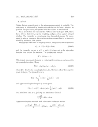
333. 10.7. EXERCISES 321
given by Mindel [Min02]. A comprehensive presentation of PID control is
given in [˚AH95].
10.7 Exercises
1. Consider a second order process with transfer function
P(s) =
b
s2 + a1s + a2
.
Find the gains for a PID controller that gives the closed loop system
a characteristic polynomial of the form
s2
+ 2ζω0s + ω2
0.
2. (Vehicle steering) Design a proportion-integral controller for the vehi-
cle steering system that gives closed loop characteristic equation
s3
+ 2ω0s2
+ 2ω0s + ω3
0.

334. 322 CHAPTER 10. PID CONTROL

335. Chapter 11
Loop Shaping
Quotation
Authors, citation.
In this chapter we continue to explore the use of frequency domain tech-
niques for design of feedback systems. We begin with a more thorough
description of the performance specifications for control systems, and then
introduce the concept of “loop shaping” as a mechanism for designing con-
trollers in the frequency domain. We also introduce some fundamental lim-
itations to performance for systems with right half plane poles and zeros.
11.1 A Basic Feedback Loop
In the previous chapter, we considered the use of PID feedback as a mecha-
nism for designing a feedback controller for a given process. In this chapter
we will expand our approach to include a richer repertoire of tools for shap-
ing the frequency response of the closed loop system.
One of the key ideas in this chapter is that we can design the behavior
of the closed loop system by studying the open loop transfer function. This
same approach was used in studying stability using the Nyquist criterion:
we plotted the Nyquist plot for the open loop transfer function to determine
the stability of the closed loop system. From a design perspective, the use
of loop analysis tools is very powerful: since the loop transfer function is
L = PC, if we can specify the desired performance in terms of properties
of L, we can directly see the impact of changes in the controller C. This is
much easier, for example, than trying to reason directly about the response
323

336. 324 CHAPTER 11. LOOP SHAPING
F C P
−1
Σ Σ Σ
r e u ν
d
η
n
y
Controller Process
Figure 11.1: Block diagram of a basic feedback loop.
of the closed loop system, whose transfer function is given by
Gyr =
PC
1 + PC
(assuming F = 1).
We will start by investigating some key properties of the feedback loop.
A block diagram of a basic feedback loop is shown in Figure 11.1. The system
loop is composed of two components, the process and the controller, and the
controller has two blocks: the feedback block C and the feedforward block
F. There are two disturbances acting on the process, the load disturbance, d,
and the measurement noise, n. The load disturbance represents disturbances
that drive the process away from its desired behavior, while the measurement
noise represents the uncertainty in sensing the output of the system. In the
figure, the load disturbance is assumed to act on the process input. This is
a simplification, since disturbances often enter the process in many different
ways, but allows us to streamline the presentation without significant loss
of generality.
The process output η is the real physical variable that we want to con-
trol. Control is based on the measured signal y, where the measurements are
corrupted by measurement noise n. The process is influenced by the con-
troller via the control variable u. The process is thus a system with three
inputs—the control variable u, the load disturbance d and the measurement
noise n—and one output—the measured signal. The controller is a system
with two inputs and one output. The inputs are the measured signal y and
the reference signal r and the output is the control signal u. Note that the
control signal u is an input to the process and the output of the controller,
and that the measured signal is the output of the process and an input to
the controller.

337. 11.1. A BASIC FEEDBACK LOOP 325
The feedback loop in Figure 11.1 is influenced by three external signals,
the reference r, the load disturbance d and the measurement noise n. There
are at least three signals, η, y and u that are of great interest for control,
giving nine relations between the input and the output signals. Since the
system is linear, these relations can be expressed in terms of the transfer
functions. The following relations are obtained from the block diagram in
Figure 11.1:


w
y
u


=


P
1+PC − PC
1+PC
PCF
1+PC
P
1+PC
1
1+PC
PCF
1+PC
− PC
1+PC − C
1+PC
CF
1+PC




d
n
r


. (11.1)
To simplify notations we have dropped the arguments of all transfer func-
tions.
There are several interesting conclusions we can draw from these equa-
tions. First we can observe that several transfer functions are the same and
that all relations are given by the following set of six transfer functions,
which we call the Gang of Six:
PCF
1 + PC
PC
1 + PC
P
1 + PC
CF
1 + PC
C
1 + PC
1
1 + PC
.
(11.2)
The transfer functions in the first column give the response of the process
output and control signal to the setpoint. The second column gives the
same signals in the case of pure error feedback when F = 1. The transfer
function P/(1 + PC), in the third column, tells how the process variable
reacts to load disturbances and the transfer function C/(1 + PC), in the
second column, gives the response of the control signal to measurement
noise. Notice that only four transfer functions are required to describe how
the system reacts to load disturbances and the measurement noise, and that
two additional transfer functions are required to describe how the system
responds to setpoint changes.
The linear behavior of the system is determined by six transfer functions
in equation (11.2) and specifications can be expressed in terms of these trans-
fer functions. The special case when F = 1 is called a system with (pure)
error feedback. In this case all control actions are based on feedback from
the error only and the system is completely characterized by four transfer
functions, namely the four rightmost transfer functions in equation (11.2),

338. 326 CHAPTER 11. LOOP SHAPING
which have specific names:
S =
1
1 + PC
sensitivity function
T =
PC
1 + PC
complementary sensitivity function
PS =
P
1 + PC
load sensitivity function
CS =
C
1 + PC
noise sensitivity function
(11.3)
These transfer functions and their equivalent systems are called the Gang of
Four. The load disturbance sensitivity function is sometimes called the input
sensitivity function and the noise sensitivity function is sometimes called the
output sensitivity function. These transfer functions have many interesting
properties that will be discussed in detail in the rest of the chapter and good
insight into these properties is essential for understanding feedback systems.
The procedure for designing a controller for the system in Figure 11.1
can be divided into two independent steps:
1. Design the feedback controller C that reduces the effects of load dis-
turbances and the sensitivity to process variations without introducing
too much measurement noise into the system.
2. Design the feedforward F to give the desired response to the reference
signal (or setpoint).
The properties of the system can be expressed in terms of properties of the
transfer functions (11.3), as illustrated in the following example.
Example 11.1. Consider the process
P(s) =
1
(s + 1)4
with a PI feedback controller
C(s) = 0.775 +
1
2.05s
and a feedforward controller
F(s) =
1
(0.5s + 1)4
.

339. 11.1. A BASIC FEEDBACK LOOP 327
0 10 20 30
0
0.5
1
1.5
0 10 20 30
0
0.5
1
1.5
0 10 20 30
0
0.5
1
1.5
0 10 20 30
0
0.5
1
1.5
0 10 20 30
0
0.5
1
1.5
0 10 20 30
0
0.5
1
1.5
PCF/(1 + PC) PC/(1 + PC)
C/(1 + PC)
P/(1 + PC)
CF/(1 + PC) 1/(1 + PC)
η/r
−u/d
y/d
u/r
−u/n
y/n
ttt
Figure 11.2: Step responses of the Gang of Six for PI control k = 0.775, Ti = 2.05
of the process P(s) = (s + 1)−4
. The feedforward is designed to give the transfer
function (0.5s + 1)−4
from reference r to output y.
Figures 11.2 and 11.3 show the step and frequency responses for the Gang
of Six and give useful insight into the properties of the closed loop system.
The time responses in Figure 11.2 show that the feedforward gives a
substantial improvement of the response speed as seen by the differences
between the first and second columns. The settling time is substantially
shorter with feedforward, 4 s versus 25 s, and there is no overshoot. This is
also reflected in the frequency responses in Figure 11.3, which show that the
transfer function with feedforward has higher bandwidth and that it has no
resonance peak.
The transfer functions CF/(1 + PC) and −C/(1 + PC) represent the
signal transmission from reference to control and from measurement noise
to control. The time responses in Figure 11.2 show that the reduction in
response time by feedforward requires a substantial control effort. The initial
value of the control signal is out of scale in Figure 11.2 but the frequency
response in Figure 11.3 shows that the high frequency gain of PCF/(1+PC)
is 16, which can be compared with the value 0.78 for the transfer function
C/(1 + PC). The fast response thus requires significantly larger control
signals.
There are many other interesting conclusions that can be drawn from
Figures 11.2 and 11.3. Consider for example the response of the output
to load disturbances expressed by the transfer function P/(1 + PC). The

340. 328 CHAPTER 11. LOOP SHAPING
10
−1
10
0
10
1
10
−1
10
0
10
−1
10
0
10
1
10
−1
10
0
10
−1
10
0
10
1
10
−1
10
0
10
−1
10
0
10
1
10
0
10
1
10
−1
10
0
10
1
10
0
10
1
10
−1
10
0
10
1
10
0
10
1
PCF/(1 + PC) PC/(1 + PC)
C/(1 + PC)
P/(1 + PC)
CF/(1 + PC) 1/(1 + PC)
w/r
−u/d
y/d
u/r
−u/n
y/n
ωωω
Figure 11.3: Gain curves of frequency responses of the Gang of Six for PI control
k = 0.775, Ti = 2.05 of the process P(s) = (s + 1)−4
where the feedforward has
been designed to give the transfer function (0.5s + 1)−4
from reference to output.
frequency response has a pronounced peak 1.22 at ωmax = 0.5 and the corre-
sponding time function has its maximum 0.59 at tmax = 5.2. Notice that the
peaks are of the same magnitude and that the product of ωmaxtmax = 2.6.
Similar relations hold for the other responses. ∇
11.2 Performance Specifications
A key element of the control design process is how we specify the desired
performance of the system. Inevitably the design process requires a tradeoff
between different features of the closed loop system and specifications are
the mechanism by which we describe the desired outcome of those tradeoffs.
Frequency Domain Specifications
One of the main methods of specifying the performance of a system is
through the frequency response of various input/output pairs. Since spec-
ifications were originally focused on setpoint response, it was natural to
consider the transfer function from reference input to process output. For a
system with error feedback, the transfer function from reference to output is
equal to the complementary transfer function, T = PC/(1+PC). A typical
gain curve for this response is shown in Figure 11.4. Good performance

341. 11.2. PERFORMANCE SPECIFICATIONS 329
ωp ωb
Mr
1
1/
√
2
Figure 11.4: Gain curve for transfer function from setpoint to output.
requires that the zero frequency gain is one (so that the output tracks the
reference). Typical specification measures include:
The resonance peak, Mr, is the largest value of the frequency response.
The peak frequency, ωp, is the frequency where the maximum occurs.
The bandwidth, ωb, is the frequency where the gain has decreased to
1/
√
2.
Specifications can also be related to the loop transfer function, L = PC.
Useful features that have been discussed previously are:
The gain crossover frequency, ωgc, is the lowest frequency where the
loop transfer function L has unit magnitude. This is roughly equal to
the frequency where the closed loop gain drops to below 1/
√
2.
The gain margin, gm, is the amount that the loop gain can be increased
before reaching the stability limit. A high gain margin insures that
errors in modeling the gain of the system do not lead to instability.
The phase margin, ϕm, is the amount of phase lag required to reach
the stability limit. A phase margin of 30◦ to 60◦ is typically required
for robustness to modeling errors and non-oscillatory response.
These concepts were given in more detail in Section 9.3.
In addition to specifications on the loop transfer function, there are
also a number of useful specifications on the sensitivity function and the
complementary sensitivity function:
The maximum sensitivity, Ms, is the peak value of the magnitude of
sensitivity function and indicates the maximum amplification from the
reference to the error signal.

342. 330 CHAPTER 11. LOOP SHAPING
The maximum sensitivity frequency, ωms, is the frequency where the
sensitivity function has its maximum.
The sensitivity crossover frequency, ωsc, is the frequency where the
sensitivity function becomes greater than 1 for the first time. Dis-
turbances are attenuated below this frequency and can be amplified
above this frequency.
The maximum complementary sensitivity, Mt, is the peak value of the
magnitude of the complementary sensitivity function. It provides the
maximum amplification from the reference signal to the output signal.
The maximum complementary sensitivity frequency, ωmt, is the fre-
quency where the complementary sensitivity function has its maxi-
mum.
As we will see in the rest of the chapter, these various measures can be used
to gain insights into the performance of the closed loop system and are often
used to specify the desired performance for a control design.
Although we have defined different specifications for the loop transfer
function L, the sensitivity function S and the complementary sensitivity
function T, these transfer functions are all related through a set of algebraic
relationships:
S =
1
1 + L
T =
L
1 + L
S + T = 1.
These relationships can limit the ability to independently satisfy specifica-
tions for the quantities listed above and may require tradeoffs, as we shall
see.
Relations between Time and Frequency Domain Features
In Section 5.3 we described some of the typical parameters that described
the step response of a system. These included the rise time, steady state
error, and overshoot. For many applications, it is natural to provide these
time domain specifications and we can relate these to the eigenvalues of the
closed loop system, which are equivalent to the poles of the transfer function
T = PC/(1 + PC).
There are approximate relations between specifications in the time and
frequency domain. Let G(s) be the transfer function from reference to out-
put. In the time domain the response speed can be characterized by the rise
time Tr and the settling time Ts. In the frequency domain the response time

343. 11.2. PERFORMANCE SPECIFICATIONS 331
can be characterized by the closed loop bandwidth ωb, the gain crossover
frequency ωgc, the sensitivity frequency ωms. The product of bandwidth and
rise time is approximately constant Trωb ≈ 2, so decreasing the rise time
corresponds to increasing the closed loop bandwidth.
The overshoot of the step response Mp is related to the resonant peak Mr
of the frequency response in the sense that a larger peak normally implies
a larger overshoot. Unfortunately there is no simple relation because the
overshoot also depends on how quickly the frequency response decays. For
Mr < 1.2 the overshoot Mp in the step response is often close to Mr − 1.
For larger values of Mr the overshoot is typically less than Mr − 1. These
relations do not hold for all systems: there are systems with Mr = 1 that
have a positive overshoot. These systems have transfer functions that decay
rapidly around the bandwidth. To avoid overshoot in systems with error
feedback it is advisable to require that the maximum of the complementary
sensitivity function is small, say Mt = 1.1 − 1.2.
Response to Load Disturbances
The sensitivity function in equation (11.3) shows how feedback influences
disturbances. Disturbances with frequencies that are lower than the sen-
sitivity crossover frequency ωsc are attenuated by feedback and those with
ω > ωsc are amplified by feedback. The largest amplification is the maxi-
mum sensitivity Ms.
Consider the system in Figure 11.1. The transfer function from load
disturbance d to process output w is
Gwd =
P
1 + PC
= PS =
T
C
. (11.4)
Since load disturbances typically have low frequencies, it is natural that the
criterion emphasizes the behavior of the transfer function at low frequen-
cies. Filtering of the measurement signal has only marginal effect on the
attenuation of load disturbances because the filter typically only attenuates
high frequencies. For a system with P(0) = 0 and a controller with integral
action, the controller gain goes to infinity for small frequencies and we have
the following approximation for small s:
Gwd =
T
C
≈
1
C
≈
s
ki
. (11.5)
Figure 11.5 gives the gain curve for a typical case and shows that the ap-
proximation is very good for low frequencies.

344. 332 CHAPTER 11. LOOP SHAPING
10
−3
10
−2
10
−1
10
0
10
1
10
2
10
3
10
−2
10
0
10
−3
10
−2
10
−1
10
0
10
1
10
2
10
3
10
0
10
1
ω
|Gwd(ω)||Gun(ω)|
Figure 11.5: Gains of the transfer functions Gwd and Gun for PID control (k =
2.235, Ti = 3.02, Ti = 0.756 and Tf = Td/5) of the process P = (s + 1)−4
. The
gain of the transfer functions P, C, 1/C are shown with dashed lines and s/ki with
dash-dotted lines.
Measurement noise, which typically has high frequencies, generates rapid
variations in the control variable that are detrimental because they cause
wear in many actuators and they can even saturate the actuator. It is thus
important to keep the variations in the control signal at reasonable levels—
a typical requirement is that the variations are only a fraction of the span
of the control signal. The variations can be influenced by filtering and by
proper design of the high frequency properties of the controller.
The effects of measurement noise are captured by the transfer function
from measurement noise to the control signal,
Gun =
C
1 + PC
= CS =
T
P
. (11.6)
Figure 11.5 shows the gain curve of Gun for a typical system. For low
frequencies the transfer function the sensitivity function equals 1 and equa-
tion (11.6) can be approximated by 1/P. For high frequencies is is approxi-
mated as Gun ≈ C. A simple measure of the effect of measurement noise is
the high frequency gain of the transfer function Gun,
Mun := Gun ∞ = sup
ω
|Gun(jω)|. (11.7)

345. 11.2. PERFORMANCE SPECIFICATIONS 333
1/Ms ωms
ωsc
−1
Figure 11.6: Nyquist curve of loop transfer function showing graphical interpre-
tation of maximum sensitivity. The sensitivity crossover frequency ωsc and the
frequency ωms where the sensitivity has its largest value are indicated in the figure.
All points inside the dashed circle have sensitivities greater than 1.
The sensitivity function can be written as
S =
1
1 + PC
=
1
1 + L
. (11.8)
Since it only depends on the loop transfer function it can also be visualized
graphically using the Nyquist plot of the loop transfer function. This is
illustrated in Figure 11.6. The complex number 1+L(jω) can be represented
as the vector from the point −1 to the point L(jω) on the Nyquist curve.
The sensitivity is thus less than one for all points outside a circle with radius
1 and center at −1. Disturbances of these frequencies are attenuated by the
feedback. If a control system has been designed based on a given model, it
is straightforward to estimate the potential disturbance reduction simply by
recording a typical output and filtering it through the sensitivity function.
Example 11.2. Consider the same system as the previous example
P(s) =
1
(s + 1)4
,
with a PI controller. Figure 11.7 shows the gain curve of the sensitivity
function for k = 0.8 and ki = 0.4. The figure shows that the sensitivity
crossover frequency is 0.32 and that the maximum sensitivity 2.1 occurs at

346. 334 CHAPTER 11. LOOP SHAPING
10
−2
10
−1
10
0
10
1
10
−2
10
−1
10
0
10
1
ω
|S(jω)|
Figure 11.7: Gain curve of the sensitivity function for PI control (k = 0.8, ki = 0.4)
of process with the transfer function P(s) = (s + 1)−4
. The sensitivity crossover
frequency is indicated by + and the maximum sensitivity by o.
ωms = 0.56. Feedback will thus reduce disturbances with frequencies less
than 0.32 rad/s, but it will amplify disturbances with higher frequencies.
The largest amplification is 2.1. ∇
11.3 Feedback Design via Loop Shaping
One advantage the the Nyquist stability theorem is that it is based on the
loop transfer function, which is related to the controller transfer function
through L = PC. It is thus easy to see how the controller influences the
loop transfer function. To make an unstable system stable we simply have
to bend the Nyquist curve away from the critical point.
This simple idea is the basis of several different design methods, collec-
tively called loop shaping. The methods are based on the idea of choosing a
compensator that gives a loop transfer function with a desired shape. One
possibility is to start with the loop transfer function of the process and mod-
ify it by changing the gain and adding poles and zeros to the controller until
the desired shape is obtained.
Design Considerations
We will first discuss suitable forms of a loop transfer function that give
good performance and good stability margins. Good robustness requires
good gain and phase margins. This imposes requirements on the loop trans-
fer function around the crossover frequencies ωpc and ωgc. The gain of L
at low frequencies must be large in order to have good tracking of com-
mand signals and good rejection of low frequency disturbances. This can be

347. 11.3. FEEDBACK DESIGN VIA LOOP SHAPING 335
Figure 11.8: Gain curve of the Bode plot for a typical loop transfer function. The
gain crossover frequency ωgc and the slope ngc of the gain curve at crossover are
important parameters.
achieved by having a large crossover frequency and a steep slope of the gain
curve for the loop transfer function at low frequencies. To avoid injecting
too much measurement noise into the system it is desirable that the loop
transfer function have a low gain at frequencies higher than the crossover
frequencies. The loop transfer function should thus have the shape indicated
in Figure 11.8.
Bode’s relations (see Section 9.4) impose restrictions on the shape of the
loop transfer function. Equation (9.5) implies that the slope of the gain
curve at gain crossover cannot be too steep. If the gain curve is constant,
we have the following relation between slope ngc and phase margin ϕm:
ngc = −2 +
2ϕm
π
. (11.9)
This formula holds approximately when the gain curve does not deviate too
much from a straight line. It follows from equation (11.9) that the phase
margins 30◦, 45◦ and 60◦ corresponds to the slopes -5/3, -3/2 and -4/3.
There are many specific design methods that are based on loop shaping.
We will illustrate the basic approach by the design of a PI controller.
Example 11.3 (Design of a PI controller). Consider a system with the

348. 336 CHAPTER 11. LOOP SHAPING
transfer function
P(s) =
1
(s + 1)4
. (11.10)
A PI controller has the transfer function
C(s) = k +
ki
s
= k
1 + sTi
sTi
.
The controller has high gain at low frequencies and its phase lag is negative
for all parameter choices. To have good performance it is desirable to have
high gain and a high gain crossover frequency. Since a PI controller has
negative phase, the gain crossover frequency must be such that the process
has phase lag smaller than 180−ϕm, where ϕm is the desired phase margin.
For the process (11.10) we have
∠P(jω) = −4 arctan ω
If a phase margin of π/3 or 60◦ is required, we find that the highest gain
crossover frequency that can be obtained with a proportional controller is
ωgc = tan π/6 = 0.577. The gain crossover frequency must be lower with a
PI controller.
A simple way to design a PI controller is to specify the gain crossover
frequency to be ωgc. This gives
L(jω) = P(jω)C(jω) =
kP(jω) 1 + ω2
gcT2
i
ωgcTi
= 1,
which implies
kp =
1 + ω2
gcT2
i
ωgcTiP(jωgc)
.
We have one equation for the unknowns k and Ti. An additional condition
can be obtained by requiring that the PI controller have a phase lag of 45◦
at the gain crossover, hence ωTi = 0.5. Figure 11.9 shows the Bode plot of
the loop transfer function for ωgc = 0.1, 0.2, 0.3, 0.4 and 0.5. The phase
margins corresponding to these crossover frequencies are 94◦, 71◦, 49◦, 29◦
and 11◦. The gain crossover frequency must be less than 0.26 to have the
desired phase margin 60◦. Figure 11.9 shows that the controller increases
the low frequency gain significantly at low frequencies and that the the phase
lag decreases. The figure also illustrates the tradeoff between performance
and robustness. A large value of ωgc gives a higher low frequency gain and

349. 11.3. FEEDBACK DESIGN VIA LOOP SHAPING 337
10
−2
10
−1
10
0
10
−1
10
0
10
1
10
2
10
−2
10
−1
10
0
−200
−150
−100
−50
0
|L(ω)|∠L(ω)
ω
Figure 11.9: Bode plot of the loop transfer function for PI control of a process with
the transfer function P(s) = 1/(s + 1)4
with ωgc = 0.1 (dash-dotted), 0.2, 0.3, 0.4
and 0.5. The dashed line in the figure is the Bode plot of the process.
−1.5 −1 −0.5 0 0.5
−1.5
−1
−0.5
0
0.5
,
0 20 40 60
0
0.5
1
1.5
2
y
0 20 40 60
0
0.5
1
1.5
2
t
u
Figure 11.10: Nyquist plot of the loop transfer function for PI control of a process
with the transfer function P(s) = 1/(s + 1)4
with ωgc = 0.1 (dash-dotted), 0.2,
0.3, 0.4 and 0.5 (left) and corresponding step responses of the closed loop system
(right).

350. 338 CHAPTER 11. LOOP SHAPING
a lower phase margin. Figure 11.10 shows the Nyquist plots of the loop
transfer functions and the step responses of the closed loop system. The
responses to command signals show that the designs with large ωgc are too
oscillatory. A reasonable compromise between robustness and performance
is to choose ωgc in the range 0.2 to 0.3. For ωgc = 0.25, the controller
parameters are k = 0.50 and Ti = 2.0. Notice that the Nyquist plot of the
loop transfer function is bent towards the left for low frequencies. This is
an indication that integral action is too weak. Notice in Figure 11.10 that
the corresponding step responses are also very sluggish. ∇
Lead Compensation
A common problem in design of feedback systems is that the phase lag of
the system at the desired crossover frequency is not high enough to allow
either proportional or integral feedback to be used effectively. Instead, one
may have a situation where you need to add phase lead to the system, so
that the crossover frequency can be increased.
A standard way to accomplish this is to use a lead compensator, which
has the form
C(s) = k
s + a
s + b
a < b. (11.11)
The transfer function corresponding to this controller is shown in Figure 11.11.
A key feature of the lead compensator is that it adds phase lead in the fre-
quency range between the pole/zero pair (and extending approximately 10X
in frequency in each direction). By appropriately choosing the location of
this phase lead, we can provide additional phase margin at the gain crossover
frequency.
Because the phase of a transfer function is related to the slope of the
magnitude, increasing the phase requires increasing the gain of the loop
transfer function over the frequency range in which the lead compensation
is applied. Hence we can also think of the lead compensator as changing the
slope of the transfer function and thus shaping the loop transfer function in
the crossover region (although it can be applied elsewhere as well).
Example 11.4 (Pitch control for a ducted fan). Consider the control of the
pitch (angle) of a vertically oriented ducted fan, as shown in Figure 11.12.
We model the system with a second order transfer function of the form
P =
r
Js2 + ds + mgl
,
with the parameters given in Table 11.1. We take as our performance

351. 11.3. FEEDBACK DESIGN VIA LOOP SHAPING 339
10
−1
10
0
10
1
0
20
40
60
80
freq
|C(s)|∠C(s)
a b
Figure 11.11: Frequency response for a lead compensator, C(s) = k(s + a)/(s + b).
specification that we would like less than 1% error in steady state and less
than 10% tracking error up to 10 rad/sec.
The open loop transfer function is shown in Figure 11.13a. To achieve
our performance specification, we would like to have a gain of at least 10 at
a frequency of 10 rad/sec, requiring the gain crossover frequency to be at a
higher frequency. We see from the loop shape that in order to achieve the
adjustable flaps
net thrust
(x, y)
θ
f2
f1
Figure 11.12: Caltech ducted fan with support stand.

352. 340 CHAPTER 11. LOOP SHAPING
Symbol Description Value
m inertial mass of fan, x axis 4.0 kg
J fan moment of inertia, ϕ3 axis 0.0475 kg m2
r nominal distance of flaps from fan pivot 26.0 cm
d angular damping factor 0.001 kg m/s
g gravitational constant 9.8 m/sec2
Table 11.1: Parameter values for the planar ducted fan model which approximate
the dynamics of the Caltech ducted fan.
desired performance we cannot simply increase the gain, since this would
give a very low phase margin. Instead, we must increase the phase at the
desired crossover frequency.
To accomplish this, we use a lead compensator (11.11) with a = 2 and
b = 50. We then set the gain of the system to provide a large loop gain
up to the desired bandwidth, as shown in Figure 11.13b. We see that this
system has a gain of greater than 10 at all frequencies up to 10 rad/sec and
that it has over 40◦ degrees of phase margin. ∇
The action of a lead compensator is essentially the same as that of the
derivative portion of a PID controller. As described in Section 10.5, we
often use a filter for the derivative action of a PID controller to limit the
high frequency gain. This same effect is present in a lead compensator
through the pole at s = b.
Equation (11.11) is a first order lead compensator and can provide up
to 90◦ of phase lead. Higher levels of phase lead can be provided by using a
second order lead compensator:
C = k
(s + a)2
(s + b)2
a < b.
11.4 Fundamental Limitations
Although loop shaping gives us a great deal of flexibility in designing the
closed loop response of a system, there are certain fundamental limits on
what can be achieved. We consider here some of the primary performance
limitations that can occur; additional limitations having to do with robust-
ness are considered in the next chapter.
One of the key limitations of loop shaping occurs when we have the
possibility of cancellation of right half plane poles and zeros. The canceled

353. 11.4. FUNDAMENTAL LIMITATIONS 341
10
−1
10
0
10
1
10
2
10
−3
10
−2
10
−1
10
0
10
1
Gain
Frequency (rad/sec)
10
−1
10
0
10
1
10
2
−150
−100
−50
0
Phase(deg)
Frequency (rad/sec)
10
−1
10
0
10
1
10
2
10
3
10
−2
10
0
10
2
Gain
Frequency (rad/sec)
10
−1
10
0
10
1
10
2
10
3
−150
−100
−50
0
Phase(deg)
Frequency (rad/sec)
Figure 11.13: Control design using a lead compensator: (a) Bode plot for P and
(b) Bode plot for L = PC using a lead compensator.
poles and zeros do not appear in the loop transfer function but they can
appear in the transfer functions from disturbances to outputs or control
signals. Cancellations can be disastrous if the canceled factors are unstable,
as was shown in Section 7.5. This implies that there is a major difference
between minimum phase and non-minimum phase systems.
To explore the limitations caused by poles and zeros in the right half
plane we factor the process transfer function as
P(s) = Pmp(s)Pnmp(s), (11.12)
where Pmp is the minimum phase part and Pnmp is the non-minimum phase
part. The factorization is normalized so that |Pnmp(jω)| = 1 and the sign is
chosen so that Pnmp has negative phase. Requiring that the phase margin
is ϕm we get
arg L(jωgc) = arg Pnmp(jωgc) + arg Pmp(jωgc) + arg C(jωgc) ≥ −π + ϕm,
(11.13)
where C is the controller transfer function. Let ngc be the slope of the gain
curve at the crossover frequency; since |Pnmp(jω)| = 1 it follows that
ngc =
d log |L(jω)|
d log ω
ω=ωgc
=
d log |Pmp(jω)C(jω)|
d log ω
ω=ωgc
.
The slope ngc is negative and larger than −2 if the system is stable. It
follows from Bode’s relations, equation (9.5), that
arg Pmp(jω) + arg C(jω) ≈ ngc
π
2

354. 342 CHAPTER 11. LOOP SHAPING
Combining this with equation (11.13) gives the following inequality for the
allowable phase lag
ϕℓ = − arg Pnmp(jωgc) ≤ π − ϕm + ngc
π
2
. (11.14)
This condition, which we call the crossover frequency inequality, shows that
the gain crossover frequency must be chosen so that the phase lag of the non-
minimum phase component is not too large. To find numerical values we will
consider some reasonable design choices. A phase margin of 45◦ (ϕm = π/4),
and a slope ngc = −1/2 gives an admissible phase lag of ϕℓ = π/2 = 1.57
rad and a phase margin of 45◦ and ngc = −1 gives and admissible phase lag
ϕℓ = π/4 = 0.78 rad. It is thus reasonable to require that the phase lag of
the non-minimum phase part is in the range of 0.5 to 1.6 radians, or roughly
30◦ to 90◦.
The crossover frequency inequality shows that non-minimum phase com-
ponents impose severe restrictions on possible crossover frequencies. It also
means that there are systems that cannot be controlled with sufficient sta-
bility margins. The conditions are more stringent if the process has an
uncertainty ∆P(jωgc). As we shall see in the next chapter, the admissible
phase lag is then reduced by arg ∆P(jωgc).
A straightforward way to use the crossover frequency inequality is to
plot the phase of the transfer function of the process and the phase of the
corresponding minimum phase system. Such a plot, shown in Figure 11.14,
will immediately show the permissible gain crossover frequencies.
As an illustration we will give some analytical examples.
Example 11.5 (Zero in the right half plane). The non-minimum phase part
of the plant transfer function for a system with a right half plane zero is
Pnmp(s) =
z − s
z + s
. (11.15)
where z > 0. The phase lag of the non-minimum phase part is
ϕℓ = − arg Pnmp(jω) = 2 arctan
ω
z
.
Since the phase of Pnmp decreases with frequency, the inequality (11.14)
gives the following bound on the crossover frequency:
ωgc
z
≤ tan
ϕℓ
2
. (11.16)
With reasonable values of ϕℓ we find that the gain crossover frequency must
be smaller than the right half plane zero. It also follows that systems with
slow zeros are more difficult to control than system with fast zeros. ∇

355. 11.4. FUNDAMENTAL LIMITATIONS 343
10
−1
10
0
10
1
10
−2
10
0
10
2
10
−1
10
0
10
1
−300
−200
−100
0
|G(jω)|
ω
∠G(jω)
ϕl
Figure 11.14: Bode plot of process transfer function (full lines) and corresponding
minimum phase transfer function (dashed). The permissible gain crossover fre-
quencies are those for which the difference in phase between the two curves satisfies
equation (11.14).
Example 11.6 (Time delay). The transfer function of a time delay is
P(s) = e−sT
. (11.17)
This is also the non-minimum phase part Pnmp and the corresponding phase
lag is
ϕℓ = − arg Pnmp(jω) = ωT =⇒ wgc ≤
ϕl
T
.
If the transfer function for the time delay is approximated by
e−sT
≈
1 − sT/2
1 + sT/2
,
we find that a time delay T corresponds to a right half plane zero z = 2/T.
A slow zero thus corresponds to a long time delay. ∇
Example 11.7 (Pole in the right half plane). The non-minimum phase part
of the transfer function for a system with a pole in the right half plane is
Pnmp(s) =
s + p
s − p
, (11.18)
where p > 0. The phase lag of the non-minimum phase part is
ϕℓ = − arg Pnmp(jω) = 2 arctan
p
ω

356. 344 CHAPTER 11. LOOP SHAPING
Table 11.2: Achievable phase margin for for ϕm = π/4 and ngc = −1/2 and different
pole-zero ratios p/z.
p/z 0.45 0.24 0.20 0.17 0.12 0.10 0.05
z/p 2.24 4.11 5.00 5.83 8.68 10 20
ϕm 0 30 38.6 45 60 64.8 84.6
and the crossover frequency inequality becomes
ωgc >
p
tan(ϕℓ/2)
.
With reasonable values of ϕℓ we find that the gain crossover frequency should
be larger than the unstable pole. ∇
Example 11.8 (Pole and a zero in the right half plane). The non-minimum
phase part of the transfer function for a system with both poles and zeros
in the right half plane is
Pnmp(s) =
(z − s)(s + p)
(z + s)(s − p)
. (11.19)
The phase lag of this transfer function is
ϕℓ = − arg Pnmp(jω) = 2 arctan
ω
z
+ 2 arctan
p
ω
= 2 arctan
ωgc/z + p/ωgc
1 − p/z
.
The mininum value of the right hand side is given by
min
ωgc
2 arctan
ωgc/z + p/ωgc
1 − p/z
= 2 arctan
2 p/z
1 − p/z
= 4 arctan
p
z
,
which is achieved at ω =
√
pz. The crossover frequency inequality (11.14)
becomes
ϕℓ = − arg Pnmp(jω) ≤ 4 arctan
p
z
,
or
p
z
≤ tan
ϕℓ
4
.
The design choices ϕm = π/4 and ngc = −1/2 gives p < 0.17z. Table 11.2
shows the admissible pole-zero ratios for different phase margins. The

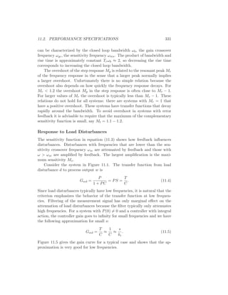
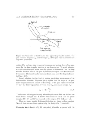
357. 11.5. DESIGN EXAMPLE 345
phase-margin that can be achieved for a given ratio p/z is
ϕm < π + ngc
π
2
− 4 arctan
p
z
. (11.20)
A pair of poles and zeros in the right half plane thus imposes severe con-
straints on the gain crossover frequency. The best gain crossover frequency
is the geometric mean of the unstable pole and zero. A robust controller
does not exist unless the pole/zero ratio is sufficiently small. ∇
Avoiding Difficulties with RHP Poles and Zeros
As the examples above show, right half plane poles and zeros significantly
limit the achievable performance of a system, hence one would like to avoid
these whenever possible. The poles of a system depend on the intrinsic
dynamics of the system and are given by the eigenvalues of the dynamics
matrix A of a linear system. Sensors and actuators have no effect on the
poles. The only way to change poles is to redesign the system. Notice
that this does not imply that unstable systems should be avoided. Unstable
system may actually have advantages; one example is high performance
supersonic aircraft.
The zeros of a system depend on the how sensors and actuators are
coupled to the states. The zeros depend on all the matrices A, B, C and D
in a linear system. The zeros can thus be influenced by moving sensors and
actuators or by adding sensors and actuators. Notice that a fully actuated
system B = I does not have any zeros.
11.5 Design Example
In this section we carry out a detailed design example that illustrates the
main techniques in this chapter.
11.6 Further Reading
A more complete description of the material in this chapter is available in
the text by Doyle, Frances and Tannenbaum [DFT92] (out of print, but
available online).

358. 346 CHAPTER 11. LOOP SHAPING
11.7 Exercises
1. Regenerate the controller for the system in Example 11.4 and use the
frequency responses for the Gang of Four to show that the performance
specification is met.

359. Chapter 12
Robust Performance
However, by building an amplifier whose gain is deliberately made, say 40
decibels higher than necessary (10000 fold excess on energy basis), and then
feeding the output back on the input in such a way as to throw away that
excess gain, it has been found that extraordinary improvements in constancy
of amplification and freedom from non-linearity.
Harold S. Black, “Stabilized Feedback Amplifiers”, 1934 [Bla34].
The above quote illustrates that one the key uses of feedback is to pro-
vide robustness to uncertainty. It is one of the most useful properties of
feedback and is what makes it possible to design feedback systems based
on strongly simplified models. This chapter focuses on the analysis of ro-
bustness of feedback systems. We consider the stability and performance of
systems who process dynamics are uncertain and derive fundamental limits
for robust stability and performance. To do this we develop ways to model
uncertainty, both in the form of parameter variations and in the form of
neglected dynamics. We also discuss how to design controllers to achieve
robust performance. One limitation of the tools we present here is that they
are usually restricted to linear systems, although some nonlinear extensions
have been developed.
12.1 Modeling Uncertainty
One form of uncertainty in dynamical systems is that the parameters de-
scribing the system are unknown, which is called parametric uncertainty. A
typical example is the variation of the mass of a car, which changes with
the number of passengers and the weight of the baggage. When linearizing
a nonlinear system, the parameters of the linearized model also depend on
347

360. 348 CHAPTER 12. ROBUST PERFORMANCE
0 5 10 15 20
0
0.5
1
0 5 10 15 20
0
0.5
1
1.5
t
uv
−1 −0.5 0
−0.5
0
0.5
Reλ
Imλ
Figure 12.1: Responses of the cruise control system to a slo[pe increase of 3◦
(left)
and the eigenvalues of the closed loop system (right). Model parameters are swept
over a wide range.
the operating condition. It is straightforward to investigate effects of para-
metric uncertainty simply by evaluating the performance criteria for a range
of parameters. Such a calculation will directly reveal the consequences of
parameter variations. We illustrate by a simple example.
Example 12.1 (Cruise control). The cruise control problem was described
in Section 3.1 and a PI controller was designed in Example 10.1. To investi-
gate the effect of parameter variations we will choose a controller designed
for a nominal operating condition corresponding to mass m = 1600, fourth
gear α = 12 and speed v = 25 m/s, the controller gains are k = 0.72 and
ki = 0.18. Figure 12.1 shows the velocity v and the throttle u when encoun-
tering a hill with a 3◦ slope with masses in the range 1600 < m < 2000,
gear ratios 10 ≤ α ≤ 16 and velocity 10 ≤ v ≤ 40 m/s. The simulations
were done using models that were linearized around the different operating
conditions. The figure shows that there are variations in the response but
that they are quite reasonable. The largest velocity error is in the range of
0.2 to 0.6 m/s, and the response time is about 15 s. The control signal is
marginally larger than 1 in some cases which implies that the throttle is fully
open. A full nonlinear simulation using a controller with windup protection
is required if we want to explore these cases in more detail. Figure 12.1 also
shows the eigenvalues of the closed loop system for the different operating
conditions. The figure shows that the closed loop system is well damped in
all cases. ∇

361. 12.1. MODELING UNCERTAINTY 349
This example indicates that at least as far as parametric variations are
concerned, the design based on a simple nominal model will give satisfactory
control. The example also indicates that a controller with fixed parameters
can be used in all cases. Notice however that we have not considered oper-
ating conditions in low gear and at low speed.
Unmodeled Dynamics
It is generally fairly easy to investigate the effects of parametric variations.
There are however other uncertainties that also are important. The sim-
ple model of the cruise control system only captures the dynamics of the
forward motion of the vehicle and the torque characteristics of the engine
and transmission. It does not, for example, include a detailed model of the
engine dynamics (whose combustion processes are extremely complex), nor
the slight delays that can occur in modern electronically controlled engines
(due to the processing time of the embedded computers). These neglected
mechanisms that are called unmodeled dynamics.
Unmodeled dynamics can be accounted for by developing a more com-
plex model. Such models are commonly used for controller development
but is is a substantial effort to develop the models. An alternative is to
investigate if the closed loop system is sensitive to generic forms of unmod-
eled dynamics. The basic idea is to describe the “unmodeled” dynamics
by including a transfer function in the system description whose frequency
response is bounded, but otherwise unspecified. For example, we might
model the engine dynamics in the speed control example as a system that
very quickly provides the torque that is requested through the throttle, giv-
ing a small deviation from the simplified model, which assumed the torque
response was instantaneous. This technique can also be used in many in-
stances to model parameter variations, allowing a quite general approach to
uncertainty management.
In particular we wish to explore if additional linear dynamics may cause
difficulties. A simple way is to assume that the transfer function of the pro-
cess is P(s) + ∆P(s) where P(s) is the nominal simplified transfer function
and δa = δP(s) represents the unmodeled dynamics. This case is called
additive uncertainty. Figure 12.2 shows some other cases to represent un-
certainties in a linear system.

362. 350 CHAPTER 12. ROBUST PERFORMANCE
Figure 12.2: Representation of system with additive (left), multiplicative (mid-
dle) and feedback uncertainties (right). The nominal system is P systems and δ
represents the uncertainties.
When are Two Systems Similar
A fundamental issue is to determine when two systems are close. This
seemingly innocent problem is not as simple as it may appear. A naive idea
is to say that two systems are close if their open loop responses are close.
Even if this appears natural, there are complications as is illustrated by the
following examples.
Example 12.2 (Similar in open loop but large differences in closed loop).
The systems with the transfer functions
P1(s) =
100
s + 1
, P2(s) =
100
(s + 1)(sT + 1)2
have very similar open loop responses for small values of T, as illustrated in
the top left corner of Figure 12.3, where T = 0.025. The differences between
the step responses are barely noticeable in the figure. The step responses
with unit gain error feedback are shown in the figure to the right. Notice
that one closed loop system is stable and the other one is unstable. The
transfer functions from reference to output are
T1 =
100
s + 101
T2 =
1161600
(s + 83.93)(s2 − 2.92s + 1925.37)
.
∇
Example 12.3 (Different in open loop but similar in closed loop). Consider
the systems
P1(s) =
100
s + 1
, P2(s) =
100
s − 1
.
The open loop responses have very different because P1 is stable and P2 is
unstable, as shown in the bottom left plot in Figure 12.3. Closing a feedback

363. 12.1. MODELING UNCERTAINTY 351
0 1 2 3 4 5
0
50
100
Open loop
t
y
0 0.1 0.2 0.3 0.4 0.5
−1
0
1
2
3
Closed loop
t
y
0 0.5 1 1.5 2
0
100
200
300
400
500
Open loop
t
y
0 0.02 0.04 0.06 0.08 0.1
0
0.5
1
Closed loop
ty
(a) (b)
Figure 12.3: Open loop step responses and corresponding closed loop step responses
for (a) Example 12.2 and (b) Example 12.3.
loop with unit gain around the systems we find that the closed loop transfer
functions are
T1(s) =
100
s + 101
T2(s) =
100
s + 99
which are very close as is also shown in Figure 12.3. ∇
These examples show that if our goal is to close a feedback loop it may be
very misleading to compare the open loop responses of the system. Inspired
by the examples we will introduce a distance measure that is more appro-
priate for closed loop operation. Consider two systems with the rational
transfer functions
P1(s) =
n1(s)
d1(s)
and P2(s) =
n2(s)
d2(s)
,
where n1(s), n2(s), d1(s) and d2(s) are polynomials. Let
p(s) = d1(s)n2(−s) − n1(s)d2(−s)
and define the chordal distance between the transfer functions is defined as
dν(P1, P2) =



supω
|P1(jω)−P2(jω)|
√
(1+|P1(jω)|2)(1+|P2(jω)|2)
if p(s) has no RHP zeros
1 otherwise.
(12.1)

364. 352 CHAPTER 12. ROBUST PERFORMANCE
Figure 12.4: Geometric interpretation of the distance d(P1, P2) between two transfer
functions.
The distance has a nice geometric interpretation, as shown in Figure 12.4,
where the Nyquist plots of P1 and P2 are projected on the Riemann sphere.
The Riemann sphere is located above the complex plane. It has diameter
1 and its south pole is at the origin of the complex plane. Points in the
complex plane are projected onto the sphere by a line through the point and
the north pole (Figure 12.4). The distance dν(P1, P2) is simply the shortest
chordal distance between the projections of the Nyquist curves. Since the
diameter of the Riemann sphere is 1, it follows that the distance is never
larger than 1.
The distance dν(P1, P2) is similar to |P1−P2| when the transfer functions
are small, but very different when |P1| and |P2| are large. It is also related
to the behavior of the systems under unit feedback as will be discussed in
Section 12.6.
12.2 Stability in the Presence of Uncertainty
We begin by considering the problem of robust stability: when can we show
that the stability of a system is robust with respect to process variations.
This is an important question since the potential for instability is one of
the main drawbacks of feedback. Hence we want to ensure that even if we
have small inaccuracies in our model, we can still guarantee stability and
performance.

365. 12.2. STABILITY IN THE PRESENCE OF UNCERTAINTY 353
1/Ms ωms
ωsc
−1
−1
1 + L
C∆P
(a) (b)
Figure 12.5: The left figure shows that the distance to the critical point 1/Ms is
a robustness measure. The right figure shows the Nyquist curve of a nominal loop
transfer function and its uncertainty caused by additive process variations ∆P.
Using Nyquist’s Stability Criterion
The Nyquist criterion provides a powerful and elegant way to study the ef-
fects of uncertainty for linear systems. A simple criterion is that the Nyquist
curve is sufficiently far from the critical point −1. Recall that the shortest
distance from the Nyquist curve is 1/Ms where Ms is the maximum of the
sensitivity function. The maximum sensitivity Ms is thus a good robustness
measure, as illustrated Figure 12.5a.
We will now derive explicit conditions for permissible process uncertain-
ties. Consider a feedback system with a process P and a controller C. If the
process is changed from P to P + ∆P, the loop transfer function changes
from PC to PC + C∆P, as illustrated in Figure 12.5b. If we have a bound
on the size of ∆P (represented by the dashed circle in the figure), then the
system remains stable as long as the process variations never overlap the −1
point, since this leaves the number of encirclements of −1 unchanged.
Some additional assumptions required for the analysis to hold. Most im-
portantly, we require that the process perturbations ∆P be stable so that we
do not introduce any new right half plane poles that would require additional
encirclements in the Nyquist criterion. Also, we note that this condition is
conservative: it allows for any perturbation that satisfies the given bounds,

366. 354 CHAPTER 12. ROBUST PERFORMANCE
while in practice we may have more information about possible perturba-
tions.
The distance from the critical point −1 to the loop transfer function L
is |1 + L|. This means that the perturbed Nyquist curve will not reach the
critical point −1 provided that
|C∆P| < |1 + L|,
which implies
|∆P| <
1 + PC
C
or
∆P
P
<
1
|T|
. (12.2)
This condition must be valid for all points on the Nyquist curve, i.e
pointwise for all frequencies. The condition for stability can thus be written
as
∆P(jω)
P(jω)
<
1
|T(jω)|
for all ω ≥ 0. (12.3)
This condition allows us to reason about uncertainty without exact knowl-
edge of the process perturbations. Namely, we can verify stability for any
uncertainty ∆P that satisfies the given bound. From an analysis perspec-
tive, this gives us a measure of the robustness of a given design. Conversely,
if we require robustness of a given level, we can attempt to choose our con-
troller C such that the desired level of robustness is available (by asking T
to be small).
The formula given by equation (12.3) is one of the reasons why feedback
systems work so well in practice. The mathematical models used to design
control system are often strongly simplified. There may be model errors and
the properties of a process may change during operation. Equation (12.3)
implies that the closed loop system will at least be stable for substantial
variations in the process dynamics.
It follows from equation (12.3) that the variations can be large for those
frequencies where T is small and that smaller variations are allowed for
frequencies where T is large. A conservative estimate of permissible process
variations that will not cause instability is given by
∆P(jω)
P(jω)
<
1
Mt
,
where Mt is the largest value of the complementary sensitivity
Mt = sup
ω
|T(jω)| =
PC
1 + PC ∞
. (12.4)

367. 12.2. STABILITY IN THE PRESENCE OF UNCERTAINTY 355
10
−1
10
0
10
1
10
0
10
1
−50 0 50 100 150 200
−100
−50
0
50
100
Re L(jω)
ImL(jω)
ω
1/|T|(ó−),|P|/|T|(−)
Figure 12.6: Illustration of the robustness for a cruise controller. The left figure
shows the maximum relative error (1/|T|, dot-dashed) and absolute error (|P|/|T|,
solid) for the process uncertainty ∆P. The Nyquist curve is shown in the right
figure, as a solid line. The dashed circles show permissible perturbations in the
process dynamics, |∆P| = |P|/|T|, at the frequencies ω = 0, 0.0142 and 0.05.
The value of Mt is influenced by the design of the controller. For example,
if Mt = 2 then pure gain variations of 50% or pure phase variations of 30◦
are permitted without making the closed loop system unstable.
Example 12.4 (Cruise control). Consider the cruise control system dis-
cussed in Section 3.1. The model of the car in fourth gear at speed 25 m/s
is
P(s) =
1.38
s + 0.0142
,
and the controller is a PI controller with gains k = 0.72 and ki = 0.18. Fig-
ure 12.6 plots the allowable size of the process uncertainty using the bound
in equation (12.3). At low frequencies, T(0) = 1 and so the perturbations
can be as large as the original process (|∆P/P| < 1). The complemen-
tary sensitivity has its maximum Mt = 1.14 at ωmt = 0.35 and hence this
gives the minimum allowable process uncertainty, with |∆P/P| < 0.87 or
|∆P| < 3.47. Finally, at high frequencies T → 0 and hence the relative
error can get very large. For example, at ω = 5 we have |T(jω)| = 0.195
which means that the stability requirement is |∆P/P| < 5.1. The analysis
clearly indicates that the system has good robustness and that that the high
frequency properties of the transmission system are not important for the
design of the cruise controller.
Another illustration of the robustness of the system is given in the right
diagram of Figure 12.6, which shows the Nyquist curve of the transfer func-

368. 356 CHAPTER 12. ROBUST PERFORMANCE
Figure 12.7: Illustration of robustness to process perturbations.
tion of the process and the uncertainty bounds ∆P = |P|/|T| for a few
frequencies. Note that the controller can tolerate very large amounts of
uncertainty and still maintain stability of the closed loop. ∇
The situation illustrated in the previous example is typical for many
processes: moderately small uncertainties are only required around the gain
crossover frequencies, but large uncertainties can be permitted at higher
and lower frequencies. A consequence of this is that a simple model that
describes the process dynamics well around the crossover frequency is often
sufficient for design. Systems with many resonance peaks are an exception
to this rule because the process transfer function for such systems may have
large gains also for higher frequencies.
Notice that the results we have given can be very conservative. Refer-
ring to Figure 12.5, the critical perturbations, which were the basis for our
analysis, are in the direction towards the critical point. It is possible to have
much larger perturbations in the opposite direction.
The Small Gain Theorem
The robustness result given by equation (12.3) can be given another inter-
pretation by using the small gain theorem, introduced in Section 9.5. It
is convenient to choose a particular form of the small gain theorem where
the gain of a system is defined in terms of the maximum amplitude of the
frequency response. We first define the gain of a system as the H∞ norm of
its transfer function H(s):
H ∞ = sup
ω
|H(jω)|.
The small gain theorem can now be written as follows.

369. 12.2. STABILITY IN THE PRESENCE OF UNCERTAINTY 357
Table 12.1: Conditions for robust stability for different types of uncertainty
Process Type Robust Stability
P + ∆P Additive |CS∆P ∞ < 1
P(1 + ∆P) Multiplicative S∆P ∞ < 1
P/(1 + ∆P ó P) Feedback PS∆P ∞ < 1
Theorem 12.1 (Small gain theorem). Consider two stable, linear time in-
variant processes with transfer functions P1(s) and P2(s). The feedback
interconnection of these two systems is stable if P1P2 ∞ < 1.
The proof of this theorem follows directly from the Nyquist criterion
applied to the loop transfer functions L = P1P2.
The application of this theorem is illustrated in Figure 12.7, which shows
a sequence of block diagrams of a closed loop system with a perturbed pro-
cess. Using block diagram manipulation, we can isolate the uncertainty from
the remaining dynamics and obtain the two block interconnection shown in
Figure 12.7c. The loop transfer function of the resulting system is
L =
PC
1 + PC
∆P
P
= T∆P = CS∆P.
Equation (12.3) implies that the largest loop gain is less than one and hence
the systems is stable via the small gain theorem.
The small gain theorem can be used to check robust stability for uncer-
tainty in a variety of situations. Table 12.1 summarizes a few of the common
cases; the proofs (all via the small gain theorem) are left to the exercises.
Youla Parameterization
Since stability is such an essential property it is useful to characterize all con-
troller that will stabilize a given process. Consider a stable process with the
rational transfer function P, to simplify the writing we drop the arguments
of the functions. A system with the complementary sensitivity function T
can be obtained by feedforward control with the stable transfer function Q
if
T = PQ (12.5)
Notice that T must have the same RHP zeros as P since Q is stable. Now
assume that we want to obtain the complementary transfer function T by

370. 358 CHAPTER 12. ROBUST PERFORMANCE
−AB
P
Q
−G0 F−1
0Σ
Σ
v
Figure 12.8: Block diagrams of Youla parameterizations of stable (left) and unstable
systems (right). Notice that the signal v is zero.
using unit feedback with the controller C. Since T = PC/(1 + PC) = PQ
we find that the controller transfer function is
C =
Q
1 − QP
. (12.6)
A straight forward calculation gives
1
1 + PC
= 1 − T,
P
1 + PC
= P − PT,
C
1 + PC
= Q,
PC
1 + PC
= T
which are all stable. All stabilizing controller are thus given by equa-
tion (12.6). Equation (12.6) is called a Youla parameterization because it
characterizes all controllers that stabilizes a stable process. The parameter-
ization is be illustrated by the block diagrams in Figure 12.8.
The feedforward controller (12.5) is given by Q = P−1T. In particular if
it is desired to have T close to one it follows that the feedforward controller
is the inverse of the process transfer function. Comparing with the feedback
controller (12.6) we find that the feedback controller obtains the desired
result by using high gain feedback.
A similar characterization can be obtained also for unstable systems.
Consider a process with a rational transfer function P = a/b where a and b
are polynomials, by introducing a stable polynomial c we can write
P(s) =
a
b
=
A
B
,
where A = a/c and B = b/c are stable rational functions. We have
1
1 + PC0
=
AF0
AF0 + BG0
= S0
P
1 + PC0
=
BF0
AF0 + BG0
= PS0
C0
1 + PC0
=
AG0
AF0 + BG0
= CS0
PC0
1 + PC0
=
BG0
AF0 + BG0
= T0

371. 12.3. PERFORMANCE IN THE PRESENCE OF UNCERTAINTY 359
F C P
−1
Σ Σ Σ
r e u v
d
w
n
y
Controller Process
Figure 12.9: Block diagram of a basic feedback loop.
Since C is a stabilizing controller the function AF0 + BG0 must have all its
zeros in the left half plane. All stabilizing controllers are now given by
C =
G0 + QA
F0 − QB
. (12.7)
We have
1
1 + PC
=
A(F0 − QG)
AF0 + BG0
P
1 + PC
=
BF0 − QB2
AF0 + BG0
C
1 + PC
=
AG0 + QA2
AF0 + BG0
PC
1 + PC
=
AF0 + BG0
AF0 + BG0
.
All these transfer functions are stable and equation(12.7) is therefore a Youla
parameterization. Notice that equation (12.7) reduces to equation(12.6) for
F0 = 1 and G0 = 0.
12.3 Performance in the Presence of Uncertainty
So far we have investigated the risk for instability and robustness to pro-
cess uncertainty. We will now explore how responses to load disturbances,
measurement noise and command signal following are influenced by process
variations. To do this we will analyze the system in Figure 12.9.
Disturbance Attenuation
A simple criterion for disturbance attenuation is to compare the output of
the closed loop system in Figure 12.9 with the output of the corresponding
open loop system. If we let the disturbances for the open and closed loop
systems be identical, the output of the closed loop system is then obtained

372. 360 CHAPTER 12. ROBUST PERFORMANCE
simply by passing the open loop output through a system with the transfer
function S. The sensitivity function thus tells how the variations in the
output are influenced by feedback. Disturbances with frequencies such that
|S(jω)| < 1 are attenuated but disturbances with frequencies such that
|S(jω)| > 1 are amplified by feedback. The maximum sensitivity Ms and
the sensitivity crossover frequency ωsc are simple performance measures.
The sensitivity function S gives a gross characterization of the effect of
feedback on disturbances. A more detailed characterization is given by the
transfer function from load disturbances to process output:
Gyd =
P
1 + PC
= PS. (12.8)
Load disturbances typically have low frequencies and it is therefore impor-
tant that the transfer function is small for low frequencies. For processes
with constant low frequency gain and a controller with integral action we
have Gyd ≈ s/ki. Integral gain ki is thus a simple measure of attenuation of
load disturbances.
To find how the transfer function Gyd is influenced by small variations
in the process transfer function we differentiate equation (12.8) which gives
dGyd
Gyd
= S
dP
P
. (12.9)
The response to load disturbances is thus insensitive to process variations
for frequencies where |S(jω)| is small, i.e. for those frequencies where load
disturbances are important.
A drawback with feedback is that the controller feeds measurement noise
into the system. In addition to the load disturbance rejection, it thus is also
important that the control actions generated by measurement noise are not
too large. It follows from Figure 12.9 that the transfer function Gun from
measurement noise to controller output is given by
Gun = −
C
1 + PC
= −
T
P
(12.10)
Since measurement noise typically has high frequencies it is important that
the transfer function Gun is not too large for high frequencies. The loop
transfer function PC is typically small for high frequencies, which implies
that Gun ≈ C for large s. To avoid injecting too much measurement noise it
is therefore important that C(s) is small for large s. This property is called
high frequency roll-off. Filtering of the measured signal in a PID controller
is done to reduce injection of measurement noise, see Section 10.5.

373. 12.3. PERFORMANCE IN THE PRESENCE OF UNCERTAINTY 361
To find how the transfer function Gun is influenced by small variations
in the process transfer function we differentiate equation (12.10) which gives
dGun
Gun
= T
dP
P
. (12.11)
Measurement noise typically has high frequencies. Since the complementary
sensitivity function also is small for high frequencies we find that process
uncertainty has little influence on the transfer function Gun for frequencies
where measurement are important.
Command Signal Following
The transfer function from reference to output is given by
Gyr =
PCF
1 + PC
= T, (12.12)
which is the complementary sensitivity function. To see how variations in P
affect the performance of the system, we differentiate equation (12.12) with
respect to the process transfer function:
dGyr
dP
=
CF
1 + PC
−
PCFC
(1 + PC)2
=
CF
(1 + PC)2
= S
Gyr
P
.
and it follows that
dGyr
Gyr
= S
dP
P
. (12.13)
The relative error in the closed loop transfer function thus equals the product
of the sensitivity function and the relative error in the process. In particular,
it follows from equation (12.13) that the relative error in the closed loop
transfer function is small when the sensitivity is small. This is one of the
very useful properties of feedback.
When analyzing robust stability we were able to deal with large distur-
bances. In this section we have limited the analysis to small (differential)
perturbations. There are some additional assumptions required for the anal-
ysis to hold. Most importantly, we require that the process perturbations
dP be stable so that we do not introduce any new right half plane poles
that would require additional encirclements in the Nyquist criterion. Also,
we note that this condition is conservative: it allows for any perturbation
that satisfies the given bounds, while in practice we have more information
about possible perturbations.

374. 362 CHAPTER 12. ROBUST PERFORMANCE
12.4 Limits on the Sensitivities
The sensitivity function S and the complementary sensitivity function T
tell us a great deal about the feedback loop. Disturbance rejection and
sensitivity to process uncertainties are low for frequencies where S is small
and tracking performance is good when T is close to 1. In this section
we explore some of the limitations on robust performance by looking at
algebraic and integral constraints on the functions.
Since
S =
1
1 + PC
and T =
PC
1 + PC
it follows that the sensitivity functions are related through
S + T = 1. (12.14)
A useful design goal is to make S close to zero and T close to one, a design
goal that is compatible with equation (12.14). The loop transfer function L
is typically large for small values of s and it goes to zero as s goes to infinity.
This means that S is typically small for small s and close to 1 for large s.
The complementary sensitivity function is close to 1 for small s and it goes
to 0 as s goes to infinity.
Bode’s Integral Formula
A basic problem is to investigate if S can be made small over a large fre-
quency range. We will start by investigating an example.
Example 12.5 (System that admits small sensitivities). Consider a closed
loop system consisting of a first order process and a proportional controller.
Let the loop transfer function
L = PC =
k
s + 1
where parameter k is the controller gain. The sensitivity function is
S =
s + 1
s + 1 + k
and we have
|S(jω)| =
1 + ω2
1 + 2k + k2 + ω2
This implies that |S(jω)| < 1 for all finite frequencies and that the sensitivity
can be made arbitrary small for any finite frequency by making k sufficiently
large. ∇

375. 12.4. LIMITS ON THE SENSITIVITIES 363
The system in Example 12.5 is unfortunately an exception. The key
feature of the system is that the Nyquist curve of the process is completely
contained in the right half plane. Such systems are called positive real. For
these systems the Nyquist curve never enters the region shown in Figure 11.6
where the sensitivity is greater than one.
For typical control systems there are unfortunately severe constraints
on the sensitivity function. The following theorem, due to Bode, provides
fundamental insights into the limits of performance under feedback.
Theorem 12.2 (Bode’s integral formula). Let S(s) be the sensitivity func-
tion for a feedback system and assume that it goes to zero faster than 1/s
for large s. If the loop transfer has poles pk in the right half plane then the
sensitivity function satisfies the following integral:
∞
0
log |S(jω)| dω =
∞
0
log
1
|1 + L(jω)|
dω = π Re pk. (12.15)
Equation (12.15) implies that there are fundamental limitations to what
can be achieved by control and that control design can be viewed as a
redistribution of disturbance attenuation over different frequencies. This
equation shows that if the sensitivity function is made smaller for some
frequencies it must increase at other frequencies. This means that if dis-
turbance attenuation is improved in one frequency range it will be worse in
other. This is called the waterbed effect. It also follows that systems with
poles in the right half plane have larger sensitivity.
For a loop transfer function without poles in the right half plane equa-
tion (12.15) reduces to
∞
0
log |S(jω)|dω = 0.
This formula can be given a nice geometric interpretation as shown in Fig-
ure 12.10, which shows log |S(jω)| as a function of ω. The area over the
horizontal axis must be equal to the area under the axis when frequency is
plotted on a linear scale.
There is an analogous result for the complementary sensitivity function
which tells that ∞
0
log |T
1
jω
| dω = π
1
zi
,
where the summation is over all right half plane zeros. Notice that small
right half plane zeros are worse than large ones and that large right half
plane poles are worse than small ones.

376. 364 CHAPTER 12. ROBUST PERFORMANCE
0 0.5 1 1.5 2 2.5 3
−3
−2
−1
0
1
ω
log|S(jω)|
Figure 12.10: Geometric interpretation of the waterbed effect given by Bode’s inte-
gral formula (12.15).
Derivation of Bode’s Formula
This is a technical section which requires some knowledge of the theory of
complex variables, in particular contour integration. Assume that the loop
transfer function has distinct poles at s = pk in the right half plane and that
L(s) goes to zero faster than 1/s for large values of s.
Consider the integral of the logarithm of the sensitivity function S(s) =
1/(1 + L(s)) over the contour shown in Figure 12.11.
The contour encloses the right half plane except the points s = pk where
the loop transfer function L(s) = P(s)C(s) has poles and the sensitivity
function S(s) has zeros. The direction of the contour is counter clockwise.
The integral of the log of the sensitivity function around this contour is
given by
Γ
log(S(s)) ds =
−jR
jR
log(S(s)) ds +
R
log(S(s)) ds +
k γ
log(S(s)) ds
= I1 + I2 + I3 = 0,
where R is a large semi circle on the right and γk is the contour starting on
the imaginary axis at s = Impk and a small circle enclosing the pole pk. The
integral is zero because the function log S(s) is regular inside the contour.
We have
I1 = −j
jR
−jR
log(S(jω))dω = −2j
jR
0
log(|S(jω)|)dω
because the real part of log S(jω) is an even function and the imaginary

377. 12.4. LIMITS ON THE SENSITIVITIES 365
Figure 12.11: Contour used to prove Bode’s theorem. To avoid clutter we have
shown only one of the paths that enclose the right half plane.
part is an odd function. Furthermore we have
I2 =
R
log(S(s)) ds =
R
log(1 + L(s)) ds ≈
R
L(s) ds.
Since L(s) goes to zero faster than 1/s for large s the integral goes to zero
when the radius of the circle goes to infinity.
Next we consider the integral I3, for this purpose we split the contour
into three parts X+, γ and X− as indicated in Figure 12.11. We can then
write the integral as
I3 =
X+
log S(s) ds +
γ
log S(s) ds +
X−
log S(s) ds.
The contour γ is a small circle with radius r around the pole pk. The
magnitude of the integrand is of the order log r and the length of the path is
2πr. The integral thus goes to zero as the radius r goes to zero. Furthermore,
making use of the fact that X− is oriented oppositely from X+, we have
X+
log S(s) ds+
X−
log S(s) ds =
X+
log S(s)−log S(s − 2πj ds = 2πpk.
Since |S(s)| = |S(s − 2πj)| we have
log S(s) − log S(s − 2πj) = arg S(s) − arg S(s − 2πj = 2π)

378. 366 CHAPTER 12. ROBUST PERFORMANCE
and we find that
I3 = 2πΣpk
Letting the small circles go to zero and the large circle go to infinity and
adding the contributions from all right half plane poles pk gives
I1 + I2 + I3 = −2i
R
0
log |S(jω)|dω +
k
2πpk = 0.
which is Bode’s formula (12.15).
12.5 Robust Pole Placement
Many design methods for control systems do not take robustness into ac-
count. In such cases it is essential to always investigate the robustness be-
cause there are seemingly reasonable designs that give controller with poor
robustness. Any design method which does not take robustness explicitly
into account can give controllers with poor robustness. We illustrate this by
analyzing controllers designed by state feedback and observers. The closed
loop poles can be assigned to arbitrary locations if the system is observable
and controllable. However if we want to have a robust closed loop system,
the poles and zeros of the process impose severe restrictions on the location
of the closed loop poles. Some examples are first given; based on analysis of
these examples we then obtain design rules for robust pole placement.
Slow Stable Zeros
We will first explore the effects of slow stable zeros, and we begin with a
simple example.
Example 12.6 (Vehicle steering). Consider the linearized model for vehicle
steering in Example 8.4 which has the transfer function.
P(s) =
0.5s + 1
s2
.
A controller based on an observer and state feedback, where the closed loop
poles were given by ωc = 1, ζc = 0.707, ωo = 2 and ζo = 0.707 was designed
in Example 7.3. Assume that we want a faster closed loop system and
choose ωc = 10, ζc = 0.707, ωo = 20 and ωo = 2. A pole assignment design

379. 12.5. ROBUST POLE PLACEMENT 367
−2 −1.5 −1 −0.5 0 0.5 1 1.5
−1.5
−1
−0.5
0
0.5
1
1.5
2
ReL(jω)
ImL(jω)
10
−1
10
0
10
1
10
2
10
3
10
−2
10
0
10
2
10
−1
10
0
10
1
10
2
10
3
−360
−270
−180
|L(jω)|∠L(jω)
ω
Figure 12.12: Nyquist (left) and Bode (right) plots of the loop transfer function for
vehicle steering with a controller based on state feedback and an observer.
gives state feedback gain k1 = 100 and k2 = −35.86 and an observer gains
l1 = 28.28 and l2 = 400. The controller transfer function is
C(s) =
−11516s + 40000
s2 + 42.4s + 6657.9
.
Figure 12.12 shows Nyquist and Bode plots of the loop transfer function.
The Nyquist plot indicates that the robustness is very poor since the loop
transfer function is very close to the critical point −1. The phase margin is
only 7◦. This also shows up in the Bode plot where the gain curve hovers
around the value 1 and the phase curve is close to 180◦ for a wide frequency
range.
More insight is obtained by analyzing the sensitivity functions. The
full lines in Figure 12.13 shows the sensitivity functions. The maximum
sensitivities are Ms = 13 and Mt = 12, which are much too large indicating
that the system has very poor robustness. ∇
At first sight it is very surprising that a controller where the nominal
system has well damped poles and zeros which are far to the left in the
right half plane is so sensitive to process variations. We have an indication
that something is unusual because the controller has a zero s = 3.9 in the
right half plane. To understand what happens we will investigate the reason
for the peaks of the sensitivity functions. Let the transfer functions of the
process and the controller be
P(s) =
np(s)
dp(s)
C(s) =
nc(s)
dc(s)
,

380. 368 CHAPTER 12. ROBUST PERFORMANCE
10
0
10
2
10
−2
10
0
10
0
10
2
10
−2
10
0
|S(jω)|
|T(jω)|
ωω
Figure 12.13: Sensitivity function for the system with ωc = 10, ζc = 0.707, ωo = 20,
ζo = 0.707 (solid) and with ωc = 10, ζc = 2.6 (dashed).
where np(s), nc(s), dp(s) and dc(s) are polynomials.
The complementary sensitivity function is
T(s) =
PC
1 + PC
=
np(s)nc(s)
dp(s)dc(s) + np(s)dp(s)
.
It is is 1 for low frequency and start to increase at its first zero which is
the process zero at s = 2, it increases further at the controller zero at
s = 3.9 and it does not start to decrease until the closed loop poles appear
at ωc = 10 and ωo = 20. We can thus conclude that there will be a peak in
the complementary sensitivity function. The magnitude of the peak depends
on the ratio of the zeros and the poles of the transfer function.
The peak of the complementary sensitivity function can be avoided by
assigning a closed loop zero close to the slow process zero. We can achieve
this by choosing ωc = 10 and ζc = 2.6 which gives the closed loop poles at
s = −2 and s = −50. The controller transfer function then becomes
C(s) =
3628s + 40000
s2 + 80.28s + 156.56
= 3628
s + 11.02
(s + 2)(s + 78.28)
The sensitivity functions are shown in dashed lines in Figure 12.13. The
controller gives the maximum sensitivities Ms = and Mt = which give a good
robustness. Notice that the controller has a pole at s = 2 which cancels the
slow process zero. The design can also be done simply by canceling the slow
stable process zero and designing the system for the simplified system. One
lesson from the example is that it is necessary to choose closed loop poles
that are equal to or close to slow stable process zeros. Another lesson is that
slow unstable process zeros impose limitations on the achievable bandwidth
as was already noted in Section 11.4.

381. 12.5. ROBUST POLE PLACEMENT 369
Fast Stable Process Poles
The next example shows the effect of fast stable poles.
Example 12.7 (Fast system poles). Consider PI control of a first order
system, where the process and the controller have the transfer functions
P(s) =
b
s + a
C(s) = k +
ki
s
.
The loop transfer function is
L(s) =
b(ks + ki)
s(s + a)
The closed loop characteristic polynomial is
s(s + a) + b(ks + ki) = s2
+ (a + bk)s + ki
Let the desired closed loop characteristic polynomial be
(s + p1)(s + p2),
we find that the controller parameters are given by
k =
p1 + p2 − a
b
ki =
p1p2
b
.
The sensitivity functions are then
S(s) =
s(s + a)
(s + p1)(s + p2)
T(s) =
(p1 + p2 − a)s + p1p2
(s + p1)(s + p2)
.
Assume that the process pole a is much larger than the closed loop poles
p1 and p2, say a > p2 > p1. Notice that the proportional gain is negative
and that the controller has a zero in the left half plane if a > p1 + p2, an
indication that the system has bad properties..
Next consider the sensitivity function, which is 1 for high frequencies.
Moving from high to low frequencies we find that the sensitivity increases at
the process pole s = a. The sensitivity does not decrease until the closed loop
poles are reached resulting in a large sensitivity peak which is approximately
a/p2. The magnitude of the sensitivity function is shown in Figure 12.14
for a = b = 1, p1 = 0.05, p2 = 0.2. Notice the high sensitivity peak. For
comparison we have also shown the gain curve for the when the process pole
is slower than the process pole (a = b = a, p1 = 5, p2 = 200 The problem

382. 370 CHAPTER 12. ROBUST PERFORMANCE
10
−2
10
0
10
−1
10
0
10
1
10
−2
10
0
10
−1
10
0
10
1
z
T
10
−1
10
0
10
1
10
2
10
−3
10
−2
10
−1
10
0
10
−1
10
0
10
1
10
2
10
−1
10
0
z
T
ω
ω
ω
ω
|S(jω)|
|S(jω)|
a
a
p1
p1
p1
p1
p2
p2
p2
p2
Figure 12.14: Gain curves for Bode plots of the sensitivity function S for designs
with p1 < p2 < a (left) and a < p1 < p2 (right). The full lines are the true
sensitivities and the dashed lines are the asymptotes
with the poor robustness can be avoided by choosing one closed loop pole
equal to the process pole, i.e. p2 = a. The controller gains then becomes
k =
p1
b
ki =
ap1
l
,
which means that the fast process pole is canceled by a controller zero. The
loop transfer function and the sensitivity functions are
L(s) =
bk
s
S(s) =
s
s + bk
T(s) =
bk
s + bk
.
The maximum sensitivities are less than 1 for all frequencies. ∇
Design Rules for Pole-Placement
Based on the insight gained from the examples it is now possible to obtain
design rules the give designs with good robustness. Consider the expres-

383. 12.6. DESIGN FOR ROBUST PERFORMANCE 371
sion (12.5) for the complementary sensitivity function. Let wgc be the de-
sired gain crossover frequency. Assume that the process has zeros which
are slower than ωgc. The complementary sensitivity function is one for low
frequencies and it increases for frequencies close to the process zeros unless
there is a closed loop pole in the neighborhood. To avoid large values of
the complementary sensitivity function we find that the closed loop system
should have poles close to or equal to the slow stable zeros. This means
that slow stable zeros should be canceled by controller poles. Since unsta-
ble zeros cannot be canceled slow stable zeros the presence of slow unstable
zeros means that achievable gain crossover frequency must be smaller than
the slowest unstable process zero, (see Section 11.3).
Now consider process poles that are faster than the desired gain crossover
frequency. Consider the expression (12.5) for the sensitivity function. The
sensitivity function is 1 for high frequencies. Moving from high to low fre-
quencies the sensitivity function increases at the fast process poles. Large
peaks can be obtained unless there are closed loop poles close to the fast
process poles. To avoid large peaks in the sensitivity the closed loop system
should be have poles close that matches the fast process poles. This means
that the controller should cancel the fast process poles by controller zeros.
Since unstable modes cannot be canceled, the presence of a fast unstable
pole implies that the gain crossover frequency must be sufficiently large,
(see Section 11.3).
To summarize, we obtain the following simple design rule: slow stable
process zeros should be matched slow closed loop poles and fast stable pro-
cess poles should be matched by fast process poles. Slow unstable process
zeros and fast unstable process poles impose severe limitations.
12.6 Design for Robust Performance
Control design is a rich problem where many factors have to be taken into
account. Typical requirements are that load disturbances should be attenu-
ated, the controller should only inject a moderate amount of measurement
noise, the output should follow variations in the command signal well and
the closed loop system should be insensitive to process variations. For the
system in Figure 12.9 these requirements can be captured by specifications
on the sensitivity functions S and T and the transfer functions Gyd, Gun,
Gyr and Gur. Notice that it is necessary to consider at least six transfer func-
tions, as discussed Section 11.1. The requirements are mutually conflicting
and it is necessary to make trade-offs. Attenuation of load disturbances will

384. 372 CHAPTER 12. ROBUST PERFORMANCE
be improved if the bandwidth is increased but so will the noise injection.
It is highly desirable to have design methods that can guarantee ro-
bust performance. Such design methods did not appear until the late 1980.
There are many issues to consider in control design. It is interesting that
many design methods result in controllers having the same structure as the
controller based on state feedback and an observer.
Linear Quadratic Control LQG
One way to make the trade-off between attenuation of load disturbances and
injection of measurement noise is to design a controller which minimizes the
loss function
J =
1
T
T
0
(y2
(t) + ρu2
(t))dt,
where ρ is a weighting parameters as discussed in Section 6.5. This loss
function gives a compromise between load disturbance attenuation and dis-
turbance injection because it balances control actions against deviations in
the output. If all state variables are measured, the controller is a state
feedback
u = K(xm − x).
The controller has the same form as the controller obtained by pole assign-
ment in Section 6.2. The controller gain is, however, obtained by solving
the optimization problem. It has been shown that this controller is very
robust. It has a phase margin of at least 60◦ and an infinite gain margin.
The controller is called a linear quadratic control or LQ control because the
process model is linear and the criterion is quadratic.
When all state variables are not measured, the state can be reconstructed
using an observer as discussed in Section 7.3. It is also possible to introduce
process disturbances and measurement noise explicitly in the model and to
reconstruct the states using a Kalman filter. The Kalman filter has the
same structure as the observer designed by pole assignment in Section 7.3,
but the observer gains L are now obtained by solving an optimization prob-
lem. The control law obtained by combining linear quadratic control with
a Kalman filter is called linear quadratic Gaussian control or LQG Control.
The Kalman filter is optimal when the models for load disturbances and
measurement noise are Gaussian.
It is interesting that the solution to the optimization problem leads to
a controller having the structure of a state feedback and an observer. The
state-feedback gains depend on the parameter ρ and the filter gains depend

385. 12.6. DESIGN FOR ROBUST PERFORMANCE 373
C
P
yu
zw
Figure 12.15: The left figure shows a general representation of a control problem
used in robust control. The input u represents the control signal, the input w
represents the external influences on the system, the output z is the generalized
error and the output y is the measured signal. The right figure shows the special
case of the system in Figure 12.9 where the reference signal is zero. In this case we
have w = (−n, d) and z = (x, v).
on the parameters in the model that characterize process noise and mea-
surement noise, see Section 7.4. There are efficient programs to compute
the feedback and observer gains.
The nice robustness properties of state feedback are unfortunately lost
when the observer is added. It is possible to choose parameters which give
closed loop systems with very poor robustness similar. We can thus con-
clude that it is a fundamental difference between using sensors for all states
and reconstructing the states using an observer.
H∞ Control
Robust control design is called H∞ for reasons that will be explained shortly.
The basic ideas are simple but the details are complicated and we will there-
fore just give the flavor of the results. A key idea is illustrated in Figure 12.15
where the closed loop system is represented by two blocks, the process P and
the controller C. The process P has two inputs, the control signal u which
can be manipulated by the controller, and the generalized disturbance w,
which represents all external influences, for example command signals and
disturbances. The process has two outputs, the generalized error z which
is a vector of error signals representing the deviation of signals from their
desired values and the measured signal y which can be used by the controller
to compute u. For a linear system and a linear controller the closed loop
system can be represented the linear system
z = H(P(s), C(s))w (12.16)

386. 374 CHAPTER 12. ROBUST PERFORMANCE
which tells how the generalized error w depends on the generalized distur-
bances w. The control design problem is to find a controller C such that
the gain of the transfer function H is small even when the process has un-
certainties. There are many different ways to specify uncertainty and gain,
giving rise to different designs. The names H2 and H∞ control corresponds
to the corresponding norms H 2 and H ∞.
To illustrate the ideas we will consider a regulation problem for the
system in Figure 12.9. The reference signal is assumed to be zero and
the external signals are the load disturbance d and the measurement noise
n. The generalized input is w = (−n, d). (The negative sign of n is
not essential, it is chosen taken to get somewhat nicer equations.) The
generalized error is chosen as z = (x, v), where x is the process output, and
v which the part of the load disturbance that is not compensated by the
controller Figure 12.9. The closed loop system is thus modeled by
z =


x
v

 = H(P, C)


−n
d

 =


1
1 + PC
P
1 + PC
C
1 + PC
PC
1 + PC




−n
d

 , (12.17)
which is the same as equation (12.16). A straight forward calculation shows
that
H(P, C)) ∞ = sup
ω
(1 + |P(jω)|2)(1 + |C(jω)|2)
|1 + P(jω)C(jω)|
. (12.18)
There are efficient numerical methods to find a controller such that
H(P, T) ∞ < γ, if such a controller exist. The best controller can then
be found by iterating on γ. The calculations can be made by solving al-
gebraic Riccati equations for example by using the command hinfsyn in
MATLAB. The controller has the same order as the process, and the same
structure as the controller based on state feedback and an observer, see
Figure 7.5 and Equation (7.17).
Notice that if we minimize H(P, T) ∞ we make sure that the transfer
functions Gyd = P/(1 + PC), that represent transmission of load distur-
bances to the output, and Gun = −C/(1 + PC), that represent how mea-
surement noise is transmitted to the control signal, are small. Since the
sensitivity and the complementary sensitivity functions are also elements of
H(P, C) we have also guarantees that the sensitivities are also less than γ.
The design methods thus balances performance and robustness.

387. 12.6. DESIGN FOR ROBUST PERFORMANCE 375
Figure 12.16: Block diagrams of a system with disturbance weighting.
Disturbance Weighting
Minimizing the gain H(P, C) ∞ means that gains of all individual signal
transmissions from disturbances to outputs are less that γ for all frequen-
cies of the input signals. The assumption that the disturbances are equally
important and that all frequencies are also equally important is not very
realistic, recall that load disturbances typically have low frequencies and
measurement noise is typically dominated by high frequencies. It is straight
forward to modify the problem so that disturbances of different frequencies
are given different emphasis, by introducing a weighting filter on the load
disturbance as shown in Figure 12.15. For example low frequency load dis-
turbances will be enhanced by choosing Wd as a low pass filter because the
actual load disturbance is Wd
¯d. By using block diagram manipulation as
shown in Figure 12.16 we find that the system with frequency weighting is
equivalent to the system with no frequency weighting in Figure 12.16 and
the signals are related through
zw =


x
¯v




1
1 + PwCw
Pw
1 + PwCw
Cw
1 + P + wCw
PwCw
1 + PwCw




−n
¯d

 = H(Pw, Cw)ww
(12.19)
where Pw = PWd and Cw = W−1
d C. The problem of finding a controller Cw
which minimizes the gain of H(Pw, Cw) is thus equivalent to the problem
without disturbance weighting, having obtained Cw the controller for the
original system is then C = WdC. Notice that if we introduce the frequency
weighting Wd = k/s we will automatically get a controller with integral
action.

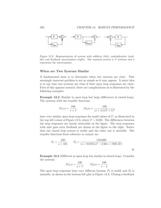
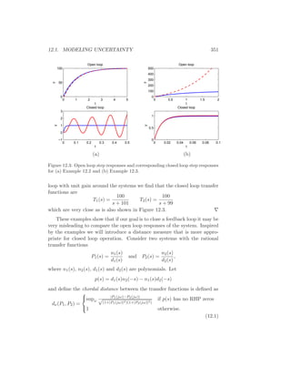
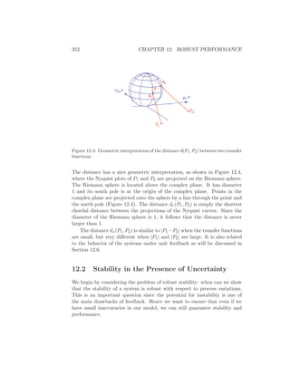
388. 376 CHAPTER 12. ROBUST PERFORMANCE
Robustness
There are strong robustness results associated with the H∞ controller. We
can understand this intuitively by comparing Equations (12.1) and (12.18).
We can then conclude that
H(P, C) ∞ =
1
d(P, −1/C)
(12.20)
The inverse of H(P, C) ∞ is thus equal to chordal distance between P and
1/C. If we find a controller C with H(P, C) ∞ < γ this controller will
then stabilize any process P∗ such that d(P, P∗) < γ.
Limits of Robust Design
There is a limit to what can be achieved by robust design. In spite of the nice
properties of feedback there are situations where the process variations are
so large that it is not possible to find a linear controller which gives a robust
system with good performance. It is then necessary to use other controllers.
In some cases it is possible to measure a variable that is well correlated
with the process variations. Controllers for different parameters values can
then be designed and the corresponding controller can be chosen based on
the measured signal. This type of controller is called gain scheduling. The
cruise controller is a typical example where the measured signal could be
gear position and velocity. Gain scheduling is the common solution for high
performance aircraft where scheduling is done based on Mach number and
dynamic pressure. When using gain scheduling it is important to make sure
that switches between the controllers do not create undesirable transients.
If it is not possible to measure variables related to the parameters, it is
possible to use automatic tuning and adaptive control. In automatic tuning
process dynamics is measured by perturbing the system and a controller
is then designed automatically. Automatic tuning requires that parameters
remain constant, it has been widely applied for PID control, it is a reasonable
guess that, in the future, many controllers will have features for automatic
tuning. If parameters are changing it is possible to use adaptive methods
where where process dynamics is measured on-line.
12.7 Further Reading
Robustness was a central issue in classical control, see [Bod45]. It was
deemphasized in the euphoria of the development of design methods based

389. 12.8. EXERCISES 377
on optimization. The strong robustness of LQ control based on state feed-
back shown by Anderson and Moore [?] contributed to the optimism. The
poor robustness of output feedback based on LQG was pointed out by Rosen-
brock [RM71], Horowitz [Hor75] and Doyle [Doy78] resulted in a renewed
interest in robustness. A major step forward was the development of design
methods where robustness was explicitly taken into account. Seminal work
by Zames [Zam81] was a major step forward. Robust control was origi-
nally developed using powerful results from the theory of complex variables
which unfortunately gave controllers of very high order. A major break
through was given by Doyle, Glover, Khargonekar, and Francis [DGKF89]
who showed that the solution could be obtained using Riccati equations and
that a controller of low order could be found. This paper led to an exten-
sive treatment of the so-called H∞ control [Fra87, MG90, DFT92, GL95,
ZDG96, SP96, Vin01]. A major advantage of the theory is that it combines
much of the intuition from servomechanism theory with sound numerical
algorithms based on numerical linear algebra and optimization. The results
have been extended to nonlinear systems by treating the design problem as
a game where the disturbances are generated by an adversary as described
in [BB91]. Auto-tuning and adaptive control are treated in [˚AW95] and
automatic tuning is dealt with in depth in [˚AH05].
12.8 Exercises
1. Show that an additive disturbance δadd, show that it can create RHP
zeros, but not RHP poles, and that a feedback disturbance δfbk can
create RHP poles but not RHP zeros. Also give constructive examples.
2. Compute the distance between the systems
P1(s) =
k
s + 1
, andP2(s) =
k
s − 11
.
for k = 1, 2 and 5.
3. The distance measure is closely related to closed loop systems with
unit feedback. Show how the measure can be modified to applied to
an arbitrary feedback.
4. Consider the Nyquist curve in Figure 12.12. Explain why part of the
curve is approximately a circle. Derive a formula for the center and
the radius and compare with the actual Nyquist curve.

390. 378 CHAPTER 12. ROBUST PERFORMANCE
5. Consider the transfer functions in examples 12.2 and 12.3. Compute
the distance measure δ(P1, P1) in both cases. Repeat the calculations
when the controller is C = 0.1.
6. (Ideal Delay Compensator) Consider a process whose dynamics is a
pure time delay, the transfer function is P(s) = e−s. The ideal delay
compensator is a controller with the transfer function C(s) = 1/(1 −
e−s). Show that the sensitivity functions are T(s) = e−s and S(s) =
1 − e−s and that the closed loop system will be unstable for arbitrary
small changes in the delay.
7. Let P and C be matrices whose entries are complex numbers, show
that the singular values of the matrix
H(P, C) =


1
1 + PC
P
1 + PC
C
1 + PC
PC
1 + PC


are σ1 = 0 and σ2 = supω
(1 + |P(jω)|2)(1 + |C(jω)|2)
|1 + P(jω)C(jω)
.
8. Show that
sup
w
|1 + P(jω)C(jω)|
(1 + |P(jω)|2)(1 + |C(jω)|2)
= d(P, −1/C)

391. Bibliography
[Abk69] M. A. Abkowitz. Stability and Motion Control of Ocean Vehicles. MIT
Press, Cambridge, MA, 1969.
[˚AH95] K. J. ˚Astr¨om and T. H¨agglund. PID Controllers; Theory, Design and
Tuning. Instrument Society of American, 1995.
[˚AH05] Karl Johan ˚Astr¨om and Tore H¨agglund. Advanced PID Control. ISA
- The Instrumentation, Systems, and Automation Society, Research
Triangle Park, NC 27709, 2005.
[˚AKL05] K. J. ˚Astr¨om, R. E. Klein, and A. Lennartsson. Bicycle dynamics and
control. IEEE Control Systems Magazine, 25(4):26–47, 2005.
[˚Ang61] A. I. ˚Angstr¨om. Neue Methode, das v¨armeleitungsverm¨ogen der K¨orper
zu bestimmen. Ann. der Physik und Chemie, 114:513–530, 1861.
[˚Ast70] K. J. ˚Astr¨om. Introduction to Stochastic Control Theory. Academic
Press, 1970. Republished by Dover Publications, 2006.
[˚AW95] K. J. ˚Astr¨om and B. Wittenmark. Adaptive Control. Addison-Wesley,
Reading, Massachusetts, second edition, 1995.
[B˚A70] R. Bellman and K. J. ˚Astr¨om. On structural identifiability. Mathemat-
ical Biosciences, 7:329–339, 1970.
[BB91] T. Basar and P. Bernhard. H∞
-Optimal control and related minimax
design problems - A Dynamic game approach. Birkhauser, Boston, 1991.
[Bec05] J. Bechhoefer. Feedback for physicists: A tutorial essay on control.
Reviews of Modern Physics, 77:783–836, 2005.
[Ben86a] S. Bennett. A History of Control Engineering: 1800–1930. Peter Pere-
grinus, 1986.
[Ben86b] S. Bennett. A History of Control Engineering: 1930–1955. Peter Pere-
grinus, 1986.
[Ber54] L. L. Beranek. Acoustics. McGraw-Hill, New York, NY, 1954.
[BK64] R. E. Bellman and R. Kalaba. Selected Papers on Mathematical Trends
in Control Theory. Dover, New York, NY, 1964.
379

392. 380 BIBLIOGRAPHY
[Bla34] H. S. Black. Stabilized feedback amplifiers. Bell System Technical Jour-
nal, 13:1–2, 1934.
[Bla91] J. H. Blakelock. Automatic Control of Aircraft and Missiles. Addison-
Wesley, Cambridge, MA, second edition, 1991.
[Bod45] H. W. Bode. Network Analaysis and Feedback Amplifier Design. Van
Nostrand, 1945.
[Bod60] H. W. Bode. Feedback—The History of an Idea. In Symposium on Ac-
tive Networks and Feedback Systems. Polytechnic Institute of Brooklyn,
1960. in [BK64].
[BP96] M. B. Barron and W. F. Powers. The role of electronic controls for future
automotive mechatronic systems. IEEE Transactions on Mechatronics,
1(1):80–89, 1996.
[Bro00] R. W. Brockett. New issues in the mathematics of control. In B. En-
gquist and W. Schmid, editors, Mathematics Unlimited—2001 and Be-
yond, pages 189–220. Springer Verlag, 2000.
[BS60] J. F. andG. Reethof Blackburn and J.L. Shearer. Fluid Power Control.
MIT Press, Cambridge, MA, 1960.
[Can03] R. H. Cannon. Dynamics of Physical Systems. Dover, originally pub-
lished by mc-graw hill 1967 edition, 2003.
[CD75] R. F. Coughlin and F. F. Driscoll. Operational Amplifiers and Linear
Integrated Circuits. 6th Edition. Prentice Hall, Englewood Cliffs, NJ,
1975.
[CD91] F. M. Callier and C. A. Desoer. Linear System Theory. Springer-Verlag,
1991.
[CJ59] H. S. Carslaw and J. C. Jaeger. Conduction of Heat in Solids. Carendon
Press, Oxford, second edition, 1959.
[DB04] R. C. Dorf and R. H. Bishop. Modern Control Systems. Prentice Hall,
tenth edition, 2004.
[DFT92] J. C. Doyle, B. A. Francis, and A. R. Tannenbaum. Feedback Control
Theory. Macmillan Publishing Company, 1992.
[DGKF89] J. C. Doyle, K. Glover, P. P. Khargonekar, and B. A. Francis. State-
space solutions to standard H2 and H∞ control problems. IEEE Trans-
actions on Automatic Control, 34(8):831–847, 1989.
[DH85] J.P. Den Hartog. Mechanical Vibrations. Dover, New York, 1985.
Reprint of fourth edition from 1956, first edition published in 1934.
[dJ02] H. de Jong. Modeling and simulation of genetic regulatory systems: A
literature review. Journal of Computational Biology, 9:67–103, 2002.

393. BIBLIOGRAPHY 381
[DM02] L. Desbourough and R. Miller. Increasing customer value of indus-
trial control performance monitoring - Honeywell’s experience. In Sixth
International Conference on Chemical Process Control. AIChE Sympo-
sium Series Number 326 (Volume 98), 2002.
[Dos68] F.H. Dost. Grundlagen der Pharmakokinetik. Thieme Verlag, Stuttgart,
1968.
[Doy78] J. C. Doyle. Guaranteed margins for lqg regulators. IEEE Transactions
on Automatic Control, 23(4):756–757, 1978.
[Dys04] F. Dyson. A meeting with enrico fermi. Nature, 247(6972):297, 2004.
[EG05] S. P. Ellner and J. Guckenheimer. Dynamic Models in Biology. Prince-
ton University Press, 2005.
[EL00] M. B. Elowitz and S. Leibler. A synthetic oscillatory network of tran-
scriptional regulators. Nature, 403(6767):335–338, 2000.
[Ell94] J. R. Ellis. Vehicle Handling Dynamics. Mechanical Engineering Pub-
lications, London, 1994.
[Fey70] R. P. Feynmann. Lectures on Physics. Addison Wesley, New York, NY,
1970.
[Fou07] J. B. J. Fourier. On the Propagation of Heat in Solid Bodies. 1807.
[FPEN05] G. F. Franklin, J. D. Powell, and A. Emami-Naeini. Feedback Control
of Dynamic Systems. Addison Wesley Longman, fifth edition, 2005.
[Fra87] B. A. Francis. A Course in H∞ Control. Springer-Verlag, Berlin, 1987.
[Fri04] B. Friedland. Control System Design: An Introduction to State Space
Methods. Dover, 2004.
[GB42] M. A. Gardner and J. L. Barnes. Transients in Linear Systems. John
Wiley, New York, 1942.
[GF71] L. Gunkel and G. F. Franklin. A general solution for linear sampled
data systems. IEEE Transactions on Automatic Control, AC-16:767–
775, 1971.
[GH83] J. Guckenheimer and P. Holmes. Nonlinear Oscillations, Dynamical
Systems, and Bifurcations of Vector Fields. Springer Verlag, 1983.
[Gil63] E. Gilbert. Controllability and observability in multivariable control
systems. SIAM J. Control, 1(1):128–151, 1963.
[GL95] Michael Green and D. J. N. Limebeer. Linear Robust Control. Prentice
Hall, Englewood Cliffs, N.J., 1995.
[God83] K. Godfrey. Compartment models and their application. Academic
Press, New York, NY, 1983.

394. 382 BIBLIOGRAPHY
[Gol53] H. Goldstein. Classical Mechanics. Addison-Wesley, Cambridge, MA,
1953.
[Gol70] S. W. Golomb. Mathematical models—uses and limitations. Simulation,
4(14):197–198, 1970.
[GP82] M. Giobaldi and D. Perrier. Pharmacokinetics, Second Edition. Marcel
Dekker, New York, 1982.
[Gui63] E. A. Guillemin. Theory of Linear Physical Systems. MIT Press, Cam-
bridge, MA, 1963.
[HB90] J. K. Hedrick and T. Batsuen. Invariant properties of automobile sus-
pensions. In Proc. Institution of Mechanical Engineers, volume 204,
pages 21–27, London, UK., 1990.
[HD95] M. B. Hoagland and B. Dodson. The Way Life Works. Times Books,
1995.
[HDPT04] J. L. Hellerstein, Y. Diao, S. Parekh, and D. M. Tilbury. Feedback
Control of Computing Systems. John Wiley, New York, 2004.
[Hen06] Dan Henriksson. Resource-Constrained Embedded Control and Com-
puting Systems. PhD thesis, Department of Automatic Control, Lund
Institute of Technology, Sweden, January 2006.
[Her04] David V. Herlihy. Bicycle - The History. Yale University Press, Yale,
NH, 2004.
[HH52] A. L. Hodgkin and A. F. Huxley. A quantitative description of mem-
brane current and its application to conduction and excitation in nerve.
Journal of Physiology, 117(500–544), 1952.
[HLA04] D. Henriksson, Y. Lu, and T. Abdelzaher. Improved prediction for
web server delay control. In 16th Euromicro Conference on Real-Time
Systems, Catania, Sicily, Italia, 2004.
[Hor75] I. M. Horowitz. Superiority of transfer function over state-varible meth-
ods in linear, time-invariant feedback system design. IEEE Transactions
on Automatic Control, AC-20(1):84–97, 1975.
[HW00] D. Hanahan and R. A. Weinberg. The hallmarks of cancer. Cell, 100:57–
70, 2000.
[Isi89] A. Isidori. Nonlinear Control Systems. Springer-Verlag, 2nd edition,
1989.
[Jac72] J. A. Jacquez. Compartment analysis in biology and medicine. Elsevier,
Amsterdam, 1972.
[Jac88] V. Jacobson. Congestion avoidance and control. In Proc. SIGCOMM
’88, pages 314–329, 1988.

395. BIBLIOGRAPHY 383
[JNP47] H. James, N. Nichols, and R. Philips. Theory of Servomechanisms.
McGraw-Hill, 1947.
[JT61] P. D. Joseph and J. T. Tou. On linear control theory. Transactions of
AIEE, 80(18), 1961.
[Jun02] W. G. (editor) Jung, editor. Op Amp Applications. Analog Devices,
Norwood, MA, 2002.
[Kal60] R. E. Kalman. Contributions to the theory of optimal control. Boletin
de la Sociedad Mat´ematica Mexicana, 5:102–119, 1960.
[Kal61a] R. E. Kalman. New methods and results in linear prediction and filter-
ing theory. Technical Report 61-1, RIAS, February 1961. 135 pp.
[Kal61b] R. E. Kalman. On the general theory of control systems. In Proceedings
first IFAC Congress on Automatic Control, Moscow, 1960, volume 1,
pages 481–492, London, 1961. Butterworths.
[KB61] R. E. Kalman and R. S. Bucy. New results in linear filtering and predic-
tion theory. Trans ASME (J. Basic Engineering), 83 D:95–108, 1961.
[Kel85] F. P. Kelley. Stochastic models of computer communication. J. Royal
Statistical Society, B47(3):379–395, 1985.
[Kel94] K. Kelly. Out of Control. Addison-Wesley, 1994. Available at http:
//www.kk.org/outofcontrol.
[KFA69] R. E. Kalman, P. L. Falb, and M. A. Arbib. Topics in Mathematical
System Theory. McGraw-Hill, 1969.
[KG02] B. C. Kuo and F. Golnaraghi. Automatic Control Systems. Wiley,
eighth edition, 2002.
[Kha92] H. K. Khalil. Nonlinear Systems. Macmillan Publishing Company, 1992.
[KHN63] R. E. Kalman, Y. Ho, and K. S. Narendra. Controllability of Linear Dy-
namical Systems, volume 1 of Contributions to Differential Equations.
John Wiley & Sons, Inc., New York, 1963.
[Kit95] C. Kittel. Introduction to Solid State Physics. John Wiley, New York,
1995.
[KN00] U. Kiencke and L. Nielsen. Automotive Control Systems : For Engine,
Driveline, and Vehicle. Springer, Berlin, 2000.
[Kum01] P. R. Kumar. New technological vistas for systems and control: The
example of wireless networks. Control Systems Magazine, 21(1):24–37,
2001.
[LA96] D. C. Liaw and E. H. Abed. Control of compressor stall inception: A
bifurcation-theoretic approach. Automatica, 32(1):109–115, 1996.

396. 384 BIBLIOGRAPHY
[Lue71] D. G. Luenberger. An introduction to observers. IEEE Transactions
on Automatic Control, 5(10):213–214, 1971.
[Lun05] K. H. Lundberg. History of analog computing. IEEE Control Systems
Magazine, 25(3):22–28, 2005.
[Mac37] D. A. MacLulich. Fluctuations in the numbers of the varying hare (Le-
pus americanus). University of Toronto Press, 1937.
[Man02] R. Mancini. Op Amps for Everyone. Texas Instruments, Houston. TX,
2002.
[May70] O. Mayr. The Origins of Feedback Control. MIT Press, 1970.
[McF53] M. W. McFarland, editor. The Papers of Wilbur and Orville Wright.
McGraw Hill, 1953.
[MG90] D. C. MacFarlane and K. Glover. Robust controller design using nor-
malized coprime factor plant descriptions. Springer, New York, 1990.
[Mil66] H. T. Milhorn. The Application of Control Theory to Physiological
Systems. Saunders, 1966.
[Min02] D. A. Mindel. Between Human and Machine: Feedback, Control, and
Computing Before Cybernetics. Johns Hopkins University Press, 2002.
[MR94] J. E. Marsden and T. S. Ratiu. Introduction to Mechanics and Symme-
try. Springer Verlag, 1994.
[MS93] L. Moore and D. Smith. Predator-prey models, 1993. http://www.
math.duke.edu/education/ccp.
[Mur03] R. M. Murray, editor. Control in an Information Rich World: Report
of the Panel on Future Direcitons in Control, Dynamics and Systems.
SIAM, 2003. Available at http://www.cds.caltech.edu/∼murray/
cdspanel.
[Mur04] J. D. Murray. Mathematical Biology, volume I and II. Springer, third
edition, 2004.
[NS99] H. Nijmeijer and J. M. Schumacher. Four decades of mathematical
system theory. In J. W. Polderman and H. L. Trentelman, editors,
The Mathematics of Systems and Control: From Intelligent Control to
Behavioral Systems, pages 73–83. Univ. of Groningen, 1999.
[Nyq32] H. Nyquist. Regeneration theory. Bell System Technical Journal,
11:126–147, 1932.
[Oga01] K. Ogata. Modern Control Engineering. Prentice-Hall, fourth edition
edition, 2001.
[Phi48] G. A. Philbrick. Designing industrial controllers by analog. Electronics,
21(6):108–111, 1948.

397. BIBLIOGRAPHY 385
[Pit99] J. Pitman. Probability. Springer, 1999.
[PPP02] S. Prajna, A. Papachristodoulou, and P. A. Parrilo. SOSTOOLS: Sum
of squares optimization toolbox for MATLAB, 2002. Available from
http://www.cds.caltech.edu/sostools.
[RM71] H. H. Rosenbrock and P. D. Moran. Good, bad or optimal? IEEE
Transactions on Automatic Control, AC-16(6):552–554, 1971.
[Row58] F. Rowsone Jr. What it’s like to drive an auto-pilot car. Popular
Science Monthly, April 1958. Available at http://www.imperialclub.
com/ImFormativeArticles/1958AutoPilot.
[Sar91] D Sarid. Atomic Force Microscopy. Oxford University Press, Oxford,
1991.
[Sch01] G. Schitter. High performance feedback for fast scanning atomic force
microscopes. Review of Scientific Instruments, 72(8):3320–3327, 2001.
[SEM03] D. E. Seborg, T. F. Edgar, and D. A. Mellichamp. Process Dynamics
and Control. Wiley, 2003.
[Sen01] S. D. Senturia. Microsystem Design. Kluwer, Boston, MA, 2001.
[She62] C. W. Sheppard. Basic Principles of the Tracer Method. John Wiley &
Sons, Inc., New York,, 1962.
[SP96] S Skogestad and I. Postlethwaite. Multivariable feedback control: anal-
ysis and design. Wiley, Chichester, UK, 1996.
[Sta59] L. Stark. Oscillations and noise in the human pupil servomechanism.
Proceedings of the Institute of Radio Engineers, IRE-47:1925–1939,
1959.
[Sta68] L. Stark. Neurological Control Systems - Studies in Bioengineering.
Plenum Press, New York, N. Y., 1968.
[Sto94] S. H. Storgatz. Nonlinear Dynamics and Chaos, with Applications to
Physics, Biology, Chemistry, and Engineering. Addison-Wesley, 1994.
[Str88] G. Strang. Linear Algebra and its Applications. Harcourt Brace Jo-
vanovich, San Diego, third edition, 1988.
[Teo37] T. Teorell. Kinetics of distribution of substances administered to the
body i and ii. Archives Internationales de Pharmacodynamie et de Ther-
apie, 57:205–240, 1937.
[Til01] M. Tiller, editor. Introduction to Physical Modeling with Modelica.
Springer, 20001.
[Tsi54] H. S. Tsien. Engineering Cybernetics. McGraw-Hill, 1954.
[Vin01] G. Vinnicombe. Uncertainty and Feedback: H∞ loop-shaping and the
ν-gap metric. Imperial College Press, London, 2001.

398. 386 BIBLIOGRAPHY
[Whi99] F. J. W. Whipple. The stability of the motion of a bicycle. Quarterly
Journal of Pure and Applied Math., 30:312–348, 1899.
[Wie48] N. Wiener. Cybernetics: Or Control and Communication in the Animal
and the Machine. John Wiley, 1948.
[Wig90] S. Wiggins. Introduction to Applied Nonlinear Dynamical Systems and
Chaos. Springer-Verlag, 1990.
[Wil99] H. R. Wilson. Spikes, Decisions, and Actions: The Dynamical Founda-
tions of Neuroscience. Oxford University Press, 1999.
[Wil04] D. G. Wilson. Bicycling Science. MIT Press, Cambridge, MA, 2004.
Third edition, with contributions by Jim Papadopoulos.
[WT24] E. P. M. Widmark and J. Tandberg. ¨Uber die bedinungen fr die akku-
mulation indifferenter narkotika. Biochemische Zeitung, 148:358–389,
1924.
[Zam81] G. Zames. Feedback and optimal sensitivity: Model reference transfor-
mations, multiplicative seminorms, and approximative inverse. IEEE
Transactions on Automatic Control, AC-26(2):301–320, 1981.
[ZDG96] J. C. Zhou, J. C. Doyle, and K. Glover. Robust and optimal control.
Prentice Hall, New Jersey, 1996.

399. Index
A/D converters, see analog-to-digital con-
verters
active filter, 163, 171
actuation, 4, 5
Adams (modeling tool), 59
adaptive control, 376, 377
adaptive optics, 15
additive uncertainty, 349
adjacency matrix, 69
aerospace systems, 8
airspace management, 9
analog-to-digital converters, 5, 63, 318
zz, see also delta-sigma converters
anti-windup, 314
argument, 260
asymptotic stability, 123
atomic force microscope, 95–99, 265
attractor, 124
autocoding, 30
automatic reset, 304
automatic tuning, 376, 377
automobiles, 7, 24, 60, 82, 91
zz, see also cruise control, vehicle steer-
ing
autonomous system, 37
zz, see also time-invariant systems
autonomous vehicles, 22–23
autopilot, 21
AUTOSIM (modeling tool), 59
balance system, 44, 114
reachability, 191
Bell Labs, 20, 299
Bennett, S., 31
bicycle dynamics, 83–85, 218
bifurcation, 138
bifurcation control, 140
bifurcation diagram, 139
biological engineering, 4
biological systems, 1
repressilator, 72–73
zz, see also drug administration, pop-
ulation dynamics
black box models, 34
Black, H. S., 20, 22, 63, 85, 88, 144, 347
block diagrams, 55
Bode plot, 259, 260
Bode’s integral formula, 363
Bode’s relations, 292
Brockett, R. W., x, 1
calibration, 202
carrying capacity, 103
center, 124
centrifugal governor, 2, 6
chain of integrators, 76
chemical industry, 12
chordal distance, 351
circular reasoning, 84
closed loop, 2, 4, 7, 182, 278
versus open loop, 2, 279, 299, 323
command and control, 9
compartment models, 99
complementary sensitivity function, 326, 361
complexity
of control systems, 24
component failures, robustness to, 4
computation, 5
computed torque, 183
computer numerically controlled (CNC) ma-
chining, 8
computer science
relationship to control, 6
conditional stability, 287
congestion control, 9, 66, 125, 132
consensus, 68
consumer electronics, 3
control, 4–6
387

400. 388 INDEX
as enabling technology, 8
early examples, 7
modeling, 39–40
of bifurcations, 140
successes of, 31
synthesis, 30
system, 4
control error, 25
control law, 5, 25, 197
control matrix, 43, 47
controlled differential equation, 37
convolution equation, 156
critical point, 279
critically damped, 173
crossover frequency inequality, 342
cruise control, 6, 7, 77–82, 141, 177, 181,
210, 281, 311, 313, 314, 348, 355
cybernetics, 11
D/A converters, see digital-to-analog con-
verters
damped oscillator, 112
damping factor, 172
DARPA Grand Challenge, 22
DC gain, see zero frequency gain
declarative description, 41
delay control, 93
delay margin, 289
delta function, see impulse
delta-sigma converters, 63
derivative action, 305
derivative gain, 302
derivative time constant, 302
design of dynamics, 20
diagonal system, 153
difference equations, 46–49
differential algebraic equations, 41
differential equations, 35, 111–117
finite escape time, 116
non-unique solutions, 116
solution, 112, 151
digital-to-analog converters, 5
direct term, 43, 47
discrete time systems, 46
disturbance rejection, 4, 6
disturbances, 5, 29, 40
Dodson, B., 1
double integrator, 151, 188
Doyle, J. C., x, 215, 345, 377
drug administration, 99–102, 207
drugadministration
zz, see also compartment models
dual, 219
duality, 224
ducted fan
pitch control, 338
dynamic compensator, 210
dynamic inversion, 183
dynamical system, 33
dynamics, 4, 7
dynamics matrix, 43, 47, 130, 153
economic systems, 18, 24
ecosystems, 4, 17
eigenvalue assignment, 202, 222, 227
eigenvalues, 131, 161
electrical engineering, 37–38
electronic amplifiers, 4, 34
emissions control, 7
energy systems, 18
entertainment robots, 11
environmental science, 4, 13, 18
equilibrium point, 103, 119
stability, 122
error feedback, 316, 325
exponential signals, 243
exponential stability, 142
extended Kalman filter, 235
external descriptions, 34
external disturbances, 5
feedback, 1–4, 7, 20
as technology enabler, 3
drawbacks, 23
in biological systems, 1, 2, 16–17
zz, see also biological systems
in ecological systems, 17
in engineered systems, see control
in financial systems, 4
in nature, 15–18
loop, 4
positive, see positive feedback
versus control, 4
feedback linearizable, 182
feedback loop, 4
feedforward, 24
financial systems, 18
finite escape time, 116

401. INDEX 389
first order system, 309
flight control, 20, see also vectored thrust
aircraft
flow, 36
flow model, 90
flyball governor, see centrifugal governor
forced response, 29
frequency response, 38, 52
fully actuated, 252
fundamental limitations, 363
gain, 170, 296–299
zero frequency, see zero frequency gain
zz, see also loop gain
gain crossover frequency, 289, 329
gain margin, 288, 289, 329
gain scheduling, 94, 235, 376
Gang of Four, 326
Gang of Six, 325
gene regulation, 16
global climate, see environmental science
glucose regulation, 2, 99
Harrier AV-8B aircraft, 61
heat propagation, 74, 250, 275, 281
Heaviside, 183
high frequency roll off, 360
higher levels of decision making, 9, 22
Hoagland, M. B., 1
Hodgkin-Huxley equations, 73
homeostasis, see biological systems
homogeneous solution, 147, 251
Honeywell, 6
identification, see system identification
imperative description, 41
impulse, 157
impulse response, 149, 157, 158
information science, 4
information systems, 9
input, 37
input sensitivity function, 326
input/output models, 5, 28, 34
instability, 23
instrumentation, 14
insulin, see glucose regulation
integral action, 7, 202, 304
integral control, 27
integral gain, 302, 360
integral time constant, 302
integral windup, 301
integrator windup, 233, 313, 315
intelligent machines, see robotics
interconnection, 5
internal descriptions, 34
internal model principle, 228, 236
Internet, 4, 9
Internet Protocol (IP), 66
intial value problem, 112
invariant (programming), 70
invariant set, 135
inverse response, 295
inverted pendulum, 46, 119
damped, 124
linear approximation, 126
Jacobian linearization, 179
Jordan decomposition, 164
Jordan form, 163
trivial block, 164
Josephson Junction, 64
josephson junction, 64
Kalman decomposition, 272
Kalman, R. E., 187
Kelly, K., 31
Krasovskii-Lasalle principle, 134–136
LabVIEW, vii, 59, 114
Laplace transform, 268–271
Laplace transforms, ix
Laplacian matrix, 70
Lasalle’s invariance principle, see Krasovskii-
Lasalle principle
lead compensator, 338
limit cycle, 120
linear input/output system, 145
linear quadratic control, 372
linear system, 43
linear systems, 38
linearization, 176–183
Lipschitz continuity, 117
load disturbance, 324
load sensitivity function, 326
logistic growth model, 103
loop gain, 279
loop shaping, 334
loop transfer function, 278

402. 390 INDEX
LQ control, 372
LTI systems, 147
Lyapunov equation, 131
Lyapunov function, 128, 129
Lyapunov stability theorem, 128
manufacturing, 8
manufacturing systems, 18
Mars Exploratory Rovers, 11
materials science, 12
Mathematica, 30, 114
MATLAB, vii, 30, 32, 58, 114, 115, 118, 164,
180, 203, 212, 226, 231, 374
matrix exponential, 150–153
maximum complementary sensitivity, 330
maximum sensitivity, 329
Mayr, O., 31
measurement noise, 324
measures, 29
mechanical systems, 182
mechanics, 34–37
microsystems, 12
Mindell, D., 31
minimum phase, 293
modal form, 159, 160
mode, 154, 155, 251
mode shape, 154
mode: Jordan form, 165
model, 33
model reduction, 5, 29
model uncertainty, 355
Modelica, 42, 59
modeling, 5, 12, 28
modeling from experiments, 53
nanotechnology, 12
negative definite, 128, 131
negative feedback, 20
networks, 9
neuroscience, 73
neutrally stable, 122
noise, 229
noise sensitivity function, 326
non-minimum phase, 293
non-unique solutions, 116
normalization, 181
Nyquist criterion, 280, 285
Nyquist curve, 279
Nyquist plot, 279
observability, 40, 216
rank condition, 217
Observable Canonical Form, 219
observable canonical form, 219
observers, 215
Octave, 114
ODEs, see differential equations
ω limit set, 134
on-off control, 25
open loop, 2, 189
operational amplifier, 85–89, 248
operational amplifier (op amp), 85
order, 42
order of a system, 43
ordinary differential equation: controlled,
37
ordinary differential equations, see differen-
tial equations, 42–46
output sensitivity function, 326
overdamped, 173
overshoot, 168
overshoot: error feedback, 331
parametric stability diagram, 139
parametric uncertainty, 347
particular solution, 147
passivity theorem, 299
pharmacokinetics, see drug administration
phase, 170
minimum vs. nonminimum, 293
phase crossover frequency, 288
phase margin, 289, 329
phase portrait, 117
physics
relationship to control, 5
PI control, 27
PI control, first order systems, 309
PID control, 27
PID controller, 340
pitchfork bifurcation, 138, 141
pole, 251
right half plane, 343, 344
pole zero diagram, 252
pollution, 7
population dynamics, 102–107
positive definite, 128, 131
positive feedback, 25
positive real, 363
positive semidefinite, 128

403. INDEX 391
predator prey system, 47, 103, 120, 139, 204
prediction, ability of controllers, 27
principle of the variation of the argument,
283
process control, 8, 12, 25, 29
proportional control, 26
zz, see also PID control
proportional gain, 302
proportional, integral, derivative control, see
PID control
protocols, 4
public awareness, 7
pupil response, 266, 291
pure error feedback, 325
pure exponential response, 245
Q-value, 174, 263
quantum systems, 17
quarter car model, 273
random variable, 90
reachability, 39, 188
rank condition, 190
reachability matrix, 190
reachable canonical form, 193, 196, 200
real-time systems, 6
receding horizon control, 94
reference weighting, 316
reference weights, 316
region of attraction, 136
regulation, 1
relay feedback, 308
reliability, 7
repressilator, 72–73
reset, 304
resource management, 18
Riccati equation, 212, 374
rise time, 168
robotics, 4, 11–12
robustness, 19–20, 29
rush-hour effect, 91
saddle, 124
saturation function, 86
SBML (Systems Biology Markup Language),
59
Scilab, 114
second order system, 35
second order systems, 172
sensing, 4, 5
sensitivity crossover frequency, 330
sensitivity function, 326
sensitivity function:disturbance attenuation,
360
sensor matrix, 43, 47
sensors, 13
separation principle, 228
setpoint, 302, 316
setpoint weights, 316
settling time, 168
Sigma-delta converters, see delta-sigma con-
verters
simple models, 356
simulation, 49
SIMULINK, 58, 59, 180
sink, 124
small gain theorem, 298–299, 356–357
Sony AIBO, 11
source, 124
spectrum analyzer, 265
Sperry autopilot, 21
SPICE (modeling tool), 59
spring mass system, 49, 135, 160, 174
system identification, 54
stability, 4, 5, 20, 29, 51, 122–136
exponential, 142
linear system, 162
local versus global, 123, 136, 137, 183
stability by linearization, 183
stability margin, 289
stability margins, 288
stable, 49
state, 35, 42
state estimators, see oservers215
state models, 34
state space, 35, 42–55
state space model, 42
state vector, 42
steady state
value, 168
steady state gain, see zero frequency gain
steady state response, 50
steam engine, 3
Stein, G., x, 1
step input, 166
step response, 38, 149, 158, 166
subcritical bifurcation, 138
supercritical bifurcation, 138

404. 392 INDEX
superposition, 145
supply chains, 18
supremum (sup), 297
system identification, 28
system: time-invariant, 43
temperature control, 1, 7
thermostat, 6, 7
time constant, 184
time delay, 7, 9, 293, 343
time invariance, 147
time-invariant system, 42
time-invariant systems, 38
traffic management, 9
trail, 84
transcriptional regulation, 71
transfer function, 241, 245, 247
transfer function: differentiator, 247
transfer function: integrator, 247
transient, 188
Transmission Control Protocol (TCP), 66
transportation systems, 8
Tsien, H. S., 11
two degrees of freedom, 234
uncertainty, 5, 19–20, 40, 347–352
component or parameter variation, 5
unmodeled dynamics, 5, 349
undamped oscillator, 152
underdamped, 113, 173
unit step, 166
unmodeled dynamics, 30, 349
unobservable systems, 219
unreachable system, 200
unstable, 123
unstable pole/zero cancellation, 259
vector field, 36
vectored thrust aircraft, 61
vehicle steering, 60, 180, 198, 225, 229, 256,
290, 296
lack of robustness, 366
vertical takeoff and landing, see vectored
thrust aircraft
vibration absorber, 274
waterbed effect, 363, 364
Watt governor, see centrifugal governor
web server admission control, 89–95
web site, vii
white box, 34
Wiener, N., 11
winding number, 283
windup, see integrator windup
Wright brothers, 20
Youla parameterization, 357, 358
zero, 251
right half plane, 344
zero frequency gain, 171, 198, 202, 251, 303,
307, 329
zeros, signal blocking property, 251
Ziegler-Nichols methods, 306