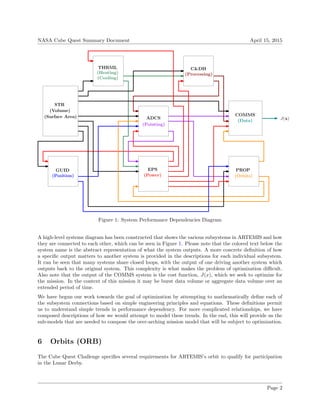
This document is a final report for the Advanced Radio Transmission Experimental Michigan Satellite (ARTEMIS) project. It provides an overview of the mission requirements and design drivers for the subsystems of the ARTEMIS CubeSat. The report describes the preliminary analyses and simulation tools used to evaluate the performance of the satellite's orbits, communication system, propulsion system, electrical power system, attitude determination and control system, command and data handling system, structures, thermal control system, and guidance system.
![NASA Cube Quest Summary Document April 15, 2015
6.1 ORB Performance Dependencies
The primary performance dependencies for the ORB subsystem are launch selection and the onboard propul-
sion unit. These constrain the trajectories available to ARTEMIS.
6.1.1 Launch Selection
The Cube Quest Challenge Lunar Derby competition time is defined as the 365 day period which begins
with the launch of the EM-1 mission. NASA has offered the five teams who score the highest in Ground
Tournament 4 the opportunity to be carried aboard the EM-1 mission, currently scheduled for launch in
December 2018. As EM-1 approaches the Moon, it will release secondary payloads (including the selected
Cube Quest competitors) at a specified range in its orbit. NASA provided the expected payload disposal
trajectory for the original launch date [1], specified in Table 1; an updated trajectory remains forthcoming.
Although maneuvering from EM-1 to Low Lunar Orbit (LLO) is likely the quickest option, more frequent,
earlier launches are available to Low Earth Orbit (LEO), a Geosynchronous Transfer Orbit (GTO), and
Geosynchronous Earth Orbit (GEO). These launches may offer simpler trajectories, and therefore simpler
mission planning. Preliminary analysis, covered in Section 6.2, indicates that a low-thrust transfer from
LEO to LLO, while possible, would require upwards of 7 km/s total ∆V and over a year to complete [2].
Therefore, we have chosen to focus on transfers from GEO to LLO or EM-1 to LLO. Spaceflight Services
provides three such launch opportunities for a 6U Cubesat to GTO, one each in 2015, 2016, and 2017 [3].
Table 1: EM-1 Payload Disposal Trajectory. Coordinates are with respect to J2000 inertial reference frame.
State Value Units
Rx -1.5015e+04 km
Ry -2.3569e+04 km
Rz 2.2415e+03 km
Vx -4.8554e−01 km/s
Vy -5.0488e+00 km/s
Vz -8.7999e−01 km/s
Epoch 15 Dec 2017 14:56:42.2 Barycentric Dynamical Time
6.1.2 Propulsion System
Propulsion systems fall into two broad categories: high thrust/low specific-impulse chemical propulsion,
and low thrust/high specific-impulse electric propulsion. Chemical propulsion enables lunar orbit insertion
within a week in most cases, at the cost of higher propellant mass but lower power consumption than an
electric propulsion system. Lunar orbit maneuvers using an electric propulsion systems have flight times
on the order of six to eight months but require far less propellant mass than a chemical thruster, however
they also consume much more power due to the long-duration continuous burns required. Broadly speaking,
choosing an electric propulsion system would also force ARTEMIS to launch at an earlier date to remain
competitive with the winners of Ground Tournament 4.
6.2 Simulation Tools & Preliminary Analysis
The Cube Quest Challenge specifies several requirements for ARTEMIS’s orbit to qualify for participation
in the Lunar Derby [4], outlined in Table 2. Orbit verification is conducted by the Cube Quest judges using
Page 3](https://image.slidesharecdn.com/71722d65-e3b3-454a-aee6-5eab4a02991a-150717011219-lva1-app6891/85/Cube_Quest_Final_Report-9-320.jpg)
![NASA Cube Quest Summary Document April 15, 2015
navigation artifacts submitted by each team [5]. These artifacts are based on telemetric data generated by
DSN ground/tracking stations, or by the team’s own ground stations.
Table 2: ARTEMIS orbit requirements.
ID Requirement Source
ORB-01 Competitor CubeSats shall achieve and maintain a verifiable lunar
orbit, during any operation that would count towards the Lunar
Derby Prizes achievements.
CCP-CQ-OPSRUL-001
Rule 24.A
ORB-02 For the purpose of the Lunar Derby, a lunar orbit is defined as at
least one complete orbit of minimum distance always above the
lunar surface of 300 km, and with an aposelene that never exceeds
10,000 km.
CCP-CQ-OPSRUL-001
Rule 24.B
ORB-03 Competitor Teams shall provide evidence demonstrating their
CubeSat has maintained a minimum altitude of at least 300 km
above the lunar surface at all times, before intentional end-of-
mission disposal maneuvers.
CCP-CQ-OPSRUL-001
Rule 24.D
ORB-04 Competitor Teams shall provide evidence, to the Judge’s satisfac-
tion, demonstrating that their CubeSats has maintained a lunar
orbit (as defined in Rule 24.B) during any operations counting
towards competition achievements or prize awards.
CCP-CQ-OPSRUL-001
Rule 24.E
Generally speaking, simulations attempting to place ARTEMIS in an orbit satisfying the Lunar Derby
requirements attempt to solve a two-value boundary value problem. Typically, the initial state will be
known (the secondary payload disposal trajectory for a chosen launch), and the final state can be constrained
(altitude of aposelene and periselene, eccentricity, etc.). The problem can also be posed to minimize a cost
function, which could include some combination of propellant mass, power consumption, and maneuver time,
with constraints imposed by the initial and final trajectories, on-board power generation and storage limits,
and propulsion unit characteristics.
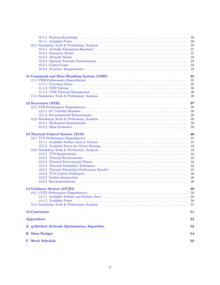
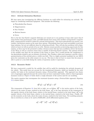
The EM-1 payload disposal trajectory places ARTEMIS on a trailing-edge lunar flyby with a periselene
altitude of 3100 km; if no maneuvers at all are performed after disposal, ARTEMIS will be flung towards
the Sun upon passing the Moon. This was verified by simulations conducted using AGI’s System Toolkit
(STK) 9.0 [6], as depicted in Figure 2.
Page 4](https://image.slidesharecdn.com/71722d65-e3b3-454a-aee6-5eab4a02991a-150717011219-lva1-app6891/85/Cube_Quest_Final_Report-10-320.jpg)
![NASA Cube Quest Summary Document April 15, 2015
Figure 2: Position of ARTEMIS (green) with respect to Earth (light blue) and Moon (white), three days
after EM-1 disposal, given no on-board propulsion.
Therefore, ARTEMIS must include some on-board propulsion to successfully compete in the Lunar Derby.
Low-thrust maneuvers to achieve LLO are difficult to simulate, in part due to the complex pattern of flybys
and thrust arcs necessary to insert ARTEMIS into LLO from EM-1. Extensive simulations conducted by
researchers at Goddard Space Flight Center, Purdue University, and Catholic University [7] have, however,
demonstrated the feasibility of low-thrust maneuvering to achieve LLO from the EM-1 payload disposal
trajectory. Their findings are summarized in Table 3.
Table 3: Comparison of of low thrust maneuvers from EM-1 disposal to LLO.
Maneuver Summary System
thrust (mN)
Maneuver
duration
(days)
Aposelene x
Periselene (km)
Inclination (deg)
Trailing-edge Lunar flyby to
trailing-edge Earth flyby
0.5 231 6800 x 100 20
Trailing-edge Lunar flyby to
Earth-Sun L1
2.0 250 9993 x 1545 144
Antivelocity burn to highly
eccentric Earth orbit
3.0 223 6513 x 139 156
Leading-edge Lunar flyby to
apogee at Lunar orbit
2.0 171 350 x 50 165
Leading-edge Lunar flyby to
perigee at Lunar orbit
3.0 214 5571 x 101 32
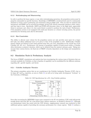
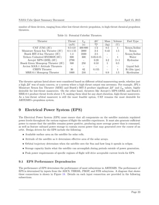
Assuming sufficient power input, the CubeSat Ambipolar Thruster (CAT) (detailed in Section 8.2.1) can
exceed the thrust level required in several of the simulations [8], implying the total maneuver time could be
decreased. While several of the simulated capture orbits violate Requirements ORB-02 and ORB-03, the
final orbit could be corrected by further maneuvers once ARTEMIS is within the Moon’s sphere of influence,
or by simulating with constraints placed on the final aposelene and periselene.
Page 5](https://image.slidesharecdn.com/71722d65-e3b3-454a-aee6-5eab4a02991a-150717011219-lva1-app6891/85/Cube_Quest_Final_Report-11-320.jpg)
![NASA Cube Quest Summary Document April 15, 2015
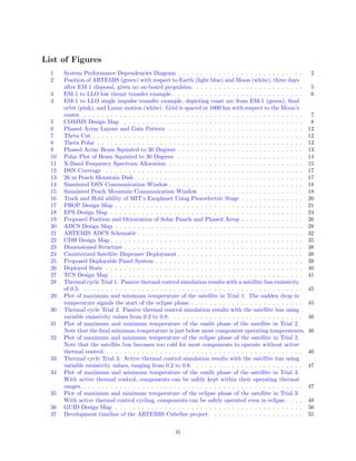
As a representative example of the simulation complexity, the first maneuver scenario [7] described in Table
3 is depicted in Figure 3 below. The larger image is in a Sun-Earth rotating coordinate frame, with the line
between the Sun and the Earth in yellow. Upon being released from EM-1, the simulated spacecraft would
immediately begin thrusting in an anti-velocity direction (red), increasing periselene altitude to reduce the
∆V imparted by the Lunar flyby. The spacecraft would then swing back towards Earth (contrasting Figure
2), and then shut off its thruster. Coasting along this ballistic trajectory lets the spacecraft flyby Earth,
with its apogee approaching the Sun-Earth L1 distance. At some point it begins to thrust in the velocity
direction (green), and subsequently alternates coast and thrust arcs until it is inserted into its final Lunar
orbit, 231 days after EM-1 disposal.
Figure 3: EM-1 to LLO low thrust transfer example.
Another option is a low-thrust CubeSat maneuver from geosynchronous Earth orbit (GEO) to a 100 km
altitude LLO; assuming a 4kg 3U CubeSat and JPL’s MIXI thruster, providing 1 mN thrust, 3000 s specific
impulse, and 3.5 km/s total ∆V [9], the maneuver time was 365 days with a ∆V requirement of approximately
2.3 km/s. Accordingly, if a GEO to LLO transfer is chosen, ARTEMIS would likely need to launch close to
a year before EM-1 to remain competitive with the winners of Ground Tournament 4.
Low-thrust maneuvers are not the only choice available to the mission, however. As discussed in Section
8, several high-thrust chemical thrusters are available on a CubeSat platform. The low-thrust simulations
cited above required complex initial guesses, algorithms, and software. Therefore, orbit simulations and
analysis focused on minimizing the ∆V necessary for GEO to LLO and EM-1 to LLO transfer using chemical
propulsion options.
Accurate simulation demands accurate representation of the spacecraft’s equations of motion. Lunar orbit
trajectories in particular are highly perturbed and cannot be accurately represented using the standard
two-body problem, as discovered during the run-up to the Apollo missions [10]. The Moon itself is highly
heterogenous, sporting several mass concentrations or “masscons”. Furthermore, due to the Moon’s relatively
Page 6](https://image.slidesharecdn.com/71722d65-e3b3-454a-aee6-5eab4a02991a-150717011219-lva1-app6891/85/Cube_Quest_Final_Report-12-320.jpg)
![NASA Cube Quest Summary Document April 15, 2015
low mass, the tug of the Earth and Sun represent significant perturbing forces on any spacecraft in Lunar
orbit. Therefore, the STK ’CisLunar’ gravity model was chosen to simulate the equations of motion when
the spacecraft was within the Moon’s sphere of influence (approx. 61,600 km from its center [11]). This
model accounts for these major perturbing forces, using a spherical harmonics model for both the Earth and
Moon, and a point-mass model for the Sun.
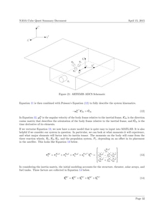
The optimization problem posed for a chemical propulsion maneuver from EM-1 to lunar insertion was to
minimize the ∆V expenditure of the system. A single impulsive maneuver was assumed. The resulting
aposelene and periselene altitudes were constrained to be between 300 km and 9,000 km to satisfy require-
ments ORB-02 and ORB-03, and the eccentricity of the new orbit with respect to the Moon was constrained
to be below 0.8 (elliptical). Secondary simulations demonstrated that Lunar orbits with eccentricity above
approximately 0.8 were quickly perturbed into parabolic or hyperbolic trajectories. The simulation was
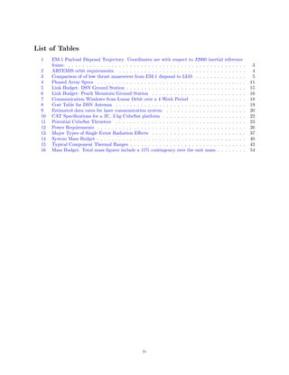
propagated for a month after EM-1 disposal, and the result is demonstrated in Figure 4.
Figure 4: EM-1 to LLO single impulse transfer example, depicting coast arc from EM-1 (green), final orbit
(pink), and Lunar motion (white). Grid is spaced at 1000 km with respect to the Moon’s center.
The optimizer arrived at an impulsive ∆V of 0.466 km/s in the antivelocity direction at the periselene of
the EM-1 coast arc to insert ARTEMIS into Lunar orbit, similar to a classic Hohmann transfer. Over the
simulated month, the mean aposelene was 9000 km, and the mean periselene was 1,272 km. Even accounting
for variations in the orbit (depicted as the band of overlapping pink ellipses) due to perturbations, the
orbit remains firmly within Lunar Derby requirements. Propagating the simulation for the duration of the
Page 7](https://image.slidesharecdn.com/71722d65-e3b3-454a-aee6-5eab4a02991a-150717011219-lva1-app6891/85/Cube_Quest_Final_Report-13-320.jpg)
![NASA Cube Quest Summary Document April 15, 2015
competition yields similar results. This impulsive ∆V far exceeds the capability of any existing small-sat
propulsion unit, suggesting chemical propulsion may not be feasible to achieve LLO from the EM-1 trajectory.
Reardon, et al [9] inspected high-thrust chemical propulsion maneuvers from GEO to LLO. Assuming a two-
impulse direct transfer, based on a Hohmann transfer, they found a 3U CubeSat (4 kg wet mass) required 1.8
km/s to achieve lunar orbit. A bielliptical transfer required close to double the ∆V of the quasi-Hohmann
transfer. As noted in Table 11, small-sat chemical propulsion units do not currently exist that can provide
that level of impulsive ∆V .
In conclusion, future simulation efforts and system design should focus on low-thrust electric propulsion ma-
neuvers from GEO or EM1 to LLO. While these maneuvers are time-consuming, choosing electric propulsion
increases the mass available to the communications subsystem, and with a sufficiently early launch to GEO,
ARTEMIS can remain competitive with EM1-launched competitors.
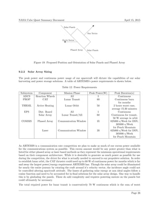
7 Communication System (COMMS)
The Communications System (COMMS) is the driving subsystem for the Cube Quest Challenge, and its
requirements are determined by the Challenge’s Operations and Rules document. It must be capable of
providing the greatest possible burst data rate over a 30-minute period as well as the greatest possible
aggregate data volume over a 28-day period. This data must be error-free to count for the competition. The
COMMS must also be capable of downlinking regular system telemetry down to ground stations. Lastly,
position determination may require some form of secondary communication system for tracking.
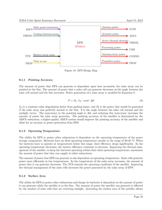
7.1 COMMS Performance Dependencies
The COMMS system, as the ultimate input to the cost function J(x), has mission priority over the other
subsystems, therefore resource allocation will be designed with the specific needs of COMMS in mind. The
performance of ARTEMIS’ communications system depends on multiple input parameters coming from the
other subsystems. These connections are shown below in Figure 5.
COMMS
ADCS
(Data)
EPS
J(x)
Pointing accuracy
Antenna/array power
Data transmission rate
STR
CDH
PROP
Antenna/array size
Data rate support
Comm windows
Figure 5: COMMS Design Map
7.1.1 Available Power
The amount of available power to the communication system is crucial to data transmission rates. The
quality of the received signal is determined by the link equation (1), which outputs the signal-to-noise ratio
Page 8](https://image.slidesharecdn.com/71722d65-e3b3-454a-aee6-5eab4a02991a-150717011219-lva1-app6891/85/Cube_Quest_Final_Report-14-320.jpg)
![NASA Cube Quest Summary Document April 15, 2015
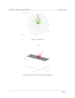
7.2.1 Phased Array Overview
A Phased Array consists of multiple antennas linked together to increase the overall aperture area. Phased
arrays offer many advantages. Each antenna transmits the same signal, but at a slightly offset phase from
its neighbor. This phase difference can be used to electronically steer the focus of the main lobe. This can
be done with normal RF antennas but the best results come from using multiple patch antennas arranged in
a close configuration on a flat surface. The size, number of patch antennas, and signal frequency determine
the gain of the phased array. For higher transmission rates; a high gain, high frequency system would
be the most desirable. ARTEMIS has limited physical resources available for a large, deployable, gimballed
antenna. A phased array is perfect for the flat, rectangular CubeSat form factor. Our proposed phased array
is constructed of 243 wafer-thin patch antennas measuring 1.435 x 1.176 cm each. They are constructed using
Teflon, a low dielectric material. The size of each patch was optimized to give the best efficiency at the given
carrier frequency [12]. The overall path efficiency is theoretically calculated to be 80.85%, much better than
the aperture efficiency of most parabolic dishes of the same size. This is marked advantage of phased arrays,
their individual elements can be tuned for optimum efficiency. The small patch antennas are arranged in a
rhombic pattern 6 and cover an area approximately 3U x 6U, the size of the satellite with deployable solar
panels. The greatest advantage in using a phased array is the fact that the beam can be electronically steered.
The directionality of the beam can be squinted ±30° without significant losses. This reduces pointing error,
minimizes ADCS requirements, and allows the solar panels to simultaneously face the Sun. Simulations were
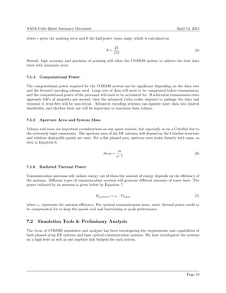
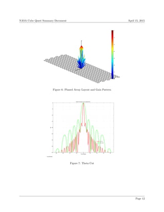
run [13] and gain plots for the phased array can be seen in Figures 6-10.
Table 4: Phased Array Specs
Parameter Value Units Comment
Antenna Size 60 x 30 cm 3U x 6U
Number of Elements 243 Rhombic Pattern
Dielectric Constant 2.03 Teflon (PTFE)
Overall Patch Eff. 80.85 % Excellent
Antenna Gain 30.46 dBi
Beam Width 3 deg. Slice phi=0
Max Squint Angle ±30 deg.
Page 11](https://image.slidesharecdn.com/71722d65-e3b3-454a-aee6-5eab4a02991a-150717011219-lva1-app6891/85/Cube_Quest_Final_Report-17-320.jpg)
![NASA Cube Quest Summary Document April 15, 2015
0
−5
−10
−15
−20
−25
−30
−35
15
30
45
60
75
90
105
120
135
150
165
−180
−165
−150
−135
−120
−105
−90
−75
−60
−45
−30
−15
−0
Phi = 0
Phi = 90
Theta TOT pattern cuts for specified Phi
Freq 8495 MHz
Figure 10: Polar Plot of Beam Squinted to 30 Degrees
Using a phased array has many engineering advantages. Flat panels are easier to construct than complex
gimballing mechanisms. If the dimensions of the CubeSat need to change, the phased array can morph
respectively and only the elements will need to be re-calibrated. The phased array also offers fault protection.
If one or multiple patches fail it will have little effect on the performance. Likewise, if the main element of
a parabolic dish or laser system fails the mission becomes a bust. Phased arrays have extensive heritage on
the ground and in space [14], because of this we think the technology is ideal if an RF system is to be used
on Artemis.
7.2.2 Phased Array Link Budget
A link budget has been formulated to determine the maximum data rate possible and the signal-to-noise
(SNR) link margin. When transmitting from lunar orbit, the main contributor to signal power degradation
is free-space path loss given by Equation 8.
Ls =
c
4πSf
2
(8)
From the equation we see that path loss decreases as the signal frequency increases. Ideally, ARTEMIS
would transmit in the 8-12 GHz X-band frequency spectrum. The Federal Communications Commission
(FCC) has allocated this frequency band for small sat communication. This band offers low atmospheric
attenuation, higher gain, and higher data rates. There are many commercial transmitters and receivers with
flight heritage designed to operate in the X-band spectrum. Higher frequencies such as Ka band (26.5-40
Ghz) exist, but they suffer from very high rain and atmospheric attenuation that could jeopardize the volume
transmission challenge over a continuous 30-day period. The efficiency of transmitters also decreases as the
signal frequency increases. An X-band solid-state power amplified (SSPA) only has an overall efficiency of
28% [15].
Page 14](https://image.slidesharecdn.com/71722d65-e3b3-454a-aee6-5eab4a02991a-150717011219-lva1-app6891/85/Cube_Quest_Final_Report-20-320.jpg)
![NASA Cube Quest Summary Document April 15, 2015
Figure 11: X-Band Frequency Spectrum Allocation
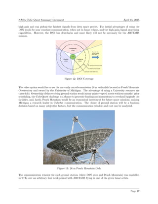
Two link budgets have been created for the phase array, one for each of the potential ground station receivers.
The largest, most advanced X-band capable ground station is NASA’s Deep Space Network (DSN) consisting
of three sites located around the world to provide constant deep space coverage. The receiving dish of interest
is the large 70 m diameter dish as it offers the highest gain and will be useful for comparison purposes. The
alternative ground station is the 26 m radio telescope owned by the University of Michigan located at Peach
Mountain Observatory near Dexter, MI. The Peach Mountain dish has not been operational for decades so
parameter values have been estimated for similar sized parabolic receivers.
Table 5: Link Budget: DSN Ground Station
Parameter Value Unit Comment
Receiver Diameter 70 m DSN Large Dish
Receiver Gain 74.18 dBi [16]
Transmitter Gain 30.46 dBi Calculated
System Noise Temp 21.3 dB-K Estimated
Transmitter Line Loss 0.5 dB From SMAD [17]
Receiver Line loss 0.5 dB Estimate
Required Eb
No
4.4 dB BPSK Plus R-1/2 Viterbi Decoding; From SMAD [18]
BER 10e−5 Bit Error Rate; From SMAD [18]
Transmitter Bus Power 40 W Orbital Average
Power Amplifier Efficiency 30 % From SMAD [18]
Losses 10 dB From SMAD [18]
Free Space Path Loss -222.3 dB At Average Earth Moon Distance
Data Rate 10 Mbps Maximum data rate transmitting to DSN
SNR 19.01 dB Calculated
Link Margin 14.61 dB Very Good
Page 15](https://image.slidesharecdn.com/71722d65-e3b3-454a-aee6-5eab4a02991a-150717011219-lva1-app6891/85/Cube_Quest_Final_Report-21-320.jpg)
![NASA Cube Quest Summary Document April 15, 2015
Table 6: Link Budget: Peach Mountain Ground Station
Parameter Value Unit Comment
Receiver Diameter 26 m Peach Mountain Radio Observatory
Receiver Gain 65.73 dBi Calculated
Aperture Efficiency 0.7 Estimated
Transmitter Gain 30.46 dBi Calculated
System Noise Temp 23 dB-K Estimated
Transmitter Line Loss 0.5 dB From SMAD [17]
Receiver Line loss 0.5 dB Estimate
Required Eb
No
1.89 dB Rate 2/3 QPSK Turbo coding; From SMAD [18]
BER 10e−10 Bit Error Rate; From SMAD [18]
Transmitter Bus Power 40 W Orbital Average
Power Amplifier Efficiency 30 % From SMAD [18]
Losses 10 dB From SMAD [18]
Free Space Path Loss -222.3 dB At Average Earth Moon Distance
Data Rate 30 Mbps Target
Spectral Efficiency 1.32
Required Bandwidth 23 Mhz Calculated
SNR 4.1 dB Calculated
Link Margin 2.21 dB
Link analysis of the two different ground stations provides interesting insight into potential communication
architecture. The large 70m dish has very high gain and a low system noise resulting in a very good SNR of
19.01. This gives a link margin of 14.61, which is sufficient highly to account for unexpected losses, pointing
errors, and component inefficiencies. The Peach Mountain Dish (PMD) is a respectably large dish with
sufficient gain for lunar missions. The receivers will not be as advanced as the DSN’s so more system noise
will be present in the signal. This can be mitigated by cooling the receivers, but is unlikely to be necessary.
One of the biggest factors determining downlink data rates is the required SNR and transmission encoding.
Readable bits can be sent at lower signal energies by using advanced forward encoding schemes. Common
encoding methods include BPSK, QPSK, and newer convulsion turbo codes. For example, using QPSK
with a 1/4 code rate the required SNR is only 0.75 dB [19]. However, this comes at the expense of reduced
spectral efficiency of only 0.49 bps/Hz. RF bandwidth is a limited and tightly controlled resource. Therefore,
efficient use of the allocated bandwidth is essential. For the Peach Mountain link budget, we chose a QPSK
rate 2/3 turbo code which makes efficient use of bandwidth at a low SNR. For a bandwidth of only 23 MHz,
ARTEMIS would be able to downlink at a rate of 30 Mbps and a SNR of 4.1 dB. This data rate is exceptional
for a CubeSat and would be fast enough to stream Hi-Def video from lunar orbit. While the link margin is
small, the mission parameters and environment can be tightly controlled to optimize data rates.
One of the biggest inefficiency factors in the link budget is the solid-state power amplifier. It draws 40 W
of bus power, but at 30% efficiency only provides 12 W of RF power to the antenna. Traveling Wave Tube
Amplifiers can exceed 60% efficiency but are bulky and too massive to be flown on a CubeSat. Ideally,
technology maturation will increase component efficiency and help push low-power data rates higher.
7.2.3 Ground Station and Communication Window
The Deep Space Network (DSN) is a world-wide network of advanced antennas and communication facilities.
There are a total of three sites located in California, Spain, and Australia. Each site is spaced approximately
120° apart to provide uninterrupted contact with deep space missions. The facilities offer exceptional tech-
nology in signal processing, radar telemetry and supporting space missions. The large 70 m dish has very
Page 16](https://image.slidesharecdn.com/71722d65-e3b3-454a-aee6-5eab4a02991a-150717011219-lva1-app6891/85/Cube_Quest_Final_Report-22-320.jpg)
![NASA Cube Quest Summary Document April 15, 2015
Table 7: Communication Windows from Lunar Orbit over a 4 Week Period
Mean Weekly Contacts Mean Duration [min] Total Contact Time [min]
DSN 58 223.7 12975
Peach Mountain 19 224.9 4272
Ratio (DSN/PM) 3.04
Figure 14: Simulated DSN Communication Window
Figure 15: Simulated Peach Mountain Communication Window
As seen from Table 7, the total contact time for the DSN is three times greater than for Peach mountain.
This makes sense as there are a total of three DSN ground sites vs. one Peach Mountain ground site.
However, this is does not mean that use of the DSN would allow for three times the data to be sent, as
Page 18](https://image.slidesharecdn.com/71722d65-e3b3-454a-aee6-5eab4a02991a-150717011219-lva1-app6891/85/Cube_Quest_Final_Report-24-320.jpg)
![NASA Cube Quest Summary Document April 15, 2015
NASA limits the downlink data rate from DSN targets to 10 Mbps [20] to avoid overloading the system
when multiple targets are tracked simultaneously. Normally, 10 Mbps is sufficient for deep space satellites
transmitting telemetry and scientific data. For a capable communication satellite such as ARTEMIS, with
a high-gain transmitting antenna, this is a limiting rate. As it so happens, the link budget using the Peach
Mountain site is sized using a 30 Mbps downlink rate, three times that of the DSN network. This means
that the even though Peach Mountain will not be in constant view of ARTEMIS, we would still be able to
downlink the equivalent volume of data over the 28-day challenge period, and potentially even more data
with improvements. The burst data challenge will be severely hampered by the DSN data limit. The Peach
Mountain site, with capable receivers able to handle the high data rates, would be much more successful at
the challenge. Therefore, it is our recommendation to use a privately owned site to accomplish the burst
challenge.
With total data volume being equal, cost becomes an important factor in determining which ground site
to use. The DSN charges for time based on a costing model that weights the number of contacts and dish
used. The estimate price was calculated using the excel document provided by JPL [16]. Peach Mountain
would be owned by the University of Michigan and access time will be considered free. Unfortunately, this
dish is nonfunctional and significant capital, estimated at $2.5 million, would be needed to bring it online.
However, as mentioned before, the money can be raised through research partners/grants and the dish would
become a vital resource to the University for future missions and scientific research. A cost table 8 can be
seen below.
Table 8: Cost Table for DSN Antenna
Antenna Service Hours per No. Tracks No. Weeks Pre-, Post- Total Total Cost
Size Year Track per Week Required Config. Time Reqd. for period
(meters) (year) (hours) (# tracks) (# weeks) (hours) (hours) Fiscal-Year
70 2018 0.5 1.0 1.0 0.50 1.0 3,134
34BWG 2018 3.75 58.0 4.0 10.00 880.0 4,618,910
From Table 8 we see that the cost to use the DSN for the four week data challenge is exorbitantly high, even
using the smaller 34 m dishes. Concluding the ground station review, we recommend to not use the DSN
as it offers no advantages and is prohibitively expensive. Instead, the University should use funds to restore
the Peach Mountain 26 m RF dish, as this would be the most beneficial use of resources.
7.2.4 Laser Communication
Laser communication could be called the “home run solution” to ARTEMIS’s communications subsystem:
high risk, high reward. In general, laser communications subsystems provide extremely high data rates, but
dramatically increase system complexity. Transmitting the laser to the ground station requires an extremely
precise and stable ADCS system. The TRL for laser communications is low, and even lower for the Cubesat
platform. ARTEMIS could serve as a TRL-raising mission for Cubesat laser communications, but this may
require external expertise, cooperation and funding.
Table 9 estimates the achievable data rates for a 0.5 W output laser communication system aboard ARTEMIS.
If the laser power output is boosted to 2 W, the data rates can be quadrupled.
Potential ground stations include NASA’s 1-m Optical Comm. Telescope Lab at Wrightwood, California;
White Sands, New Mexico; Tenerife, Spain; and, potentially, military or experimental sites. The University
of Michigan could build their own laser ground terminal, which would have the same communication window
as the Peach Mountain dish discussed in the phased array, Section 7.2.3.
Page 19](https://image.slidesharecdn.com/71722d65-e3b3-454a-aee6-5eab4a02991a-150717011219-lva1-app6891/85/Cube_Quest_Final_Report-25-320.jpg)
![NASA Cube Quest Summary Document April 15, 2015
Table 9: Estimated data rates for laser communication system.
Parameter Value Units
Assumptions
Range 400,000 km
Flight laser power 0.5 W
Diameter of flight telescope 5 cm
Diameter of ground telescope 100 cm
Link zenith angle 70 °
Flight terminal pointing allocation 15 µrad
Ground detector efficiency 75%
Link margin 3 dB
Slot width 200 ps
Data Rates
Daytime 165 Mb/s
Evening 185 Mb/s
Nighttime 200 Mb/s
To achieve data transmission through a laser, ARTEMIS would have to point the laser towards the ground
station with 120 arcsecond accuracy. The ground station requires a rough 1000-plus pixel CCD camera (17
mrad field of view) to acquire the beacon signal. After acquiring beacon lock, a fine pointing mirror on
ARTEMIS could keep the downlink beam centroid within 2-4 arcsec of the ground station camera centroid.
The Massachusetts Institute of Technology (MIT) Space Systems Laboratory’s Exoplanet Sat is being de-
signed to a 1 arcsec pointing capability using a two-axis piezoelectric translation stage as seen in Figure 16.
If successful, a similar design could be adopted for ARTEMIS. The ARTEMIS ADCS subsystem would also
be used to eliminate sensor noise and jitter by feeding forward estimated disturbances from the reaction
wheels to the optics [21] as seen in Figure 16.
Figure 16: Track and Hold ability of MIT’s Exoplanet Using Piezoelectric Stage
In summary, an accurately size onboard laser communications system is expected to consume approximately
3 kg of mass, 10 W of power, and 1.5U of volume. Besides the technical difficulties, laser is susceptible to
cloud cover and atmospheric distortion. At its current TRL, laser communication has only been flown for
NASA concept testing. The technology space for CubeSat level laser communication systems should continue
to be monitored until the launch date. The technology is developing rapidly and in three years it may end
up being the most desirable option. Michigan can help accelerate the pace of space laser communication
systems by developing ARTEMIS on parallel tracks: one RF and one laser version.
Page 20](https://image.slidesharecdn.com/71722d65-e3b3-454a-aee6-5eab4a02991a-150717011219-lva1-app6891/85/Cube_Quest_Final_Report-26-320.jpg)

![NASA Cube Quest Summary Document April 15, 2015
case power required for the CAT thruster and satellite bus systems. A solution involving panels under
ideal inclination angles for the duration of the trip using 28.3% efficient Spectrolab UTJs will generate 38.3
mW/cm2
at its maximum power point [22]. Each 3U face of the solar array will have seven 32 cm2
solar
cells and therefore generate 8.58 W. Including a standard pre-alpha mission phase margin of 30% means the
8.58 W per 3U panel would need to source 91 W of power. This ultimately requires a deployed solar array
that is slightly larger than 10U x 3U. This is once again a solar panel that is assumed to be perfectly facing
the Sun and operating exactly at its maximum power point.
In summary, the current 6U x 3U array would not be sufficient to power ARTEMIS’s trip to the Moon.
Advances in solar cell technology could make it a possibility, but they would need to be drastic. For instance
to use an 8U x 3U array, the solar cells would have to reach 38% efficiency, while a 6U x 3U array would
need 51% cell efficiency.
9.2.3 Power Storage
ARTEMIS is expected to experience regular eclipse intervals during lunar orbit and some of these eclipses
could be up to 4 hours in length. This dark environment will become quite cold and staying in it for
any duration longer than an hour without active heating would put some of our components beyond their
survivability limits. To prevent this, ARTEMIS will be actively heating its components during eclipse periods
using power stored when the spacecraft was in the Sun. The degree and method of heating chosen requires
a significant amount of power and represents the largest necessary amount of power storage for ARTEMIS.
The thermal subsystem is base-lining a solution that would draw 50 W for over two hours to maintain
component capabilities during a worst case eclipse scenario, as described in Table 12. This means the
storage capacity of ARTEMIS, accounting for the 30% margin, would need to be 130 Wh. However, as
this requirement is based entirely on thermal control, it could be reduced with advances in its capabilities
or by choosing less power intensive method. Additionally, having large amounts of storage capacity could
also be quite advantageous for the competition. ARTEMIS will also require high capacity storage for the
capture maneuver burns, thus afterwards there will be a depleted storage well on the satellite which would be
available for other systems after recharging. The relatively long sunlight times and short eclipse times should
allow us to rapidly charge the batteries, thus providing ample power even for high-demand subsystems. This
power would also allow us to broadcast even when the Sun is eclipsed during a transmission window, and
would provide an emergency reserve during lunar eclipse, when the Sun would be obstructed by the Earth
for an extended period of time.
We are base-lining the use of Lithium Ion batteries to supply the necessary 130 Wh of power to ARTEMIS. It
would require 1.2 kg of Li-Ion batteries to supply this amount of power. We are base-lining Li-Ion batteries
due to the fact that they have the same cycling ability as Nickel Hydrogen and Nickel Cadmium batteries
but can supply twice as much power. They also have a long flight heritage and can be bought at low cost,
which makes them more reliable and cost-effective than Lithium Polymer batteries that are currently being
researched.
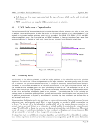
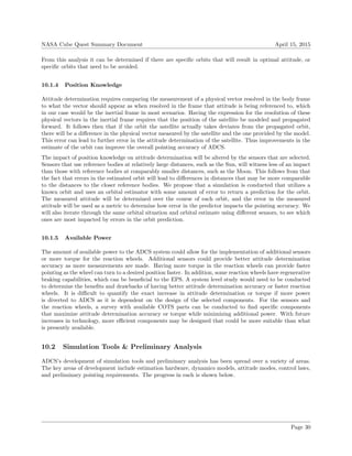
10 Attitude Determination and Control System (ADCS)
The Attitude Determination and Control System (ADCS) has two primary and related responsibilities. First,
the ADCS must estimate the satellite’s attitude using a variety of sensors and filters. Then, the ADCS must
be able to control the satellite’s attitude. This is necessary for the successful operation of components such
as the transmitter, solar panels, and propulsion system. Design drivers for the ADCS include the following:
• Orbital trajectory and selection of communication system will drive the required pointing accuracy.
Page 27](https://image.slidesharecdn.com/71722d65-e3b3-454a-aee6-5eab4a02991a-150717011219-lva1-app6891/85/Cube_Quest_Final_Report-33-320.jpg)
![NASA Cube Quest Summary Document April 15, 2015
algorithms should include simple algorithms such as the TRIAD algorithm and the q-Method [23], as well as
more computationally expensive methods such as the Kalman Filter, Extended Kalman Filter, Multiplica-
tive Extended Kalman Filter [24], and Complementary Filters [25]. ADCS may also incorporate a variety of
feedback methods, such as linearization about a given state or non-linear SO(3)-based control laws, as seen
in Zlotnik [26].
10.1.2 Sensor and Actuator Volume
The ability for ADCS to determine the attitude of the satellite and to achieve and maintain a desired
orientation or attitude rate is dependent on the selection of sensors and actuators which is limited by the
size constraints of the CubeSat. For attitude determination, a Star Tracker alone would be sufficient; however,
it becomes useless if it is blinded by light from the Moon, Sun, or the Earth. As this blinding is expected
to occur regularly, ARTEMIS will require additional attitude sensors for redundancy. Potential redundant
sensors include additional Star Trackers, horizon sensors, gyros, or sun sensors and photodiodes.
In order to determine the optimal number of attitude sensors, we can conduct a simulation with Orbits data
to maximize the ADCS sensor coverage time while minimizing the mass and volume. We can check how
frequently a Star Tracker tracks stellar targets and determine the relationship between adding additional
Star Trackers and increased stellar target tracking time. We can also simulate with different combinations
of attitude sensors and determine if utilizing other sensors with the Star Tracker provides enough time to
track attitude.
Attitude control is conducted by the ADCS actuators, which are traditionally reaction wheels. A reaction
wheel consists of a brushless motor attached to a flywheel which spins and produces a torque on the flywheel
that acts on the CubeSat with an equal magnitude but opposite direction. Having bigger reaction wheels
provides additional torque and faster control for the CubeSat at the cost of using more mass and volume.
The relationship between mass/volume with reaction wheel torque cannot be directly computed because
suppliers design their commercial off-the-shelf reaction wheels to have a similar mass or volume but different
torques and saturation speeds. A preliminary estimate can be made by conducting a survey with currently
available reaction wheels, categorized by different suppliers, to create a trend between mass/volume and
torque and saturation speeds. When the communication system is finalized and pointing accuracy require-
ments are determined, these estimates can be evaluated to find a supplier that designs reaction wheels that
fit our mass and volume constraints.
10.1.3 Orbital Parameters
The ability for ADCS to determine the attitude of the satellite depends on the orbital environment of
the satellite and the reference bodies that it will have available during the course of these orbits. Attitude
determination requires that the physical vectors from the satellite body to various objects, such as the Earth,
Sun, Moon, or other distant body, be measurable by on-board sensors. Thus, if the the line of sight required
for a measurement is blocked, it will disable that measurement from being utilized in attitude determination.
Blockages in line of sight are highly dependent on the orbit that the satellite is in. Orbits with periods of
eclipse will result in the loss of both coarse and fine sun sensors as an attitude measurement device, while
they may result in higher star tracker accuracy due to less saturation. Similarly, lunar horizon sensors may
be impacted by the shape of the orbit around the Moon. These trades are related highly to the particular
accuracy of a sensor as well as the number of environment it can be utilized in.
We propose that orbital simulations are conducted that put the satellite through a variety of orbital envi-
ronments (preferably with lunar-Earth, lunar-Sun, and Earth-Sun eclipses) so that we can determine how
each orbit impacts the utility of each different sensor. By taking the line of sight data provided by these
simulations, we can input this data into our attitude algorithms and analyze the accuracy of our estimator.
Page 29](https://image.slidesharecdn.com/71722d65-e3b3-454a-aee6-5eab4a02991a-150717011219-lva1-app6891/85/Cube_Quest_Final_Report-35-320.jpg)
![NASA Cube Quest Summary Document April 15, 2015
For instance, if the normal vector for a solar array appears as 0 0 1
T
in the body frame, we may declare
that the vector to the Sun appears as 0 0 1
T
when resolved in the body frame for the best angle of
incidence. From this we can now compose a set of vectors that we’d like to satisfy (such as solar arrays
towards the Sun, communications systems towards the ground, or ADCS sensors towards their operational
references). Then we may apply a solution method such as the q-Method or QUEST algorithm, which can
be found in de Ruiter, et al [23]. A MATLAB script that finds the optimal attitude using the q-Method can
be found in Appendix A.
10.2.5 Control Laws
Our primary investigative focus thus far has been the application of control by utilizing the direction cosine
matrix directly, following the work of Forbes, et al [26, 27]. A proportional-derivative control law that
provides this is given below.
τBC
b = kpPa(E)v
− kdωbd
b (15)
In this equation, τBC
b is the applied torque resolved in the body frame, kp is the proportional gain, Pa(·)
is the skew-symmetric projection operator such that Pa(U) = 1
2 (U − UT
), E is the rotation error matrix
defined by E = Cbd = CbiCT
di, where Cdi describes the desired attitude, (·)v
is the vectorizing operator such
that (u×
)v
= u, kd is the derivative gain, and ωbd
b is the angular velocity of the body frame, relative to the
desired frame, expressed in the body frame. We’d like to explore the potential for using this control law as
it would allow us to bypass parameterizing the direction cosine matrix.
To utilize this equation above, we will need to find an expression for ωbd
b , the angular velocity of the body
frame, relative to the desired frame, expressed in the body frame. This can be found using the following
equation.
ωbd
b = ωbi
b − ωdi
b (16)
The expression for the first term on the RHS can be produced by gyro measurements on the satellite. The
expression for the second term on the RHS is not easy to find analytically, but may be obtained by taking
the desired attitude at two times separated by a small time step, ∆t. Using the definition of the derivative
and Poisson’s equation, we can produce the following equation, which will give us a more usable expression.
ωdi
d = Pa
Cdi(t + ∆t)CT
di(t) − 1
∆t
v
(17)
It does assume that ∆t is small enough that the angular velocity physical vector is constant over ∆t.
Simulations can show how big ∆t can grow before significant error appears.
10.2.6 Accuracy Requirements
The ADCS accuracy requirement is derived by the antenna pointing requirement as determined by COMMS
in Section 7.1.3. If the laser communication system is selected, it is desired to have an extremely precise
pointing accuracy. In comparison, a phased array system could provide more flexibility in optimal attitude
and required accuracy requirements. A preliminary pointing accuracy for a laser communication system is
on the order of 3−9 mrad [28]. This is considered conservative, as lunar and deep-space spacecraft typically
point RF antennas with precisions to within 3 mrad. Current COTS components can currently provide a
pointing accuracy of ±0.01°, or 0.17 mrad [29].
Page 34](https://image.slidesharecdn.com/71722d65-e3b3-454a-aee6-5eab4a02991a-150717011219-lva1-app6891/85/Cube_Quest_Final_Report-40-320.jpg)
![NASA Cube Quest Summary Document April 15, 2015
11 Command and Data Handling System (CDH)
The Command and Data Handling System (CDH) must handle all on-board computing and data management
tasks [30]. These tasks will include monitoring the health of the satellite, preparing data for transmission
to Earth, ADCS algorithms, and any autonomous operations while in orbit. The CDH must handle all of
these reliably while exposed to solar radiation whenever ARTEMIS is not in eclipse. As a result, the effects
of radiation on the flight computer will be a primary consideration. Specific design drivers for the CDH
include:
• Redundancy or protection in case of event upsets due to solar radiation.
• Other satellite subsystems will determine the processing speed and memory requirements.
11.1 CDH Performance Dependencies
The performance of our Command and Data Handling system determines the capabilities of several other
subsystems. The performance of the CDH is related to the power, volume, and thermal control provided
to the system. Abstractly, the CDH outputs processing speed, or the number of computations per second
that other subsystems can utilize. These inputs and outputs are shown below in Figure 22. The inputs to
CDH are discussed in detail in the sections following the figure. The main subsystems which depend on
the processing speed of the CDH are COMMS and ADCS. The CDH must also be able to withstand the
radiation environment in space for the duration of its mission. While not modeled directly as an input,
radiation will be a significant consideration in any models or design decisions.
CDH
STR
(Processing)
EPS
COMMS
ADCS
Redundant computers
Processing power
Data rate support
Algorithm speed
THRML
Cooling of processor
Figure 22: CDH Design Map
11.1.1 Processor Power
The processing speed of the flight computer is related to the amount of power it is provided. In general,
higher power allows for a higher speed computer. However, a specific trend for this relationship is not
known. A second consideration is the performance of the same flight computer when given different amounts
of power.
To determine the first relationship, we advise that as the full satellite design date approaches, power and
processing speed data be gathered for a number of COTS CDHs and flight computers. This will allow for an
approximate trend to be developed for the most advanced technology available. Determining the relationship
between input power and processing speed for a given flight computer will require more experimentation.
Page 35](https://image.slidesharecdn.com/71722d65-e3b3-454a-aee6-5eab4a02991a-150717011219-lva1-app6891/85/Cube_Quest_Final_Report-41-320.jpg)
![NASA Cube Quest Summary Document April 15, 2015
Table 13: Major Types of Single Event Radiation Effects
Event Type Event Description
Single Event Upset Single bit-flip, information can be lost, temporary
Single Event Latch Up Inadvertent creation of a low resistance path within
MOSFET, requires reset of circuit/computer
Single Event Burn Out [31] High current burns out transistor,
can damage unprotected circuits
Single Event Gate Rupture [32] Large electric field permanently damages MOSFET
The first two types of events are detrimental to a spacecraft’s mission but typically do not cause permanent
damage. The second two types of events, however, can permanently damage a circuit or flight computer to
beyond an operational level. If redundant systems are not present, this can cause a complete mission failure.
There are two primary ways to guard against system failure due to solar radiation. The first way is to
physically shield the flight computer and other sensitive electronics with a barrier. This serves to block some
of the radiation from reaching the electronics. The second method is to build redundancy and error checking
into the hardware, software, or both. One example of a hardware redundancy is to fly two separate flight
computers, with one serving as a backup in case the primary CPU is damaged.
There are several common types of software redundancies, including watchdog timers and storing copies of
the main program code in several independent locations. Watchdog timers look for a periodic OK signal
from the flight computer and reset the computer if it is not received [33]. If multiple copies of the code
are flown, they system can read and vote on the best copy to run. In addition, the system can repeat this
process at set time intervals to ensure proper voting. We must also consider the total radiation dose we
expect over the duration of the mission and ensure that this does not cause a system failure.
In addition to protecting the system from radiation, CDH must also consider the transfer of data around
the satellite and to the ground. Specifically, we must determine how much data will be generated by each
subsystem and how fast it must be transmitted. For example, data from attitude sensors must be transmitted
quickly to perform attitude estimation. We must also determine how much telemetry we will take and how
long we will store that information. Finally, we must consider how we will transfer data and send commands.
Several standard communication protocols exist for this purpose, including I2C, SPI, and UART.
12 Structures (STR)
ARTEMIS will have a custom 6U structure that houses all of the avionics, propulsion, and thermal control
subsystems. The structure will be designed to satisfy all of the individual subsystem mechanical requirements.
In addition, the structure will be designed to the following SLS secondary payload and Cube Quest mechanical
requirements:
• Overall dimensions of 100 mm x 227 mm x 340.5 mm (See Figure 23).
• Total System Mass no greater than 14 kg (See Table 14 or Appendix B for more details).
• Ultimate factors of safety (FOS) of at least 1.4.
• Integrate with the NASA-provided 6U deployer.
• Survive the launch loads prescribed by the launch vehicle provider.
Page 37](https://image.slidesharecdn.com/71722d65-e3b3-454a-aee6-5eab4a02991a-150717011219-lva1-app6891/85/Cube_Quest_Final_Report-43-320.jpg)
![NASA Cube Quest Summary Document April 15, 2015
Figure 23: Dimensioned Structure
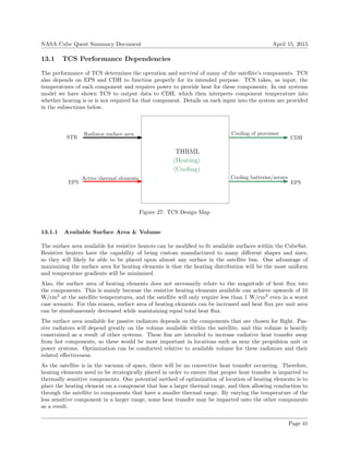
12.1 STR Performance Dependencies
The ARTEMIS structure will be designed mainly to the 6U deployer mechanical constraints and the expected
launch environment loads. By satisfying these constraints, ARTEMIS will safely integrate to the launch
vehicle and survive the launch into orbit.
12.1.1 6U CubeSat Deployer
According to the Cube Quest Operations and Rules document, NASA will provide, at no cost, a Planetary
Systems Corporation model 6U Canisterized Satellite Dispenser (CSD) [34] to those CubeSats selected for
EM-1. A rendering of ARTEMIS’s deployment from the 6U CSD can be seen in Figure 24. All mechanical
and electrical interfaces will be designed to comply with the 6U CSD requirements. According to the CSD
Payload Specification document [35], “the two tabs and the structure that contacts the CSD ejection plate
on the -Z face are the only required features of the payload. The rest of the payload may be any shape that
fits within the max dynamic envelope.” The mechanical design of ARTEMIS will be completely custom to
accommodate the 6U CSD requirements and other subsystem mechanical requirements.
Figure 24: Canisterized Satellite Dispenser Deployment
Page 38](https://image.slidesharecdn.com/71722d65-e3b3-454a-aee6-5eab4a02991a-150717011219-lva1-app6891/85/Cube_Quest_Final_Report-44-320.jpg)
![NASA Cube Quest Summary Document April 15, 2015
12.1.2 Environmental Requirements
The Space Launch System (SLS) Secondary Payload User’s Guide (SPUG) currently does not describe the
predicted launch loads or required environmental testing for the EM-1 CubeSats [36]. However, the 6U CSD
is qualified for a 3,750 N reaction load capability [37]. For a 14 kg CubeSat, that will correlate to a maximum
total RSS payload response of 26 g’s. Since the environmental loads are not provided yet, ARTEMIS will
be currently designed to withstand 26 g’s of maximum acceleration throughout Random Vibration, Shock,
Acceleration, and Sine Burst testing. These levels correlate to 18.6 g’s before taking in to account the FOS
of 1.4.
ARTEMIS will be built with space-rated, low-outgassing materials. All components will have a Total Mass
Loss (TML) of under 1.0%, and a Collected Volatile Condensable Materials (CVCM) of under 0.1%. A
thermal vacuum chamber will be used to bakeout the flight CubeSat to allow the materials to outgas before
delivery and launch.
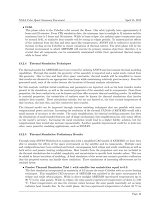
12.2 Simulation Tools & Preliminary Analysis
The specific mechanical requirements for ARTEMIS are developed to accommodate each subsystem. Due to
the current state of most subsystems, only general requirements are set for the structure. As the fidelity of
each subsystem matures, specific structural requirements will be added to accommodate each subsystem.
12.2.1 Mechanical Requirements
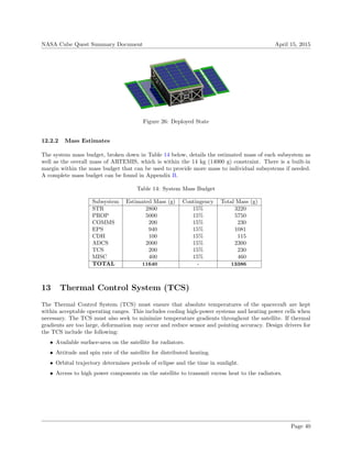
The main mechanical requirements for ARTEMIS are the usable surface area, volume, and mass throughout
the spacecraft. External and internal surface area is required for communication antennas, solar panels,
attitude sensors, thruster nozzles, and radiators. The allowable volume inside the spacecraft will be used
to efficiently pack fuel, batteries, actuators, and processing units, among the other required hardware. The
mass of each subsystem and its components will be carefully maintained to provide additional mass to certain
subsystems if needed.
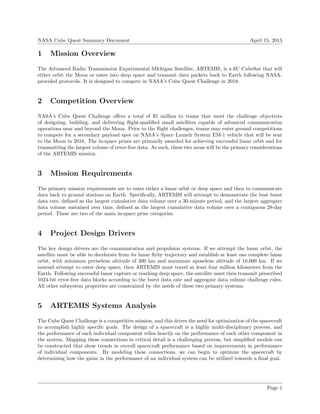
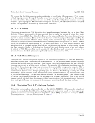
ARTEMIS will require a deployable panel system for an optimal solar cell surface area and phase array
antenna design. Figure 25 shows a proposed deployable panel system from its stowed configuration to the
fully deployed state. Figure 26 is another view of the proposed deployable panel system, with 49 solar cells
which all face in the same direction. A gimbaling system for the deployable panels may be needed to control
the panels for more optimal power generation and communication operations.
Figure 25: Proposed Deployable Panel System
Page 39](https://image.slidesharecdn.com/71722d65-e3b3-454a-aee6-5eab4a02991a-150717011219-lva1-app6891/85/Cube_Quest_Final_Report-45-320.jpg)
![NASA Cube Quest Summary Document April 15, 2015
The number of heating elements can be reduced by placing components that need to be in a certain tem-
perature range near each other so heat can be transferred via conduction and less power will be required to
heat. It is important to place the components with similar thermal ranges as close as possible to each other
in order to increase the power efficiency of the active thermal control.
The thermometers will be key in proper active thermal control, because they are the inputs into the command
of the heating elements. For this reason, the thermometer location relative to the heating element and
component are important to consider to ensure proper heating. Multiple thermometers per component
would be desirable to obtain the range of temperatures within the component. By knowing the range of
temperatures with certainty from the thermometers, active thermal control will become more effective at its
goal.
13.1.2 Available Power for Active Heating
The power available for the TCS is directly related to the amount of heat flux that is available to be
transferred to the thermally sensitive components. By increasing the amount of power available for the
TCS, the components will be able to be heated properly in a shorter amount of time. Also, for some values
of power, surface emissivities will become less important because the active thermal control will become
more and more capable of properly controlling component temperatures.
There are obvious drawbacks to pursuing maximum power consumption for the TCS, especially because other
satellite subsystems such as propulsion and communication will inherently require high power capabilities.
For this reason, an optimal condition for the power available for active thermal control will likely not be the
maximum available power. The location and surface area available for active thermal control is much more
probable in influencing the final design of the TCS due to power constraints.
13.2 Simulation Tools & Preliminary Analysis
The TCS subsystem has determined requirements for operation, and analysis has been performed to de-
termine how to fulfill these requirements. ANSYS has been used as a main resource for running thermal
simulations, and this method has been further explained in the subsequent subsections. From these results,
we have been able to make recommendations and conclusions on potential methods of successful thermal
control.
13.2.1 TCS Requirements
The main purpose of the TCS is to ensure the components are kept within their operating temperatures.
Our first requirement is to ensure that the temperature gradient requirements for the satellite are met. If
thermal gradients are too large on the structure, deformation may occur and cause the accuracy of sensing
components to be decreased; therefore, thermal gradients shall be kept to a maximum of approximately 100
°C within the satellite. Another requirement of the TCS is to ensure that all thermally sensitive components
remain within their survivable (and often operational) temperature ranges. This is crucial to ensure that
components do not become damaged by exceeding their specified temperature ranges [38]. In space, due to
extremely low residual pressure, only conductive and radiative heat transfer modes are significant; thus the
TCS system design must focus on using these means to control the thermal gradients.
Page 42](https://image.slidesharecdn.com/71722d65-e3b3-454a-aee6-5eab4a02991a-150717011219-lva1-app6891/85/Cube_Quest_Final_Report-48-320.jpg)
![NASA Cube Quest Summary Document April 15, 2015
Table 15: Typical Component Thermal Ranges
Component Operation Temp. (°C) Survival Temp. (°C)
Batteries 0 to 15 -10 to 25
Reaction Wheels -10 to 40 -20 to 50
Gyro/IMU 0 to 40 -10 to 50
Star Trackers 0 to 30 -10 to 40
CDH Box -20 to 60 -40 to 75
Power Box -10 to 50 -20 to 60
Solar Panels -40 to 80 -200 to 130
13.2.2 Thermal Environments
The space environment will determine the parameters that the thermal simulations and calculations must
take into account for the mission. The satellite will pass through periods of sun exposure and eclipse while
orbiting the Moon. The Earth’s magnetosphere does not extend to LLO, so ARTEMIS would be exposed
to deep space conditions during its entire lunar orbit phase. In this orbit, the approximate solar radiation
pressure experienced from the Sun at the Earth-Moon system is 1367 W/m2
. This radiation pressure
magnitude will influence the amount of thermal heat flux imparted onto the satellite from the Sun. It should
also be noted that the Moon is approximately 384,000 km (0.002 AU) away from the Earth; this means that
the minimum and maximum distance that the satellite could be from the Sun would be approximately 1 ±
0.002 AU. Because of this 0.2% difference in distance, the solar radiation pressure present at the Earth is
an acceptable approximation of the solar pressure that the satellite would experience in lunar orbit as well.
The effects of thermal radiation in the form of sunlight reflected from the Moon’s surface has an IR orbit
average of 430 W/m2
and a geometric albedo of 7% [39].
13.2.3 Thermal Enivronment Phases
There are three distinct thermal phases that need to be considered for the spacecraft’s thermal environment.
These phases are standing by on the launchpad prior to launch, transit to the Moon, and orbit around the
Moon.
• Launchpad
The CubeSat will be on the pad and placed into the SLS payload a few days before launch. Launch
will likely be from a moderately warm location, such as Florida’s Kennedy Space Center. The possible
effects of the temperatures and humidity should be taken into account to reduce the risk of damage
while waiting for launch on the pad. Simulations will be required to gain a better understanding of
the effects of the environment while on the launch pad. Based on the Space Shuttle Weather Launch
Commit Criteria and the KSC End of Mission Weather Landing document available on the NASA.gov
website, it can be assumed that the CubeSat could potentially experience temperatures in the range
of -18 to 38 °C during the launch phase [40].
• Transit to the Moon
This phase is defined as the trip from the Earth to the Moon, during which the CubeSat will be
exposed to constant sunlight for a duration of about 2 days. It is likely that the CubeSat will en-
counter Sun-side temperatures potentially exceeding 90 °C. Therefore, proper thermal insulation must
be incorporated to prevent overheating the systems onboard. A maximum of approximately 80 °C was
observed during simulation of the satellite in direct sunlight for 2 hours with an optimal emissivity
properties configuration. These simulation parameters will be explained in the analysis section.
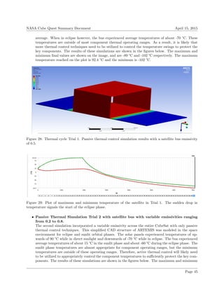
Page 43](https://image.slidesharecdn.com/71722d65-e3b3-454a-aee6-5eab4a02991a-150717011219-lva1-app6891/85/Cube_Quest_Final_Report-49-320.jpg)
![NASA Cube Quest Summary Document April 15, 2015
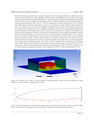
Figure 35: Plot of maximum and minimum temperature of the eclipse phase of the satellite in Trial 3. With
active thermal control cycling, components can be safely operated even in eclipse.
13.2.6 TCS Control Techniques
The TCS will utilize a combination of active and passive thermal control to ensure that all aspects of the
satellite remain within acceptable thermal ranges both while sitting on the pad prior to launch as well as at
all times during operation.
• Active Control
Active heating requires detection and control of component temperatures via the CDH system. The
CDH system will allow the temperatures of components to be interpreted, and then can send a signal
for heating to be activated or ceased depending on the desired versus current component temperature.
Active heating allows for higher resolution control of temperatures of specific components in the Cube-
Sat relative to passive control. Resistive heating, or patch heaters, can be used around more thermally
sensitive components within the satellite. This can be specifically applied to the batteries, as thermal
control is crucial to ensure their proper function.
• Passive Control
The satellite can utilize a passive thermal control system for the sake of simplicity and size constraints.
Passive TCS will also decrease the chance of failure of the TCS as a result of its simplicity. A low spin
rate could also be utilized to more evenly distribute the thermal load on the satellite. One potential
component is Multilayer Insulation (MLI), due to its success in past space missions. MLI is used to
prevent both excessive heat loss from a component as well as excessive heating from environmental
fluxes. Another potential solution is conductive thermal ducting within the satellite. Highly conductive
materials, connected from hot components to cooler components, could be utilized to distribute heat.
These materials could be either metals, such as copper, or composites, such as graphite fibers [41].
Space rated paint can be used to enhance both heat absorption and radiation. White paint could be
applied to the back sides of the solar panels of the CubeSat to ensure that heat generated by the panels
is radiated away from the satellite. Conversely, black paint could be applied to internal faces of the
CubeSat to ensure that, during cold periods, the internal heat is more efficiently preserved.
13.2.7 Surface Emissivities
The emissivity of the surfaces on the CubeSat will play an important role in thermal management due to
its impact on the retention and radiation of heat. The goal in selecting a surface emissivity is to maintain
as uniform and constant of a temperature in the satellite as possible. Simulations can be run with different
emissivities to optimize the distribution of surface emissivity values. One such example is that it may be
beneficial to have a high emissivity on the backs of the solar panels so the heat generated by the panels does
not overheat components.
Page 48](https://image.slidesharecdn.com/71722d65-e3b3-454a-aee6-5eab4a02991a-150717011219-lva1-app6891/85/Cube_Quest_Final_Report-54-320.jpg)
![NASA Cube Quest Summary Document April 15, 2015
Another option with these simulations is that they could allow for the investigation of variable emissivity
surfaces, to determine whether this might further optimize heat management. Variable emissivities for space
applications have been researched in the past by NASA [42], and Paragon is developing this technology [43]
for space radiator use. For this reason, variable emissivities may be a feasible technology for use due to their
current research progress as well as low power consumption values for a satellite system.
13.2.8 Recommendations
To keep vital components, such as batteries, reaction wheels, gyros, and star trackers, within their respective
operating temperatures, it is recommended that ARTEMIS employ a combination of passive and active
thermal control methods. A lunar mission will expose the CubeSat to near hot and cold soak conditions
which previous CubeSats have not had to consider. The system will include temperature sensors, peltier
coolers, resistive heaters, MLI, and an algorithm used to operate the active components once the sensors
breach a specified acceptable temperature threshold for the components.
• One thermoelectric heater can be used and strategically placed on the battery. This will allow the
battery to be heated or cooled as needed, particularly necessary when ARTEMIS is in an unusual
environment such as eclipse or waiting on the launch pad.
• Our simulation has shown that four resistive heating devices can be placed on the outside of other
components such as reaction wheels, gyros, and star trackers. As shown in our models, resistive
heaters will keep these core components within their operational temperature ranges. The main driver
for this device is to heat while in a worst case eclipse scenario. In this case, the heaters would operate
50% of the time at 50 W to keep the core components within operational ranges.
• Certain aspects of the structure and outer surfaces (bus panels) are covered with a paint-like variable
emissivity coating. This coating, as described above, can have its emissivity altered by passing a
current through it. The CDH could handle coating emissivity adjustments as ARTEMIS transitions
between sunlight and eclipse; this would allow the structure to hold or release heat depending on the
current state.
• A passive system will also be employed and it will consist of MLI strategically placed to decrease
radiative heat transfer throughout the satellite bus.
This is a feasible configuration for our mission based on the thermal models. From thermal modeling, we
can expect to see conditions that will require both an active heating system as well as passive. With our
prescribed thermal configuration, all components are expected to function continuously and normally.
14 Guidance System (GUID)
The Guidance System (GUID) has one primary responsibility. It must be capable of allowing the satellite’s
position and velocity to be determined to a high precision so that an accurate estimate of the orbital model
can be determined. Due to the nature of the Moon’s uneven mass distribution, any lunar orbit is subject to
significant perturbations, so the GUID system may need to be utilized frequently to provide an update for
the orbit estimate. Design drivers for the GUID system include the following:
• Eclipse periods with the Moon and Earth may disable use of the GUID system, making the accuracy
of the model determined outside of eclipse periods more important.
• Volume and surface must be dedicated to an RF system if it is required to determine the orbit.
• We are outside of the orbit of GPS satellites, making that an infeasible solution to determine our
position and velocity.
Page 49](https://image.slidesharecdn.com/71722d65-e3b3-454a-aee6-5eab4a02991a-150717011219-lva1-app6891/85/Cube_Quest_Final_Report-55-320.jpg)
![NASA Cube Quest Summary Document April 15, 2015
14.1 GUID Performance Dependencies
The GUID system is critical to the function of systems such as ADCS and PROP, as well as the optimization of
EPS and COMMS. In our model we have abstracted the GUID system to output position knowledge. ADCS
relies on knowledge of the orbital position to determine the reference physical vectors in the inertial frame,
and PROP uses both position and velocity to determine the required direction, duration, and magnitude of
thrusts. With better knowledge of position, EPS could improve power production and COMMS could yield
higher gain. A diagram that shows these connections is shown in Figure 36.
GUID
STR
(Position)
EPS
PROP
ADCS
Antenna size
Antenna power
Burn requirements
Pointing requirements
Figure 36: GUID Design Map
14.1.1 Available Volume and Surface Area
The GUID system will require the dedication of both volume and surface area for the hardware required. If
an RF system is used, it will require that a transmitter be housed in the system, as well as an omnidirectional
antenna that will take up surface area. Because this antenna will need to be omnidirectional, it follows that
it actually will not have a large physical aperture, as gain and omni-directionality are inversely proportional.
We propose that a simulation be conducted that could be used to determine the trend between the orbital
estimation accuracy and the transmitter size and effective antenna area, using the method described in
Cutler [44]. This simulation will take a known orbit with some given initial conditions and propagate it
forward. A set of RF patterns will be determined along the orbit using a variety of different transmitter
sizes and antenna areas, as well as introducing possible noise and error. We will then compare the orbit that
is predicted from each RF path to that of the actual one. We can see at which transmitter sizes and surface
areas do we began to escape the impact of the error in our system and reach acceptable levels of accuracy.
14.1.2 Available Power
The GUID system will need some amount of power to drive the RF systems required for the above method
[44]. As the power increases the impact of noise will decay and thus the error in the RF pattern will be
smaller. This will tend to increase the accuracy of the orbital determination method and, thus, improve the
performance of the GUID system.
We propose that a simulation be conducted to determine the relationship between the orbital estimation
accuracy and the power utilized by the GUID system. This simulation will take a known orbit with some
given initial conditions and propagate it forward. A set of RF patterns will be determined along the orbit
Page 50](https://image.slidesharecdn.com/71722d65-e3b3-454a-aee6-5eab4a02991a-150717011219-lva1-app6891/85/Cube_Quest_Final_Report-56-320.jpg)
![NASA Cube Quest Summary Document April 15, 2015
using a set of power levels, as well as models for system noise. We can then compare the orbit predicted using
our method to the actual one, and we can see at what power levels the impact of noise becomes negligible.
14.2 Simulation Tools & Preliminary Analysis
The initial work for the GUID system has been focused on studying the method for orbital determination,
also described in Cutler [44]. We have determined that as long as we can estimate our initial position and
velocity to some known tolerance, we can estimate the set of possible orbits that the satellite can be in. From
this we can determine what the RF behavior for those orbits should appear as, once we know something
about the communication system. This method of orbital determination has driven the direction of our
performance mapping for the GUID system to investigate using an RF system.
15 Conclusion
In conclusion, the Cube Quest Challenge is a complex mission that requires pushing the boundaries of Cube-
Sat technology. Our investigation has focused primarily on two areas: determination of mission feasibility
and development of models that can be used in optimization of a design. This approach allows us to provide
a baseline based on current technology as well as an idea on where the best development in technology lies
for the mission. We hope that we have provided a useful analysis of the mission and its features that may
be used in the development of a spaceflight vehicle that succeeds in the Cube Quest Challenge.
Page 51](https://image.slidesharecdn.com/71722d65-e3b3-454a-aee6-5eab4a02991a-150717011219-lva1-app6891/85/Cube_Quest_Final_Report-57-320.jpg)
![NASA Cube Quest Summary Document April 15, 2015
Appendices
A q-Method Attitude Optimization Algorithm
1 function [q opt,C bi opt] = q Method Optimize(s b,s i,w)
2 %q Method Optimization: This function is designed to find the optimal
3 %attitude of a satellite utilizing Paul Davenport's q-Method soltuion to
4 %Wahba's problem. It differs from the typical Wahba problem in that instead
5 %of utilizing measurements of physical vectors in the body frame, it uses
6 %what the measurement would optimally be in that flight mode. For example,
7 %in an optimzation problem where a satellite has a solar array with a
8 %normal vector given by [0 0 1]' in the body frame and we'd like to point
9 %the array at the Sun, we's use [0 0 1]' as one of our "measurement"
10 %vectors.
11
12 %The inputs of the function are s b (m by 3), s a (m by 3), and w (m by 1),
13 %where m is the number of physical vector that we are trying to optimize in
14 %our rotation. s b contains the desired normalized expression for the
15 %physical vectors in the body frame in a row fashion [x1 b y1 b z1 b], s i
16 %contains the normalized expression of the physical vectors in the inertial
17 %frame in a row fashion [x1 i, y1 i, z1 i], and w contains weightings for
18 %each of the physical vectors that determines their importance in the
19 %optimization.
20
21 %The objective function we are attempting to maximize is as follows:
22 %J(C bi) = Sigmaˆm {k=1} w k*s bk'*C bi*s ik
23
24 %The solving of this problem truly depends on finding the K matrix. To do
25 %this we must find the B matrix, which comes from taking the trace of our
26 %objective function and maniuplating it accordingly.
27
28 %Find the number of vectors we are actually optimizing.
29 m = size(w,1);
30
31 %Setup the transpose of the B matrix for looping.
32 B trans = zeros(3,3);
33
34 %Finding the the tranpose of the B matrix given our expressions of the
35 %physical vectors in the two frames.
36 for i = 1:m
37 B trans = w(i)*s i(i,1:3)'*s b(i,1:3)+B trans;
38 end
39
40 %Declaring B for ease of use later.
41 B = B trans';
42
43 %Declaration of three matrices in the K matrix.
44 k22 = trace(B trans); % 1 by 1
45 K 11 = B+B'-k22*eye(3); % 3 by 3
46 k 12 = [B(2,3)-B(3,2) B(3,1)-B(1,3) B(1,2)-B(2,1)]'; % 3 by 1
47
48 %Assembling the K matrix.
49 K = [K 11 k 12; k 12' k22]; % 4 by 4
50
51 %Take the eigenvalues of K, and select the largest eigenvalue and the
52 %corresponding eigenvector, which is the optimal quaternion.
53
54 [V E] = eig(K);
55
56 [row,col] = find(E == max(E(:)));
Page 52](https://image.slidesharecdn.com/71722d65-e3b3-454a-aee6-5eab4a02991a-150717011219-lva1-app6891/85/Cube_Quest_Final_Report-58-320.jpg)
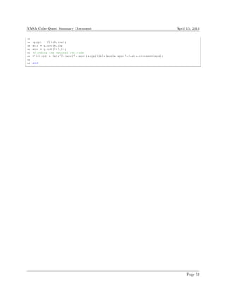
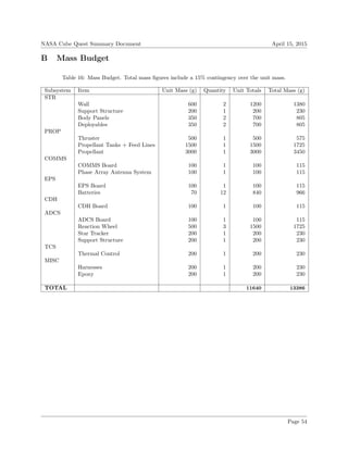
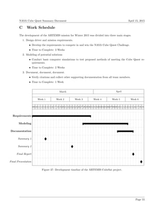
![NASA Cube Quest Summary Document April 15, 2015
References
[1] NASA CubeQuest Challenge Reference Materials. SLS Secondary Payload Trajectory.
www.nasa.gov/cubequest/reference/, January 2015.
[2] A.H.J. de Ruiter, C.J. Damaren, and J.R. Forbes. Spacecraft Dynamics and Control: An Introduction,
pages 183–188. Wiley, West Sussex, United Kingdom, 2013.
[3] Spaceflight Services. Launch Manifest Schedule.
http://spaceflightservices.com/manifest-schedule/, 2015.
[4] NASA CubeQuest Challenge Reference Materials. Cube Quest Challenge Operations and Rules.
www.nasa.gov/cubequest/reference/, January 2015.
[5] NASA CubeQuest Challenge Reference Materials. Required Navigation Artifacts for Authenticating
Claimed Communications Distances, and Verifying Achievement and Maintenance of Lunar Orbit for
Compliance with Cube Quest Challenge Rules. www.nasa.gov/cubequest/reference/, January 2015.
[6] Analytical Graphics Inc. Systems Tool Kit. http://www.agi.com/products/stk/, 2015.
[7] D. Folta et al. LunarCube Transfer Trajectory Options. In 25th
AAS/AIAA Space Flight Mechanics
Meeting, January 2015. http://engineering.purdue.edu/people/kathleen.howell.1/
Publications/Conferences/2015_AAS_FolDicClaHaaHow.pdf.
[8] J.P. Sheehan. Personal Communications, March 2015.
[9] M. Reardon, J. Yu, and C. Brandon. A Comparison of Low Cost Transfer Orbits from GEO to LLO
for a Lunar Cubesat Mission. In New Trends in Astrodynamics, June 2011. www.astrodynamics.eu/
Astrodynamics.eu/AstroconVI_Abstracts_and_Talks_files/Reardon-Talk.pdf.
[10] W.H. Michael and R.H. Tolson. Effect of Eccentricity of the Lunar Orbit, Oblateness of the Earth, and
Solar Gravitational Field on Lunar Trajectories. NASA, 1960.
[11] J Sellers et al. Understanding Space: An Introduction to Astronautics. McGraw Hill, 2004.
[12] T.I. Huque et al. Design and Performance Analysis of Microstrip Array Antennas with Optimum
Parameters for X-band Applications. International Journal of Advanced Computer Science and
Applications, 2(4):81–87, 2011. http://www.thesai.org/downloads/Volume2No4/Paper%
2013-Design%20and%20Performance%20Analysis%20of%20Microstrip%20Array%20Antennas%
20with%20Optimum%20Parameters%20for%20X-band%20Appli.pdf.
[13] N. Tucker. Matlab Phased Array Design Toolbox V2.5.
http://www.activefrance.com/Antennas/page22.html.
[14] D. Bapna, M. Martin, and W. Whittaker. Earth-Moon Communication from a Moving Lunar Rover.
Carnegie Mellon University Robotics Institute, 1996.
https://www.ri.cmu.edu/pub_files/pub1/bapna_deepak_1996_1/bapna_deepak_1996_1.pdf.
[15] J.R. Wertz, D.F. Everett, and J.J. Puschell. Space Mission Engineering: The New SMAD, page 637.
Space Technology Library, 2011.
[16] J. Berner. Deep Space Network Services Catalog. JPL, 820-001 Rev. F edition, February 2015.
https://deepspace.jpl.nasa.gov/files/dsn/820-100-F1.pdf.
[17] J.R. Wertz, D.F. Everett, and J.J. Puschell. Space Mission Engineering: The New SMAD, page 558.
Space Technology Library, 2011.
[18] J.R. Wertz, D.F. Everett, and J.J. Puschell. Space Mission Engineering: The New SMAD, page 562.
Space Technology Library, 2011.
Page 56](https://image.slidesharecdn.com/71722d65-e3b3-454a-aee6-5eab4a02991a-150717011219-lva1-app6891/85/Cube_Quest_Final_Report-62-320.jpg)
![NASA Cube Quest Summary Document April 15, 2015
[19] J.R. Wertz, D.F. Everett, and J.J. Puschell. Space Mission Engineering: The New SMAD, page 479.
Space Technology Library, 2011.
[20] C. Cagle. DSN Mission Service Interfaces, Policies, and Practices (MSIPP). JPL, 875-0001 Rev. G
edition, February 2015. https://deepspace.jpl.nasa.gov/files/dsn/875-0001-G1.pdf.
[21] Smith M.W. Pong, C.M. and M.W. Knutson. One-Arcsecond Line-of-Sight Pointing Control on
Exoplanetsat, a Three-Unit CubeSat. American Astronautical Society Guidance and Control
Conference, 2011.
http://ssl.mit.edu/exoplanetsat/wiki/images/8/8e/2011-02-06_AAS_GNC.pdf.
[22] Spectrolab Inc. Datasheet for 28.3% Ultra Triple Junction (UTJ) Solar Cells.
www.spectrolab.com/DataSheets/cells/PV%20UTJ%20Cell%205-20-10.pdf.
[23] A.H.J. de Ruiter, C.J. Damaren, and J.R. Forbes. Spacecraft Dynamics and Control: An Introduction,
pages 467–476. Wiley, West Sussex, United Kingdom, 2013.
[24] J.L. Crassidis and J.L. Junkins. Optimal Estimation of Dynamic Systems. CRC Press, Boca Raton,
FL, 2004.
[25] R. Mahony, T. Hamel, and J. Pflimlin. Nonlinear Complementary Filters on the Special Orthogonal
Group. IEEE Transactions on Automatic Control, 53(5):1203–1218, 2008.
[26] D.E. Zlotnik and J.R. Forbes. Rotation-Matrix-Based Attitude Control Without Angular Velocity
Measurements. In American Control Conference (ACC), 2014, pages 4931–4936, June 2014.
[27] A.H.J. de Ruiter and J.R. Forbes. General Identities for Parameterization of SO(3) with Applications.
ASME Journal of Applied Mechanics, 81:1–16, 2014.
[28] H. Hemmati. Laser-Communications with Lunar Cubesat.
www.lunar-cubes.com/docs/Hamid_Hemmati_13_04_11.pdf, 2013.
[29] Blue Canyon Technologies. XACT High-Performance Attitude Determination for Cubesats.
http://bluecanyontech.com/wp-content/uploads/2015/04/XACT-Data-Sheet.pdf.
[30] J.R. Wertz, D.F. Everett, and J.J. Puschell. Space Mission Engineering: The New SMAD, pages
395–407. Space Technology Library, 2011.
[31] L.E. Selva. Single-Event Gate Rupture and Single-Event Burnout Test Results Performed on Hi-Rel
Fuji Power MOSFETs: 2SK4217, 2SK4152, 2SK4155, and 2SK4158. JPL Publication, page 1, October
2009. https://nepp.nasa.gov/files/20287/09_163_5%20Selva_Scheick%20Single%20Event%
20Gate%20Rupture%20and%20Single%20Event%20Burnout%20Test%20Results%20on%20Hi%20Rel%
20Fuji%20Power%20MOSFETs%2009_26%2010_09%2011_17_09.pdf.
[32] Silva Co. Single Event Gate Rupture (SEGR) Simulations in a Power MOSFET. The Simulation
Standard, pages 10–12, January-March 2013. http://www.silvaco.com/tech_lib_TCAD/
simulationstandard/2013/jan_feb_mar/a2/jan_feb_mar2013_a2.pdf.
[33] G. Manyak. Fault Tolerant and Flexible CubeSat Software Architecture, June 2011.
http://polysat.calpoly.edu/download/Manyak_FSW_architecture.pdf.
[34] Planetary Systems Corporation. Canisterized Satellite Dispenser.
www.planetarysystemscorp.com/?post_type=product&p=448.
[35] Planetary Systems Corporation. Canisterized Satellite Dispenser (CSD) Data Sheet.
www.planetarysys.com/web/wp-content/uploads/2014/08/2002337B-CSD-Data-Sheet.pdf, July
2014. Version 2002337B.
[36] NASA CubeQuest Challenge Reference Materials. SLS Secondary Payload Users Guide (SPUG).
www.nasa.gov/cubequest/reference/, January 2015.
Page 57](https://image.slidesharecdn.com/71722d65-e3b3-454a-aee6-5eab4a02991a-150717011219-lva1-app6891/85/Cube_Quest_Final_Report-63-320.jpg)
![NASA Cube Quest Summary Document April 15, 2015
[37] Planetary Systems Corporation. Payload Specification for 3U, 6U, 12U, and 27U. www.planetarysys.
com/web/wp-content/uploads/2014/08/2002367B-Payload-Spec-for-3U-6U-12U-27U.pdf, July
2014. Version 2002367B.
[38] J.R. Wertz, D.F. Everett, and J.J. Puschell. Space Mission Engineering: The New SMAD, page 428.
Space Technology Library, 2011.
[39] J.R. Wertz, D.F. Everett, and J.J. Puschell. Space Mission Engineering: The New SMAD, page 434.
Space Technology Library, 2011.
[40] G. Diller. Space Shuttle Weather Launch Commit Criteria and KSC End of Mission Weather Landing
Criteria. www.nasa.gov/centers/kennedy/news/releases/2003/release-20030128.html, January
2003.
[41] G.R. Sharp and T.A. Loftin. Applications of High Thermal Conductivity Composites to Electronics
and Spacecraft Thermal Design.
http://ntrs.nasa.gov/archive/nasa/casi.ntrs.nasa.gov/19920015106.pdf, March 1990.
[42] D. Butler. NASA Technology Development Group Thermal Engineering Branch - Vary Emittance
Coatings. http://mscweb.gsfc.nasa.gov/545web/Groups/P2/Technology/VaryE.html, April 2012.
[43] Paragon Space Development Corporation. Variable Emissivity Radiator.
www.paragonsdc.com/brochures/VariableEmissivity_lo.pdf, October 2013.
[44] J. Cutler. Robust Orbit Determination: A Machine Learning Approach. In 12th
Annual CubeSat
Developers’ Workshop, April 2015. http://2ww.cubesat.org/index.php/workshops/
upcoming-workshops/132-2015-spring-cubesat-developers-workshop.
Page 58](https://image.slidesharecdn.com/71722d65-e3b3-454a-aee6-5eab4a02991a-150717011219-lva1-app6891/85/Cube_Quest_Final_Report-64-320.jpg)


