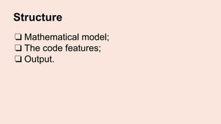
![The price of an Asian option by MCS
An Asian option (call) has discounted payoff:
Y = e-rT
[S - K]+
S =
1
m
S(ti )
i=1
m
å For fixed dates 0<t1<…<tm<T
Since for Monte Carlo simulation we describe the risk-neutral dynamics of the stock price, we
need to use the stochastic differential equation for modeling the price movement of the
underlying asset
S(T) = S(0)exp([r -
1
2
s 2
]T +sW(T))
Where W(T) is the random variable,
normally distributed with mean 0 and
variance T.](https://image.slidesharecdn.com/assignment15borisova-150306084810-conversion-gate01/85/The-Delta-Of-An-Arithmetic-Asian-Option-Via-The-Pathwise-Method-4-320.jpg)
![S(T) = S(0)exp([r -
1
2
s 2
]T +sW(T))
Monte Carlo simulation of the
lognormal asset price movement
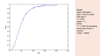
Model:
S = 100, r = 0.045, σ=15%,
trials = 100000
For fixed dates 0<t1<…<tm<T](https://image.slidesharecdn.com/assignment15borisova-150306084810-conversion-gate01/85/The-Delta-Of-An-Arithmetic-Asian-Option-Via-The-Pathwise-Method-5-320.jpg)

![Option value estimation and its
confidence level
The sample standard deviation
sC =
1
n-1
(Yi - ˆYn )2
i=1
n
å
1-δ quantile of the standard normal distribution zdConfidence interval:
ˆYn ± zd/2
sC
n
ˆYn =
1
n
Yi
1
n
å
E[ ˆYn ]= Y
ˆYn -Y
sC / n
Þ N(0,1)
The estimation of the option value is unbiased
As number of replications increases, the standardized estimator converges in
distribution to the standard normal](https://image.slidesharecdn.com/assignment15borisova-150306084810-conversion-gate01/85/The-Delta-Of-An-Arithmetic-Asian-Option-Via-The-Pathwise-Method-10-320.jpg)

The document discusses the computation of the delta of an arithmetic Asian option using Monte Carlo simulation and the pathwise method. It includes a detailed mathematical model, MATLAB code for simulations, and the estimation of option values and confidence intervals. The pathwise estimator is highlighted for its unbiased nature and efficiency in reducing variance and computational time compared to finite-difference methods.