Machine Learning & Linear
Regression
Faculty of Computing and
Information Technology
CPIS-703: Intelligent Information Systems
and
Decision Support
Department of Information Science
Machine Learning
- Grew out of work in AI
- New capability for computers
Examples:
- Database mining
Large datasets from growth of automation/web.
E.g., Web click data, medical records, biology,
engineering
- Applications can’t program by hand.
E.g., Autonomous helicopter, handwriting recognition, most
of Natural Language Processing (NLP), Computer Vision.
- Self-customizing programs
E.g., Amazon, Netflix product recommendations
- Understanding human learning (brain, real AI).
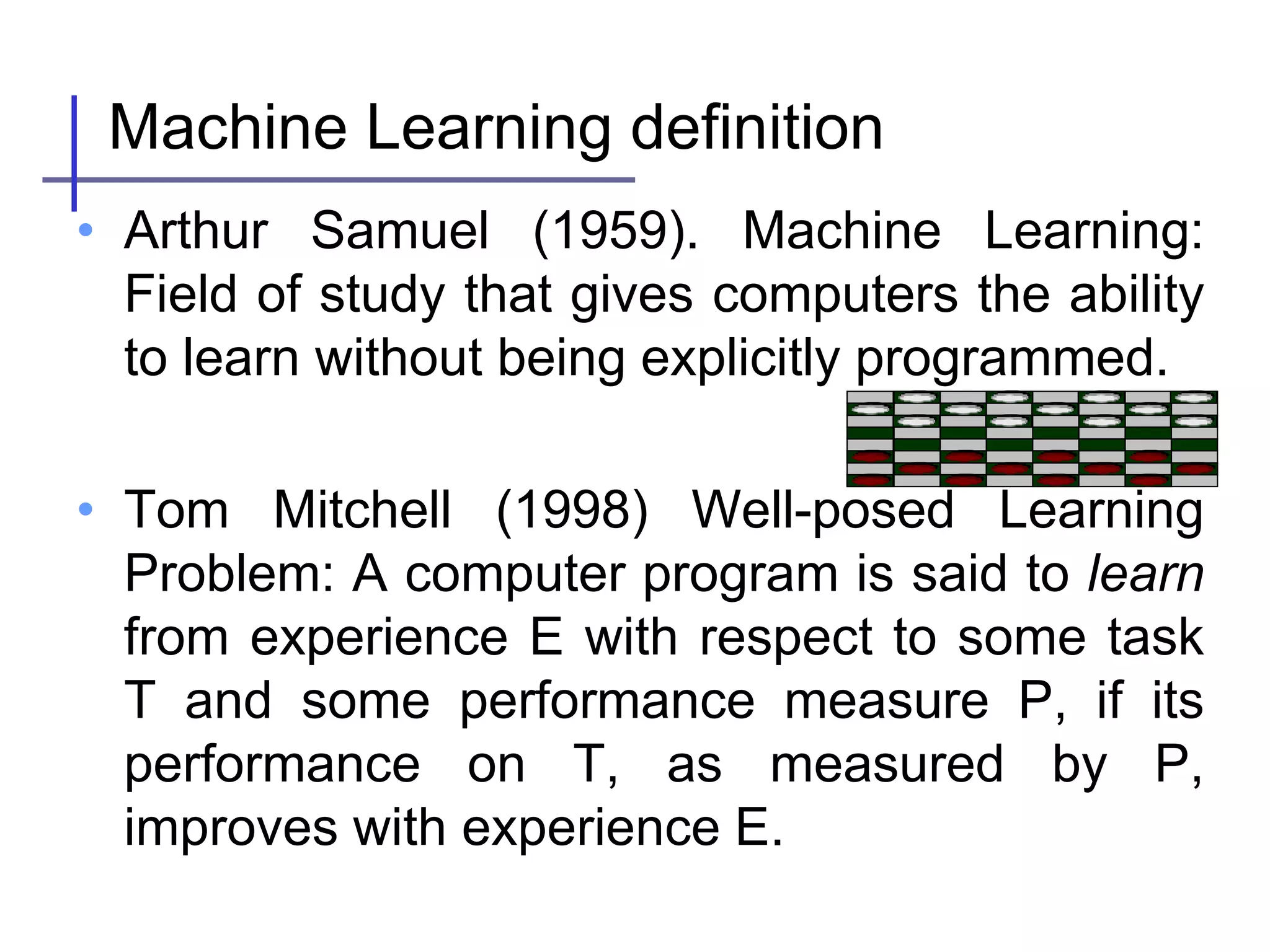
• Arthur Samuel (1959). Machine Learning:
Field of study that gives computers the ability
to learn without being explicitly programmed.
• Tom Mitchell (1998) Well-posed Learning
Problem: A computer program is said to learn
from experience E with respect to some task
T and some performance measure P, if its
performance on T, as measured by P,
improves with experience E.
Machine Learning definition
Classifying emails as spam or not spam.
Watching you label emails as spam or not spam.
The number (or fraction) of emails correctly classified as spam/not spam.
None of the above—this is not a machine learning problem.
Suppose your email program watches which emails you do or
do not mark as spam, and based on that learns how to better
filter spam. What is the task T in this setting?
“A computer program is said to learn from experience E with respect
to some task T and some performance measure P, if its performance
on T, as measured by P, improves with experience E.”
Machine learning algorithms:
- Supervised learning
- Unsupervised learning
Others: Reinforcement learning,
recommender systems.
Also talk about: Practical advice for applying
learning algorithms.
Machine learning Review
Supervised Learning
0
100
200
300
400
0 500 1000 1500 2000 2500
Housing price prediction
Price ($)
in 1000’s
Size in feet2
Regression: Predict
continuous valued
output (price)
Supervised Learning
“right answers” given
Cancer (malignant, benign)
Classification
Discrete
valued output
(0 or 1)
Malignant?
1(Y)
0(N)
Tumor Size
Tumor Size
Tumor Size
Age
- Clump Thickness
- Uniformity of Cell
Size
- Uniformity of Cell
Shape
…
Treat both as classification problems.
Treat problem 1 as a classification problem, problem 2 as a regression
problem.
Treat problem 1 as a regression problem, problem 2 as a classification
problem.
Treat both as regression problems.
You’re running a company, and you want to develop learning algorithms to address
each of two problems.
Problem 1: You have a large inventory of identical items. You want to predict how
many of these items will sell over the next 3 months.
Problem 2: You’d like software to examine individual customer accounts, and for
each account decide if it has been hacked/compromised.
Should you treat these as classification or as regression problems?
Unsupervised Learning
x1
x2
Supervised Learning
Unsupervised Learning
x1
x2
[Source: Daphne Koller]
Genes
Individuals
[Source: Daphne Koller]
Genes
Individuals
Organize computing clusters Social network analysis
Image credit: NASA/JPL-Caltech/E. Churchwell (Univ. of Wisconsin, Madison)
Astronomical data analysis
Market segmentation
Of the following examples, which would you address
using an unsupervised learning algorithm? (Check
all that apply.)
Given a database of customer data, automatically
discover market segments and group customers into
different market segments.
Given email labeled as spam/not spam, learn a spam
filter.
Given a set of news articles found on the web, group
them into set of articles about the same story.
Given a dataset of patients diagnosed as either having
diabetes or not, learn to classify new patients as having
diabetes or not.
Supervised learning
• Notation
– Features x
– Targets y
– Predictions ŷ
– Parameters q
Program (“Learner”)
Characterized by
some “parameters” θ
Procedure (using θ)
that outputs a prediction
Training data
(examples)
Features
Learning algorithm
Change θ
Improve performance
Feedback /
Target values Score performance
(“cost function”)
Linear regression
• Define form of function f(x) explicitly
• Find a good f(x) within that family
0 10 20
0
20
40
Target
y
Feature x
“Predictor”:
Evaluate line:
return r
More dimensions?
0
10
20
30
40
0
10
20
30
20
22
24
26
0
10
20
30
40
0
10
20
30
20
22
24
26
x1 x2
y
x1 x2
y
Notation
Define “feature” x0 = 1 (constant)
Then
Measuring error
0 20
0
Error or “residual”
Prediction
Observation
Mean squared error
• How can we quantify the error?
• Could choose something else, of course…
– Computationally convenient (more later)
– Measures the variance of the residuals
– Corresponds to likelihood under Gaussian model of “noise”
MSE cost function
• Rewrite using matrix form
(Matlab) >> e = y’ – th*X’; J = e*e’/m;
Visualizing the cost function
-1 -0.5 0 0.5 1 1.5 2 2.5 3
-40
-30
-20
-10
0
10
20
30
40
-1 -0.5 0 0.5 1 1.5 2 2.5 3
-40
-30
-20
-10
0
10
20
30
40
θ1
J(θ)
Supervised learning
• Notation
– Features x
– Targets y
– Predictions ŷ
– Parameters q
Program (“Learner”)
Characterized by
some “parameters” θ
Procedure (using θ)
that outputs a prediction
Training data
(examples)
Features
Learning algorithm
Change θ
Improve performance
Feedback /
Target values Score performance
(“cost function”)
Finding good parameters
• Want to find parameters which minimize our error…
• Think of a cost “surface”: error residual for that θ…
Linear regression: direct minimization
+
MSE Minimum
• Consider a simple problem
– One feature, two data points
– Two unknowns: µ0, µ1
– Two equations:
• Can solve this system directly:
• However, most of the time, m > n
– There may be no linear function that hits all the data exactly
– Instead, solve directly for minimum of MSE function
SSE (Sum of squared errors) Minimum
• Reordering, we have
• X (XT X)-1 is called the “pseudo-inverse”
• If XT is square and independent, this is the inverse
• If m > n: overdetermined; gives minimum MSE fit
Matlab SSE
• This is easy to solve in Matlab…
% y = [y1 ; … ; ym]
% X = [x1_0 … x1_m ; x2_0 … x2_m ; …]
% Solution 1: “manual”
th = y’ * X * inv(X’ * X);
% Solution 2: “mrdivide”
th = y’ / X’; % th*X’ = y => th = y/X’
“matrix-right-divide”
0 2 4 6 8 10 12 14 16 18 20
0
2
4
6
8
10
12
14
16
18
Effects of MSE choice
• Sensitivity to outliers
16 2 cost for this one datum
Heavy penalty for large errors
-20 -15 -10 -5 0 5
0
1
2
3
4
5
L1 error (minimum absolute error )
0 2 4 6 8 10 12 14 16 18 20
0
2
4
6
8
10
12
14
16
18 L2, original data
L1, original data
L1, outlier data
Cost functions for regression
“Arbitrary” functions can’t be
solved in closed form…
- use gradient descent
(MSE)
(MAE)
Something else entirely…
(???)
Linear regression: nonlinear features
+
Nonlinear functions
• What if our hypotheses are not lines?
– Ex: higher-order polynomials
0 2 4 6 8 10 12 14 16 18 20
0
2
4
6
8
10
12
14
16
18
Order 1 polynom ial
0 2 4 6 8 10 12 14 16 18 20
0
2
4
6
8
10
12
14
16
18
Order 3 polynom ial
Nonlinear functions
• Single feature x, predict target y:
• Sometimes useful to think of “feature transform”
Add features:
Linear regression in new features
Higher-order polynomials
• Fit in the same way
• More “features”
0 2 4 6 8 10 12 14 16 18 20
0
2
4
6
8
10
12
14
16
18
Order 1 polynom ial
0 2 4 6 8 10 12 14 16 18 20
-2
0
2
4
6
8
10
12
14
16
18
Order 2 polynom ial
0 2 4 6 8 10 12 14 16 18 20
0
2
4
6
8
10
12
14
16
18
Order 3 polynom ial
Features
• In general, can use any features we think are useful
• Other information about the problem
– Sq. footage, location, age, …
• Polynomial functions
– Features [1, x, x2, x3, …]
• Other functions
– 1/x, sqrt(x), x1 * x2, …
• “Linear regression” = linear in the parameters
– Features we can make as complex as we want!
Higher-order polynomials
• Are more features better?
• “Nested” hypotheses
– 2nd order more general than 1st,
– 3rd order “ “ than 2nd, …
• Fits the observed data better
Overfitting and complexity
• More complex models will always fit the training data
better
• But they may “overfit” the training data, learning
complex relationships that are not really present
X
Y
Complex model
X
Y
Simple model
Test data
• After training the model
• Go out and get more data from the world
– New observations (x,y)
• How well does our model perform?
Training data
New, “test” data
0 0.5 1 1.5 2 2.5 3 3.5 4 4.5 5
0
5
10
15
20
25
30
Training data
Training versus test error
• Plot MSE as a function
of model complexity
– Polynomial order
• Decreases
– More complex function
fits training data better
• What about new data?
Mean
squared
error
Polynomial order
New, “test” data
• 0th to 1st order
– Error decreases
– Underfitting
• Higher order
– Error increases
– Overfitting

06-01 Machine Learning and Linear Regression.pptx

  • 1.
    Machine Learning &Linear Regression Faculty of Computing and Information Technology CPIS-703: Intelligent Information Systems and Decision Support Department of Information Science
  • 2.
    Machine Learning - Grewout of work in AI - New capability for computers Examples: - Database mining Large datasets from growth of automation/web. E.g., Web click data, medical records, biology, engineering - Applications can’t program by hand. E.g., Autonomous helicopter, handwriting recognition, most of Natural Language Processing (NLP), Computer Vision.
  • 3.
    Machine Learning - Grewout of work in AI - New capability for computers Examples: - Database mining Large datasets from growth of automation/web. E.g., Web click data, medical records, biology, engineering - Applications can’t program by hand. E.g., Autonomous helicopter, handwriting recognition, most of Natural Language Processing (NLP), Computer Vision. - Self-customizing programs E.g., Amazon, Netflix product recommendations - Understanding human learning (brain, real AI).
  • 4.
    • Arthur Samuel(1959). Machine Learning: Field of study that gives computers the ability to learn without being explicitly programmed. • Tom Mitchell (1998) Well-posed Learning Problem: A computer program is said to learn from experience E with respect to some task T and some performance measure P, if its performance on T, as measured by P, improves with experience E. Machine Learning definition
  • 5.
    Classifying emails asspam or not spam. Watching you label emails as spam or not spam. The number (or fraction) of emails correctly classified as spam/not spam. None of the above—this is not a machine learning problem. Suppose your email program watches which emails you do or do not mark as spam, and based on that learns how to better filter spam. What is the task T in this setting? “A computer program is said to learn from experience E with respect to some task T and some performance measure P, if its performance on T, as measured by P, improves with experience E.”
  • 6.
    Machine learning algorithms: -Supervised learning - Unsupervised learning Others: Reinforcement learning, recommender systems. Also talk about: Practical advice for applying learning algorithms.
  • 7.
  • 16.
  • 17.
    0 100 200 300 400 0 500 10001500 2000 2500 Housing price prediction Price ($) in 1000’s Size in feet2 Regression: Predict continuous valued output (price) Supervised Learning “right answers” given
  • 18.
    Cancer (malignant, benign) Classification Discrete valuedoutput (0 or 1) Malignant? 1(Y) 0(N) Tumor Size Tumor Size
  • 19.
    Tumor Size Age - ClumpThickness - Uniformity of Cell Size - Uniformity of Cell Shape …
  • 20.
    Treat both asclassification problems. Treat problem 1 as a classification problem, problem 2 as a regression problem. Treat problem 1 as a regression problem, problem 2 as a classification problem. Treat both as regression problems. You’re running a company, and you want to develop learning algorithms to address each of two problems. Problem 1: You have a large inventory of identical items. You want to predict how many of these items will sell over the next 3 months. Problem 2: You’d like software to examine individual customer accounts, and for each account decide if it has been hacked/compromised. Should you treat these as classification or as regression problems?
  • 21.
  • 22.
  • 23.
  • 26.
  • 27.
  • 28.
    Organize computing clustersSocial network analysis Image credit: NASA/JPL-Caltech/E. Churchwell (Univ. of Wisconsin, Madison) Astronomical data analysis Market segmentation
  • 29.
    Of the followingexamples, which would you address using an unsupervised learning algorithm? (Check all that apply.) Given a database of customer data, automatically discover market segments and group customers into different market segments. Given email labeled as spam/not spam, learn a spam filter. Given a set of news articles found on the web, group them into set of articles about the same story. Given a dataset of patients diagnosed as either having diabetes or not, learn to classify new patients as having diabetes or not.
  • 30.
    Supervised learning • Notation –Features x – Targets y – Predictions ŷ – Parameters q Program (“Learner”) Characterized by some “parameters” θ Procedure (using θ) that outputs a prediction Training data (examples) Features Learning algorithm Change θ Improve performance Feedback / Target values Score performance (“cost function”)
  • 31.
    Linear regression • Defineform of function f(x) explicitly • Find a good f(x) within that family 0 10 20 0 20 40 Target y Feature x “Predictor”: Evaluate line: return r
  • 32.
  • 33.
  • 34.
    Measuring error 0 20 0 Erroror “residual” Prediction Observation
  • 35.
    Mean squared error •How can we quantify the error? • Could choose something else, of course… – Computationally convenient (more later) – Measures the variance of the residuals – Corresponds to likelihood under Gaussian model of “noise”
  • 36.
    MSE cost function •Rewrite using matrix form (Matlab) >> e = y’ – th*X’; J = e*e’/m;
  • 37.
    Visualizing the costfunction -1 -0.5 0 0.5 1 1.5 2 2.5 3 -40 -30 -20 -10 0 10 20 30 40 -1 -0.5 0 0.5 1 1.5 2 2.5 3 -40 -30 -20 -10 0 10 20 30 40 θ1 J(θ)
  • 38.
    Supervised learning • Notation –Features x – Targets y – Predictions ŷ – Parameters q Program (“Learner”) Characterized by some “parameters” θ Procedure (using θ) that outputs a prediction Training data (examples) Features Learning algorithm Change θ Improve performance Feedback / Target values Score performance (“cost function”)
  • 39.
    Finding good parameters •Want to find parameters which minimize our error… • Think of a cost “surface”: error residual for that θ…
  • 40.
  • 41.
    MSE Minimum • Considera simple problem – One feature, two data points – Two unknowns: µ0, µ1 – Two equations: • Can solve this system directly: • However, most of the time, m > n – There may be no linear function that hits all the data exactly – Instead, solve directly for minimum of MSE function
  • 42.
    SSE (Sum ofsquared errors) Minimum • Reordering, we have • X (XT X)-1 is called the “pseudo-inverse” • If XT is square and independent, this is the inverse • If m > n: overdetermined; gives minimum MSE fit
  • 43.
    Matlab SSE • Thisis easy to solve in Matlab… % y = [y1 ; … ; ym] % X = [x1_0 … x1_m ; x2_0 … x2_m ; …] % Solution 1: “manual” th = y’ * X * inv(X’ * X); % Solution 2: “mrdivide” th = y’ / X’; % th*X’ = y => th = y/X’ “matrix-right-divide”
  • 44.
    0 2 46 8 10 12 14 16 18 20 0 2 4 6 8 10 12 14 16 18 Effects of MSE choice • Sensitivity to outliers 16 2 cost for this one datum Heavy penalty for large errors -20 -15 -10 -5 0 5 0 1 2 3 4 5
  • 45.
    L1 error (minimumabsolute error ) 0 2 4 6 8 10 12 14 16 18 20 0 2 4 6 8 10 12 14 16 18 L2, original data L1, original data L1, outlier data
  • 46.
    Cost functions forregression “Arbitrary” functions can’t be solved in closed form… - use gradient descent (MSE) (MAE) Something else entirely… (???)
  • 47.
  • 48.
    Nonlinear functions • Whatif our hypotheses are not lines? – Ex: higher-order polynomials 0 2 4 6 8 10 12 14 16 18 20 0 2 4 6 8 10 12 14 16 18 Order 1 polynom ial 0 2 4 6 8 10 12 14 16 18 20 0 2 4 6 8 10 12 14 16 18 Order 3 polynom ial
  • 49.
    Nonlinear functions • Singlefeature x, predict target y: • Sometimes useful to think of “feature transform” Add features: Linear regression in new features
  • 50.
    Higher-order polynomials • Fitin the same way • More “features” 0 2 4 6 8 10 12 14 16 18 20 0 2 4 6 8 10 12 14 16 18 Order 1 polynom ial 0 2 4 6 8 10 12 14 16 18 20 -2 0 2 4 6 8 10 12 14 16 18 Order 2 polynom ial 0 2 4 6 8 10 12 14 16 18 20 0 2 4 6 8 10 12 14 16 18 Order 3 polynom ial
  • 51.
    Features • In general,can use any features we think are useful • Other information about the problem – Sq. footage, location, age, … • Polynomial functions – Features [1, x, x2, x3, …] • Other functions – 1/x, sqrt(x), x1 * x2, … • “Linear regression” = linear in the parameters – Features we can make as complex as we want!
  • 52.
    Higher-order polynomials • Aremore features better? • “Nested” hypotheses – 2nd order more general than 1st, – 3rd order “ “ than 2nd, … • Fits the observed data better
  • 53.
    Overfitting and complexity •More complex models will always fit the training data better • But they may “overfit” the training data, learning complex relationships that are not really present X Y Complex model X Y Simple model
  • 54.
    Test data • Aftertraining the model • Go out and get more data from the world – New observations (x,y) • How well does our model perform? Training data New, “test” data
  • 55.
    0 0.5 11.5 2 2.5 3 3.5 4 4.5 5 0 5 10 15 20 25 30 Training data Training versus test error • Plot MSE as a function of model complexity – Polynomial order • Decreases – More complex function fits training data better • What about new data? Mean squared error Polynomial order New, “test” data • 0th to 1st order – Error decreases – Underfitting • Higher order – Error increases – Overfitting