Spark Streaming allows processing live data streams using small batch sizes to provide low latency results. It provides a simple API to implement complex stream processing algorithms across hundreds of nodes. Spark SQL allows querying structured data using SQL or the Hive query language and integrates with Spark's batch and interactive processing. MLlib provides machine learning algorithms and pipelines to easily apply ML to large datasets. GraphX extends Spark with an API for graph-parallel computation on property graphs.

1. Apache Spark Components
Spark Streaming | Spark SQL | MLlib | GraphX
Girish Khanzode

2. Contents
• Spark Streaming
– Micro batch
– Stateful Stream Processing
– DStream
– Socket Stream
– File Stream
• Spark SQL
– DataFrame
– DataFrameAPI
– Supported Data Formats and Sources
– Plan Optimization & Execution
– Rules Based Optimization
• MLlib
– Algorithms
– Key Features
– Pipeline
• GraphX
– PropertyGraph
– GraphViews
– TripletView
– Subgraph
– DistributedGraph Representation
• Graph Algorithms
• References

3. Spark Streaming
A framework for large scale stream processing

4. Spark Streaming

5. Spark Streaming
• Extends Spark for big data stream processing
• Efficient, fault-tolerant, stateful stream processing of live stream data
• Integrates with Spark’s batch and interactive processing
• Scales to hundreds of nodes
• Can achieve latencies on scale of seconds

6. Spark Streaming
• Can absorb live data streams from Kafka, Flume, ZeroMQ etc
• Simple Batch likeAPI to implement complex algorithms
• Integrates with other Spark extensions
• Started in 2012, alpha released with Spark 0.7 in 2013, released with Spark
0.9 in 2014

7. Need for Spark Streaming
• Existing frameworks can either
– Stream process 100s of MBs with low latency
– Batch processTBs of data with high latency
• Painful to maintain two different stacks
– Different programming models
– Doubles implementation effort

8. Need for Spark Streaming
• Many applications must process large streams of live data and provide
results in near-real-time
– Social network trends
– Website statistics
– Intrusion detection systems
• Many environments require processing same data in live streaming as
well as batch post-processing

9. Micro batch
• Spark streaming is a fast batch processing system
• Spark streaming collects stream data into small batch and runs batch
processing on it
• Batch can be as small as 1 second to as big as multiple hours
• Spark job creation and execution overhead is so low it can do all that
under a second
• These batches are called as DStreams

10. Stateful Stream Processing
• Traditional streaming systems have a event-driven record-at-a-time
processing model
– Each node has mutable state
– For each record, update state & send new records
• State is lost if node dies
• Making stateful stream processing fault-tolerant is a challenge

11. Stateful Stream Processing

12. Streaming System - Storm
• Replays record if not processed by a node
• Processes each record at least once
• May update mutable state twice
• Mutable state can be lost due to failure

13. Streaming System -Trident
• Uses transactions to update state
• Processes each record exactly once
• Per state transaction updates slow

14. Spark Streaming
• Runs a streaming computation as a series of very small deterministic
batch jobs
• Splits the live stream into batches of X seconds
• Spark treats each batch of data as RDDs and processes them using RDD
operations
• Processed results of RDD operations are returned in batches

15. High LevelView

16. Spark Streaming
• Runs as a series of small (~1 s) batch jobs, keeping state in memory as
fault-tolerant RDDs
• Batch sizes as low as 0.5 second, latency ~ 1 second
• Potential for combining batch processing and streaming processing in the
same system
• Result: can process 42 million records/second (4 GB/s) on 100 nodes at
sub-second latency

17. Spark Streaming
• tweetStream
• .flatMap(_.toLower.split)
• .map(word => (word, 1))
.reduceByWindow(“5s”, _ + _)
T=1
T=2
…
map reduceByWindow

18. Streaming
• Creates RDDs from stream source on a defined interval
• Same operation as normal RDDs
• Supports a variety of sources
• Exactly once message guarantee

19. Discretized Stream - DStream
• Basic abstraction provided by Spark Streaming
• Input stream is divided into multiple discrete batches
• Represents a stream of data
• Implemented as a sequence of RDDs
• Each batch of DStream is represented as RDD
underneath

20. Discretized Stream - DStream
• These RDD are replicated in cluster for fault tolerance
• Every DStream operation results in RDD transformation
• APIs provided to access these RDD is directly
• Can combine stream and batch processing
• Configurable intervals - 1 second, 5 second, 5 minutes
etc.

21. Discretized Stream - DStream

22. DStream transformation
• val ssc = new StreamingContext(args(0),
"wordcount", Seconds(5))
• val lines =
ssc.socketTextStream("localhost",50050)
• val words = lines.flatMap(_.split(" "))

23. Socket Stream
• Ability to listen to any socket on remote machines
• Need to configure host and port
• Both Raw andText representation of socket available
• Built in retry mechanism

24. File Stream
• Allows tracking new files in a given directory on HDFS
• Whenever there is new file appears, spark streaming will pick it up
• Only works for new files, modification for existing files will not be
considered
• Tracked using file creation time

25. ReceiverArchitecture

26. Stateful Operations
• Ability to maintain random state across multiple batches
• Fault tolerant
• Exactly once semantics
• WAL (Write Ahead Log) for receiver crashes

27. How Stateful OperationsWork?
• Generally state is a mutable operation
• But in functional programming, state is represented with state machine
going from one state to another
• fn(oldState,newInfo) => newState
• In Spark, state is represented using RDD
• Change in the state is represented using transformation of RDD’s
• Fault tolerance of RDD helps in fault tolerance of state

28. Transform API
• In stream processing, ability to combine stream data with batch data is
extremely important
• Both batch API and stream API share RDD as abstraction
• TransformAPI of DStream allows us to access underneath RDD’s directly
• Example - Combine customer sales data with customer information

29. Window Based Operations

30. DStream Inputs
• DStream is Created from
– streaming input sources
– applying transformations on existing DStreams
• Basic input sources
– Built-in - file system, socket
– Non-built in -Avro, CSV …
– Unreliable
Ingest Transform Output

31. DStream Inputs
• Advanced input sources
– Twitter, Kafka, Flume, Kinesis, MQTT, ….
– Need external library
– Reliable or unreliable
• Custom input Dstream - Implement two classes
– Input DStream
– Receiver
• Reliable Receiver
• Unreliable Receiver

32. DStream Creation viaTransformation
• Data collected, buffered and replicated by receiver (one per DStream) and then
pushed to a stream as small RDDs
• Transformations modify data from one DStream to another
• Classifications
– Standard RDD operations – map, countByValue, reduceByKey, join,…
– Stateful operations – window, updateStateByKey, transform,
countByValueAndWindow, …

33. DStream Creation viaTransformation

34. Comparison with Storm
• Higher throughput than Storm
– Spark Streaming - 670k records/sec/node
– Storm - 115k records/sec/node
– Commercial systems: 100-500k records/sec/node
Throughputpernode
(MB/s)
Record Size (bytes)
WordCount
Spark
Storm
Throughputpernode
(MB/s)
Record Size (bytes)
Grep
Spark
Storm

35. SPARK SQL
Apache Spark Data Access

36. Spark SQL
• Part of the core distribution since Spark 1.0 (April 2014)
• Integrated with the Spark stack
• Supports querying data either via SQL or via the Hive Query Language
• Originated as the Apache Hive port to run on top of Spark (in place of MapReduce)
• Can weave SQL queries with code transformations

37. Spark SQL
• Capability to expose Spark datasets over JDBC API and allow running the SQL like
queries on Spark data using traditional BI and visualization tools
• Allows to ETL their data from different formats like JSON, Parquet or a Database,
transform it, and expose it for ad-hoc querying
• Bindings in Python, Scala, and Java

38. Spark SQL

39. Spark SQL

40. SQL Access to Structured Data
• Existing RDDs
• Hive warehouses (uses existing metastore, SerDes and UDFs)
• JDBC/ODBC - use existing BI tools to query large datasets

41. DataFrame
• A distributed collection of data rows organized into named columns
• An abstraction for selection, filter, aggregate and plot structured data
• Conceptually equivalent to a table in a relational database or a data frame
in R/Python, but with richer optimizations under the hood
• Constructed from sources
– Structured data files
– Hive tables
– External databases
– Existing RDDs

42. DataFrame Internals
• Internally represented as a logical plan
• Lazy execution - computation only happens when an action (display
result, save output) is required
– Allows executions to be optimized by applying techniques such as predicate
push-downs and bytecode generation
• All DataFrame operations are also automatically parallelized and
distributed on clusters

43. DataFrame Construction - Python code
• # Construct a DataFrame from the users table in Hive
– users = context.table("users")
• # from JSON files in S3
– logs = context.load("s3n://path/to/data.json", "json")
• DataFrames provide a domain-specific language for distributed data
manipulation

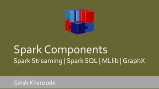
44. Using DataFrames
• # Create a new DataFrame that contains “young users” only
– young = users.filter(users.age < 21)
• # Alternatively, using Pandas-like syntax
– young = users[users.age < 21]
• # Increment everybody’s age by 1
– young.select(young.name, young.age + 1)

45. Using DataFrames
• # Count the number of young users by gender
– young.groupBy("gender").count()
• # Join young users with another DataFrame called logs
– young.join(logs, logs.userId == users.userId, "left_outer")
• #SQL using Spark SQL - Count number of users in the young DataFrame
– young.registerTempTable("young")
– context.sql("SELECT count(*) FROM young")

46. Spark and Pandas - Conversion
• # Convert Spark DataFrame to Pandas
– pandas_df = young.toPandas()
• # Create a Spark DataFrame from Pandas
– spark_df = context.createDataFrame(pandas_df)

47. DataFrame API
• Common operations can be expressed as calls to the DataFrameAPI
– Selecting required columns
– Joining different data sources
– Aggregation (count, sum, average, etc)
– Filtering

48. Supported Data Formats and Sources
1. JSON files
2. Parquet files
3. Hive tables
4. Local file systems
5. Distributed file systems (HDFS)
6. Cloud storage (S3)
7. External RDBMS via JDBC
8. Extend DataFrames through Spark
SQL’s external data sources API to
support any third-party data formats
or sources
9. Existing third-party extensions - Avro,
CSV, ElasticSearch, and Cassandra

49. Combine Multiple Sources
• Join a site’s textual traffic log stored in S3 with a PostgreSQL database to
count the number of times each user has visited the site
– users = context.jdbc("jdbc:postgresql:production", "users")
– logs = context.load("/path/to/traffic.log")
– logs.join(users, logs.userId == users.userId, "left_outer") .groupBy("userId").agg({"*":
"count"})

50. Automatic Mechanisms to Read Less Data
• Converting to more efficient formats
• Using columnar formats (parquet)
• Using partitioning (/year=2014/month=02/…)
• Skipping data using statistics (min, max...)
• Pushing predicates into storage systems (JDBC)

51. Intelligent Optimization and Code Generation
• DataFrames in Spark have their execution automatically optimized by a
query optimizer
• Before any computation on a DataFrame starts, the Catalyst optimizer
compiles the operations that were used to build the DataFrame into a
physical plan for execution
• Because the optimizer understands the semantics of operations and
structure of the data, it can make intelligent decisions to speed up
computation

52. Intelligent Optimization and Code Generation
• At a high level, there are two types of optimizations
• Catalyst applies logical optimizations such as predicate pushdown
• The optimizer can push filter predicates down into the data source,
enabling the physical execution to skip irrelevant data
• In the case of Parquet files, entire blocks can be skipped and comparisons
on strings can be turned into cheaper integer comparisons via dictionary
encoding

53. Intelligent Optimization and Code Generation
• In the case of relational databases, predicates are pushed down into the
external databases to reduce the amount of data traffic
• Catalyst compiles operations into physical plans for execution and
generates JVM bytecode for those plans that is often more optimized
than hand-written code
• It can choose intelligently between broadcast joins and shuffle joins to
reduce network traffic

54. Intelligent Optimization and Code Generation
• It can also perform lower level optimizations such as eliminating
expensive object allocations and reducing virtual function calls
• Performance improvements for existing Spark programs when they
migrate to DataFrames
• Since the optimizer generates JVM bytecode for execution, Python users
experience the same high performance as Scala and Java users

55. Plan Optimization & Execution
DataFrames and SQL share the same
optimization/execution pipeline

56. SQL Execution Plans
• Logical and Physical query plans
– Both are trees representing query evaluation
– Internal nodes are operators over the data
– Logical plan is higher-level and algebraic
– Physical plan is lower-level and operational
• Logical plan operators
– Correspond to query language constructs
– Conceptually describe what operation needs to be performed
• Physical plan operators
– Correspond to implemented access methods
– Physically Implement the operation described by logical operators
Binding & Analyzing
Unresolved Logical
Plan
Logical Plan
SQLText
Optimized Logical
Plan
Physical Plan
Parsing
Optimizing
Query Planning

57. Query Example
SELECT name
FROM (
SELECT id, name
FROM people ) p
WHERE p.id = 1

58. Naive Query Planning
SELECT name
FROM (
SELECT id, name
FROM people ) p
WHERE p.id = 1

59. Optimized Execution
• Writing imperative code to optimize
all possible patterns is hard
• Instead opt for simpler rules
– Each rule makes single change
– Run multiple rules together to
fixed points

60. Rules Based Optimization

61. Performance Comparison

62. MLLIB
Apache Spark Machine Learning Library

63. MLlib

64. Algorithms

65. Key Features
• Low level library in Spark
• Built-in data analysis workflow
• Free performance gains
• Scalable
• Python, Scala, JavaAPIs
• Broad coverage of applications & algorithms
• Rapid improvements in speed & robustness
• Easy to use
• Integrated workflow

66. Functionality
• Classes for common operations
• Scaling, normalization, statistical summary, correlation …
• Numeric RDD operations, sampling …
• Random generators
• Words extractions (TF-IDF)
– generating feature vectors from text documents / web pages

67. Speed Improvements

68. Sample Code

69. Linear Regression Example
• Method run() trains model
• Parameters are set with setters setNumInterations and setIntercept
• Stochastic Gradient Descent (SGD) algorithm is used for minimizing function

70. Typical MLWorkflow

71. Pipeline API
• Pipeline is a series of algorithms (feature transformation, model fitting, ...)
• Easy workflow construction
• Distribution of parameters into each stage
• MLlib is easier to use
• Uses uniform dataset representation - SchemaRDD from SparkSQL
– multiple named columns (similar to SQL table)

72. Pipeline

73. GRAPHX
Apache Spark GraphAPI

74. Graphs are Everywhere
• Social Networks
• Web Graphs
• User-Item Graphs

75. GraphX
• New API that blurs distinction between graphs and tables
• Unifies data-parallel and graph-parallel systems
• SparkAPI for graphs
– Web-Graphs and Social Networks
– graph-parallel computation like PageRank and Collaborative Filtering

76. GraphX
• Extends Spark RDD abstraction using Resilient Distributed Property
Graph - a directed multi-graph with properties attached to each vertex
and edge
• Exposes fundamental operators like subgraph, joinVertices, and
mapReduceTriplets for graph computation
• Includes graph algorithms and builders for graph analytics tasks

77. Cross-World Manipulation Enabling

78. Unifying Data-Parallel and Graph-Parallel Analytics
• Tables and Graphs are composable views of the same physical data
• Each view has its own operators that exploit the semantics of the view to
achieve efficient execution

79. Property Graph
• A directed graph with potentially multiple parallel edges sharing the
same source and destination vertex with properties attached to each
vertex and edge
• Each vertex is keyed by a unique 64-bit long identifier (VertexID)
• Edges have corresponding source and destination vertex identifiers
• Properties are stored as Scala/Java objects with each edge and vertex in
the graph

80. Property Graph
• Vertex Property
– User Profile
– Current PageRank Value
• Edge Property
– Weights
– Relationships
– Timestamps

81. Property Graph
• Constructed from raw files, RDDs and synthetic generators
• Immutable, distributed, and fault-tolerant
• Changes to the values or structure of the graph are accomplished by producing a
new graph with the desired changes
• Parts of the original graph (unaffected structure, attributes, and indices) are
reused in the new graph
• Each partition of the graph can be recreated on a different machine in the event
of a failure
• Represented using two Spark RDDs
– Edge collection:VertexRDD
– Vertex collection: EdgeRDD

82. GraphViews
• Graph class contains members graph.vertices and graph.edges to access
the vertices and edges of the graph
• These members extend RDD[(VertexId,V)] and RDD[Edge[E]]
• Are backed by optimized representations that leverage the internal
GraphX representation of graph data

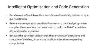
83. TripletView
• Triplets operator joins vertices and edges
• Logically joins the vertex and edge properties yielding an RDD[EdgeTriplet[VD,
ED]] containing instances of the EdgeTriplet class
• This join is graphically expressed as

84. TripletView

85. Subgraph
• Operator that takes vertex and edge predicates and returns the graph
containing only the vertices that satisfy the vertex predicate (evaluate to
true) and edges that satisfy the edge predicate and connect vertices that
satisfy the vertex predicate

86. Distributed Graph Representation
• Representing graphs using two RDDs
– edge-collection
– Vertex-collection
• Vertex-cut partitioning

87. Distributed Graph Representation

88. Distributed Graph Representation
• Each vertex partition contains a bitmask and routing table
• Routing table - a logical map from a vertex id to the set of edge partitions
that contains adjacent edges
• Bitmask - enables the set intersection and filtering
– Vertices bitmasks are updated after each operation (mapReduceTriplets)
– Vertices hidden by the bitmask do not participate in the graph operations

89. Graph Algorithms
• Collaborative Filtering
– Alternating Least Squares
– Stochastic Gradient Descent
– Tensor Factorization
• Structured Prediction
– Loopy Belief Propagation
– Max-Product Linear
• Programs
– Gibbs Sampling
• Semi-supervised ML
– Graph SSL
– CoEM
• Community Detection
– Triangle-Counting
– K-core Decomposition
– K-Truss
• Graph Analytics
– PageRank
– Personalized PageRank
– Shortest Path
– GraphColoring
• Classification
– Neural Networks

90. References
1. http://spark.apache.org/graphx
2. http://spark.apache.org/streaming/
3. http://spark-summit.org/wp-content/uploads/2014/07/Performing-Advanced-Analytics-on-Relational-Data-with-Spark-SQL-
Michael-Armbrust.pdf
4. http://web.stanford.edu/class/cs346/qpnotes.html
5. https://github.com/apache/spark/tree/master/sql
6. Resilient Distributed Datasets: A Fault-Tolerant Abstraction for In-Memory Cluster Computing. Matei Zaharia, Mosharaf
Chowdhury. Technical Report UCB/EECS-2011-82. July 2011
7. M. Zaharia, T. Das, H. Li, T. Hunter, S. Shenker, and I. Stoica. Discretized Streams: Fault-Tolerant Streaming Computation at Scale,
SOSP 2013, November 2013
8. K. Ousterhout, P. Wendell, M. Zaharia and I. Stoica. Sparrow: Distributed, Low-Latency Scheduling, SOSP 2013, November 2013
9. R. Xin, J. Rosen, M. Zaharia, M. Franklin, S. Shenker, and I. Stoica. Shark: SQL and Rich Analytics at Scale, SIGMOD 2013, June 2013
10. A. Ghodsi, M. Zaharia, B. Hindman, A. Konwinski, S. Shenker, and I. Stoica, Dominant Resource Fairness: Fair Allocation of Multiple
Resources Types, NSDI 2011, March 2011
11. Spark: In-Memory Cluster Computing for Iterative and Interactive Applications, Stanford University, Stanford, CA, February 2011

91. ThankYou
Visit My LinkedIn Profile
https://in.linkedin.com/in/girishkhanzode