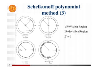
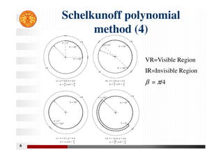
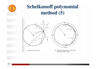
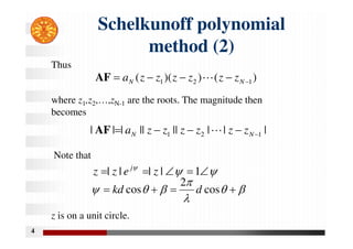
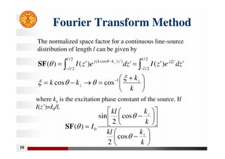
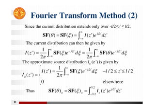
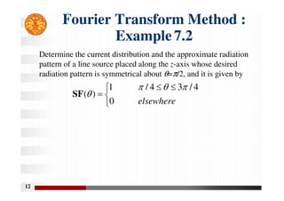
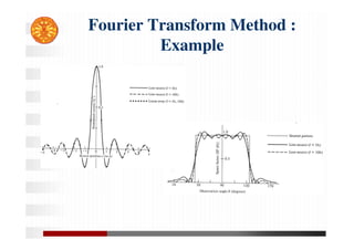
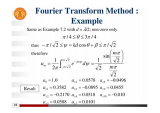
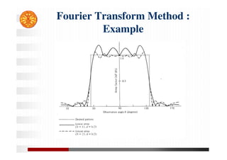
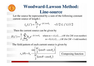
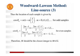
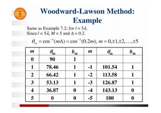
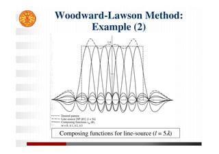
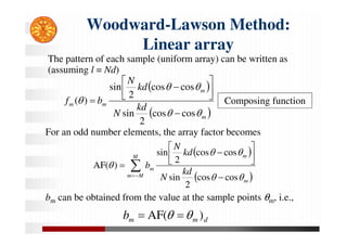
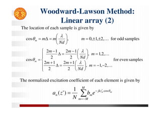
This document discusses various methods for antenna synthesis including: 1) The Schelkunoff polynomial method which represents the array factor as a polynomial and uses roots to determine the pattern. 2) The Fourier transform method which approximates a continuous source distribution as a discrete array and determines excitation coefficients from the desired pattern. 3) The Woodward-Lawson method which samples a desired pattern and represents the total pattern as a finite sum of composing functions to synthesize the pattern. 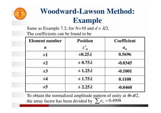It provides examples of applying these methods to design linear arrays with specific radiation patterns.

1. 1
Chapter 7 : Antenna Synthesis
• Continuous sources vs. Discrete sources
• Schelkunoff polynomial method
• Fourier transform method
• Woodward-Lawson method
• Triangular, cosine and cosine-squared
amplitude distributions

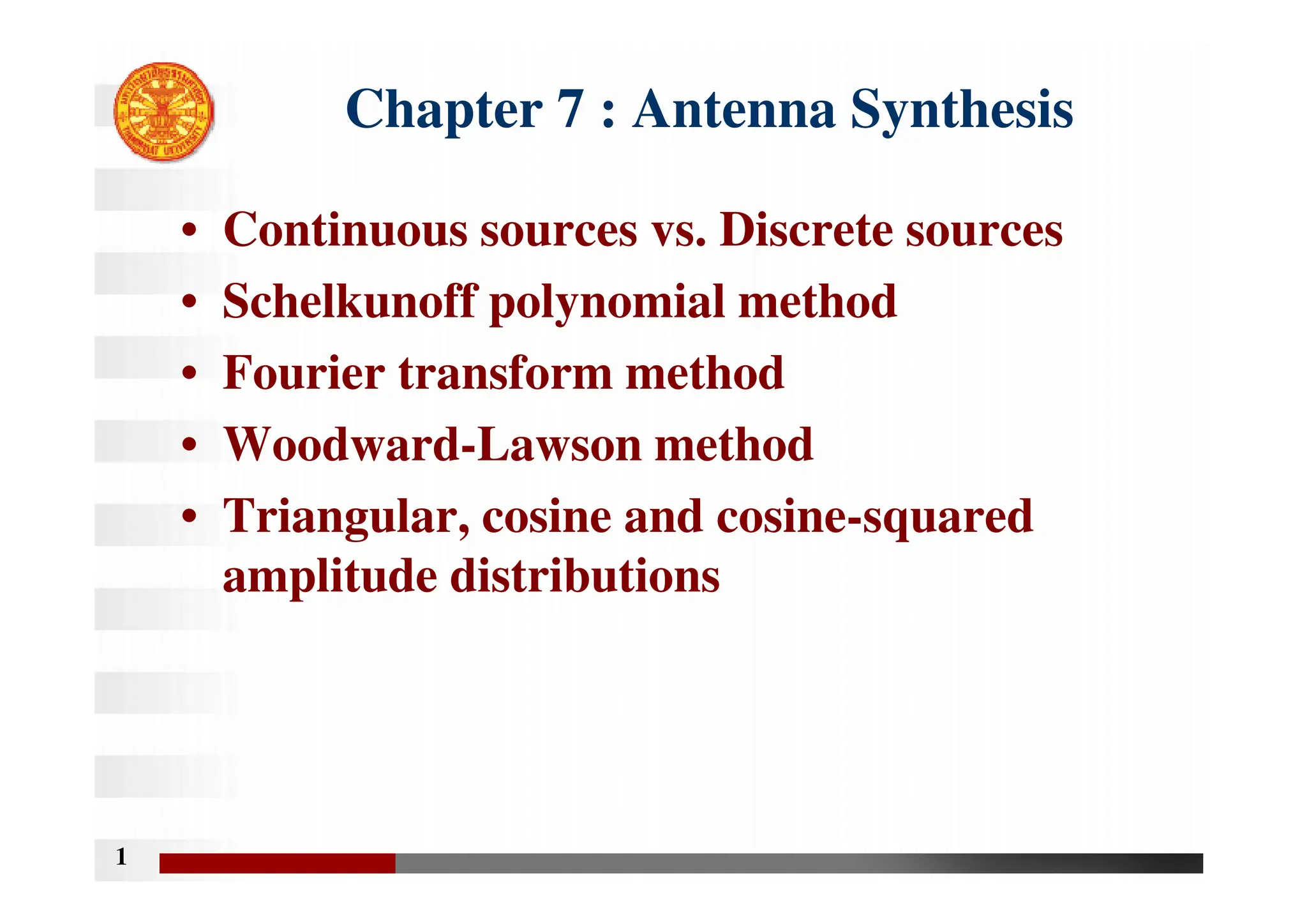
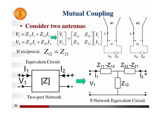
2. 2
Continuous sources
Recall the array factor
If the number of elements increases in a fixed-length array,
the source approaches a continuous distribution.
In the limit, the array factor becomes the space factor, i.e.,






N
n
n
j
n kd
e
a
1
)
1
(
cos
; 



AF
)
'
(
)
1
(
)
'
( z
j
n
n
j
n
n
e
z
I
e
a 



The radiation characteristics of continuous sources can
be approximated by discrete-element arrays, i.e.,



2
/
2
/
)]
'
(
cos
'
[
'
)
'
(
l
l
z
kz
j
n dz
e
z
I n


SF

3. 3
Schelkunoff polynomial
method
)
cos
( 

 



 kd
j
j
e
e
jy
x
z
The array factor for an N-element, equally spaced, non-
uniform amplitude, and progressive phase excitation is given
by
Let






N
n
n
j
n kd
e
a
1
)
1
(
cos
; 



AF









N
n
N
N
n
n z
a
z
a
a
z
a
1
1
2
1
1
L
AF
which is a polynomial of degree (N-1).

4. 4
Schelkunoff polynomial
method (2)







 1
|
|
|
| z
e
z
z j
Thus
Note that
)
(
)
)(
( 1
2
1 



 N
N z
z
z
z
z
z
a L
AF






 


 cos
2
cos d
kd
z is on a unit circle.
where z1,z2,…,zN-1 are the roots. The magnitude then
becomes
|
|
|
||
||
|
|
| 1
2
1 



 N
N z
z
z
z
z
z
a L
AF

5. Schelkunoff polynomial
method (3)
5
VR=Visible Region
IR=Invisible Region
β = 0

6. Schelkunoff polynomial
method (4)
6
VR=Visible Region
IR=Invisible Region
β = π/4

7. Schelkunoff polynomial
method (5)
7

8. Schelkunoff polynomial
method : Example
8
Design a linear array with a spacing between the elements
of d=λ/4 such that it has zeros at θ=0,π/2,π. Determine the
number of elements, their excitation, and plot the derived
pattern.

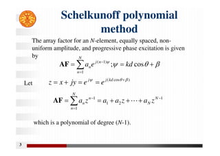
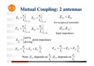
9. Schelkunoff polynomial
method : Example pattern
9
0 20 40 60 80 100 120 140 160 180
−50
−45
−40
−35
−30
−25
−20
−15
−10
−5
0
θ [Degree]
|(AF)
n
|
[dB]
4−element array factor

10. Fourier Transform Method
10
The normalized space factor for a continuous line-source
distribution of length l can be given by





 












k
k
k
k
dz
e
z
I
dz
e
z
I
z
z
l
l
z
j
l
l
z
k
k
j z




 

1
2
/
2
/
'
2
/
2
/
)
'
)
cos
(
cos
cos
'
)
'
(
'
)
'
(
)
(
SF
where kz is the excitation phase constant of the source. If
I(z’)=I0/l,





















k
k
kl
k
k
kl
I
z
z



cos
2
cos
2
sin
)
( 0
SF

11. Fourier Transform Method (2)
11
Since the current distribution extends only over -l/2≤z’≤ l/2,





 '
)
'
(
)
(
)
( '
dz
e
z
I z
j

 SF
SF
The approximate source distribution Ia (z’) is given by











 







d
e
d
e
z
I z
j
z
j '
'
)
(
2
1
)
(
2
1
)
'
( SF
SF
The current distribution can then be given by









 




elsewhere
0
2
/
'
2
/
)
(
2
1
)
'
(
)
'
(
'
l
z
l
d
e
z
I
z
I
z
j
a




SF



2
/
2
/
'
'
)
'
(
)
(
)
(
l
l
z
j
a
a
a dz
e
z
I 

 SF
SF
Thus

12. Fourier Transform Method :
Example 7.2
12
Determine the current distribution and the approximate radiation
pattern of a line source placed along the z-axis whose desired
radiation pattern is symmetrical about θ=π/2, and it is given by


 


elsewhere
0
4
/
3
4
/
1
)
(




SF

13. Fourier Transform Method :
Example

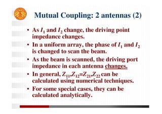
14. Fourier Transform Method :
Linear Array
14
For an odd number of elements, the array factor is given by





M
M
m
jm
me
a 

 )
(
)
( AF
AF
where
For an even number of elements,
















1
2
1
2
1
2
1
2
'
m
M
d
m
M
m
d
m
zm
M
m
md
zm 



 ,
,
2
,
1
,
0
,
'
K
Elements’ locations

 








M
m
m
j
m
M
m
m
j
m e
a
e
a
1
]
2
/
)
1
2
[(
1
]
2
/
)
1
2
[(
)
(
)
( 


 AF
AF


 
 cos
kd
Even-number
Odd-number

15. Fourier Transform Method :
Linear Array (2)
15
For an odd number of elements, the excitation coefficients can
be obtained by
M
m
M
d
e
d
e
T
a jm
jm
T
T
m




 


 
 



 



)
(
2
1
)
(
1 2
/
2
/
AF
AF
where
For an even number of elements,


 
 cos
kd




















M
m
d
e
m
M
d
e
a
m
j
m
j
m
1
)
(
2
1
1
)
(
2
1
]
2
/
)
1
2
[(
]
2
/
)
1
2
[(












AF
AF

16. Fourier Transform Method :
Example
16
Same as Example 7.2 with d = λ/2; non-zero only
2
/
cos
2
/ 



 



 kd
4
/
3
4
/ 

 

thus
therefore
2
2
sin
2
1
2
1 2
/
2
/ 






m
m
d
e
a jm
m







 

0101
.
0
0588
.
0
010
.
0
0518
.
0
2170
.
0
0455
.
0
0895
.
0
3582
.
0
0496
.
0
0578
.
0
0
.
1
7
3
10
6
2
9
5
1
8
4
0

























a
a
a
a
a
a
a
a
a
a
a
Result

17. Fourier Transform Method :
Example

18. Quiz
A 5-element uniform linear array with a
spacing of λ
λ
λ
λ between elements is designed
to scan at θ
θ
θ
θ=π
π
π
π/3. Assume that the array is
aligned along the z-axis.
a) Find the array factor
b) Find the angle of the grating lobe.
c) Find the condition such that there exists no
grating lobe.

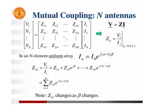
19. Quiz solution
0 20 40 60 80 100 120 140 160 180
0
0.1
0.2
0.3
0.4
0.5
0.6
0.7
0.8
0.9
1
θ [Degree]
|(AF)
n
|
[dB]
5−element array factor
d=λ
d=5λ/8
d=λ/2

20. Woodward-Lawson Method
• Sampling the desired pattern at various discrete
locations.
• Use composing function of the forms:
as the field of each pattern sample
• The synthesized pattern is represented by a finite
sum of composing functions.
• The total excitation is a sum of space harmonics.
m
m
m
m
m
m N
N
b
b 


 sin
/
)
sin(
or
/
)
sin(

21. Woodward-Lawson Method:
Line-source
2
/
'
2
/
)
'
( cos
'
l
z
l
e
l
b
z
i m
jkz
m
m 


  





M
M
m
jkz
m
m
e
b
l
z
I 
cos
'
1
)
'
(
number)
odd
1
2
(for
,
,
2
,
1
,
0
number)
even
2
(for
,
,
2
,
1
where









M
M
m
M
M
m
K
K
 
 
m
m
m
m
kl
kl
b
s





cos
cos
2
cos
cos
2
sin
)
(









Let the source be represented by a sum of the following constant
current source of length l.
Then the current source can be given by
The field pattern of each current source is given by
Composing function

22. Woodward-Lawson Method:
Line-source (2)
d
m
m
b )
(
SF 
 

l
kz l
z

 



  2
' '|
|
For an odd number samples, the total pattern becomes
bm can be obtained from the value at the sample points θm, i.e.,
In order to satisfy the periodicity of 2π and faithfully reconstruct
the desired pattern,
 
 












M
M
m
m
m
m
kl
kl
b





cos
cos
2
cos
cos
2
sin
)
(
SF

23. Woodward-Lawson Method:
Line-source (3)
samples
odd
for
,
2
,
1
,
0
,
cos K











 m
l
m
m
m


Thus the location of each sample is given by
Therefore, M should be the closest integer to M=l/λ.
samples
even
for
,
2
,
1
,
2
1
2
2
1
2
,
2
,
1
,
2
1
2
2
1
2
cos
































K
K
m
l
m
m
m
l
m
m
m




24. Woodward-Lawson Method:
Example
5
,
,
2
,
1
,
0
),
2
.
0
(
cos
)
(
cos 1
1






 

K
m
m
m
m

Same as Example 7.2; for l = 5λ.
Since l = 5λ, M = 5 and ∆ = 0.2.
m θ
θ
θ
θm bm
m θ
θ
θ
θm bm
0 90 1
1 78.46 1 -1 101.54 1
2 66.42 1 -2 113.58 1
3 53.13 1 -3 126.87 1
4 36.87 0 -4 143.13 0
5 0 0 -5 180 0

25. Woodward-Lawson Method:
Example (2)
Composing functions for line-source (l = 5λ)

26. Woodward-Lawson Method:
Linear array
 
 
m
m
m
m
kd
N
kd
N
b
f





cos
cos
2
sin
cos
cos
2
sin
)
(









The pattern of each sample (uniform array) can be written as
(assuming l = Nd)
Composing function
 
 












M
M
m
m
m
m
kd
N
kd
N
b





cos
cos
2
sin
cos
cos
2
sin
)
(
AF
d
m
m
b )
(
AF 
 

For an odd number elements, the array factor becomes
bm can be obtained from the value at the sample points θm, i.e.,

27. Woodward-Lawson Method:
Linear array (2)
samples
even
for
,
2
,
1
,
2
1
2
2
1
2
,
2
,
1
,
2
1
2
2
1
2
cos
































K
K
m
Nd
m
m
m
Nd
m
m
m



samples
odd
for
,
2
,
1
,
0
,
cos K











 m
Nd
m
m
m


The location of each sample is given by
The normalized excitation coefficient of each element is given by






M
M
m
z
jk
m
n
m
n
e
b
N
z
a 
cos
1
)
'
(

28. Woodward-Lawson Method:
Example
Element number
n
Position
z’n
Coefficient
an
±1 ±0.25λ
λ
λ
λ 0.5696
±2 ± 0.75λ
λ
λ
λ -0.0345
±3 ± 1.25λ
λ
λ
λ -0.1001
±4 ± 1.75λ
λ
λ
λ 0.1108
±5 ± 2.25λ
λ
λ
λ -0.0460
Same as Example 7.2; for N=10 and d = λ/2.
The coefficients can be found to be
To obtain the normalized amplitude pattern of unity at θ=π/2,
the array factor has been divided by   4998
.
0
n
a

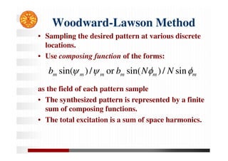
29. Woodward-Lawson Method:
Example
0 20 40 60 80 100 120 140 160 180
0
0.2
0.4
0.6
0.8
1
1.2
1.4
θ [Degree]
Normalized
magnitude
Line−source
Linear Array (N=10,d=λ/2)

30. Triangular, cosine, cosine
squared distributions

32. 32
Mutual Coupling
• Consider two antennas
2
22
1
21
2
2
12
1
11
1
I
Z
I
Z
V
I
Z
I
Z
V























2
1
22
21
12
11
2
1
I
I
Z
Z
Z
Z
V
V
21
12 Z
Z 
If reciprocal,
Equivalent Circuit
Two-port Network
T-Network Equivalent Circuit

33. Mutual Coupling: 2 antennas
0
1
1
11
2 

I
I
V
Z
0
2
1
12
1 

I
I
V
Z
0
1
2
21
2 

I
I
V
Z
0
2
2
22
1 

I
I
V
Z
impedance
point
driving
active
2
1




d
d
Z
1
2
12
11
1
1
1
I
I
Z
Z
I
V
Z d 


21
12 Z
Z 
for reciprocal networks
:
, 22
11 Z
Z
Input impedance
2
1
21
22
2
2
2
I
I
Z
Z
I
V
Z d 


2
1
2
1
2
1 on
depends
;
on
depends
:
Note
I
I
Z
I
I
Z d
d

34. Mutual Coupling: 2 antennas (2)
• As I1 and I2 change, the driving point
impedance changes.
• In a uniform array, the phase of I1 and I2
is changed to scan the beam.
• As the beam is scanned, the driving port
impedance in each antenna changes.
• In general, Z11,Z12=Z21,Z22 can be
calculated using numerical techniques.
• For some special cases, they can be
calculated analytically.

35. Mutual Coupling: N antennas





































N
NN
N
N
N
N
N I
I
I
Z
Z
Z
Z
Z
Z
Z
Z
Z
V
V
V
M
L
M
O
M
M
L
L
M
2
1
2
1
2
22
21
1
12
11
2
1 I
Z
V 
j
k
I
j
i
ij
k
I
V
Z



,
0
In an N-element uniform array 
)
1
(
0

 n
j
n e
I
I










N
n
n
j
n
N
j
N
j
d
e
Z
e
Z
e
Z
Z
I
V
Z
1
)
1
(
1
)
1
(
1
12
11
1
1
1



L
changes.
as
changes
:
Note 1 
d
Z

36. Mutual Coupling: 2 dipoles

37. Mutual Coupling: 2 dipoles (2)