
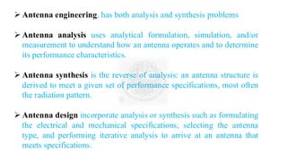
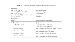
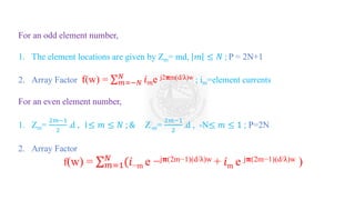
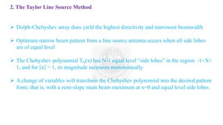
![2. Woodward–Lawson Sampling Method
➢ This method is analogous to Woodward–Lawson sampling method for line sources
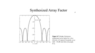
➢ The synthesized array factor is the superposition of array factors from uniform
amplitude, linear phase arrays
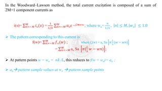
➢ f(w)=σ𝑛=−𝑀
𝑀
𝑎𝑛
sin[
𝑝
2
𝑤−𝑤𝑛
2𝛑
λ
𝑑]
P sin[
1
2
𝑤−𝑤𝑛
2𝛑
λ
𝑑]
➢ where the sample values are an= fd(w=wn); & wn= n (
λ
𝑃𝑑
) =
𝑛
𝑙/λ
, 𝑛 ≤ 𝑀, 𝑤𝑛 ≤1.0
➢ The element currents required to give this pattern are
im =(1/p) σ𝑛=−𝑀
𝑀
𝑎𝑛e −j2𝛑(Zm/λ)wn → for either even or odd elements](https://image.slidesharecdn.com/ch2module2antennasynthesis-250113111118-fb1d55e0/85/CH2-Antenna-Theory-and-Design-Course-Code-22LDN22-for-M-Tech-VTU-20-320.jpg)
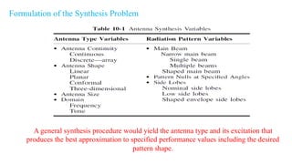
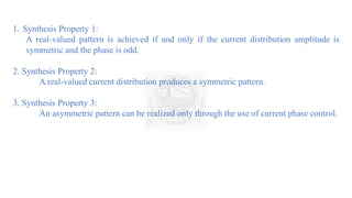
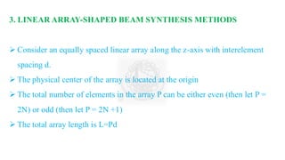
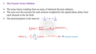
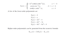
![3. Comparison of Shaped Beam Synthesis Method
➢ Three distinct types of pattern regions: side lobe, main beam, and transition
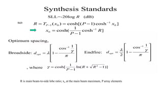
➢ Over the side lobe region, SLL is defined as
SLL= 20 log
𝑣𝑎𝑙𝑢𝑒 𝑜𝑓 𝑡ℎ𝑒 ℎ𝑖𝑔ℎ𝑒𝑠𝑡 𝑠𝑖𝑑𝑒 𝑙𝑜𝑏𝑒 𝑝𝑒𝑎𝑘
max 𝑜𝑓 𝑑𝑒𝑠𝑖𝑟𝑒𝑑 𝑝𝑎𝑡𝑡𝑒𝑟𝑚
➢ Over the main lobe region the measure of Ripple R is
R = 20 max log
𝑓(𝑤)
𝑓𝑑(𝑤)
[db]
➢ The Transition width T, which gives a measure of fall of main beam in side
lobe region is T = 𝑤𝑓 = 0.9 −
𝑤𝑓 = 0.1 ;
➢ 𝑤𝑓=0.9 & 𝑤𝑓=0.1 are discontinuity in the desired pattern at w=90 & 10 %
The shaped beam synthesis methods can be compared easily using
SLL, R, and T.
➢ The Woodward–
Lawson methods
produce low side
lobes and low
main beam
ripple at some
sacrifice in
transition width.
➢ Fourier methods
yield somewhat
inferior side lobe
levels, ripples
&small
transition width](https://image.slidesharecdn.com/ch2module2antennasynthesis-250113111118-fb1d55e0/85/CH2-Antenna-Theory-and-Design-Course-Code-22LDN22-for-M-Tech-VTU-22-320.jpg)


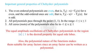
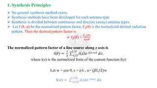
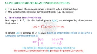
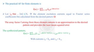
![Symmetrically Excited, Broadside Array
➢ i-m= im ; zm=md, &
➢ i0 is at origin (z = 0), ψ= 2𝜋(d/λ)𝑤
➢ f(ψ) = ቐ
𝑖0 + 2 σ𝑚=1
𝑁
𝑖𝑚𝑐𝑜𝑠𝑚ψ 𝑃 𝑜𝑑𝑑
2 σ𝑚=1
𝑁
𝑖𝑚𝑐𝑜𝑠[
2𝑚−1 ψ
2
]
P even
➢ Using trigonometric identities, cos(mψ) = σ𝑚=1
𝑁
𝑐𝑜𝑠[
ψ
2
])
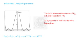
➢ Let x= x0cos ψ/2 then f(ψ) = Tp-1(x0cos ψ/2 ) ;
➢ 𝜃 = 900 → a broadside array.
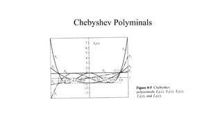
Chebyshev polynomial T4(x)](https://image.slidesharecdn.com/ch2module2antennasynthesis-250113111118-fb1d55e0/85/CH2-Antenna-Theory-and-Design-Course-Code-22LDN22-for-M-Tech-VTU-30-320.jpg)

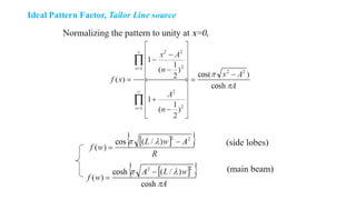
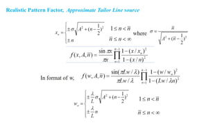
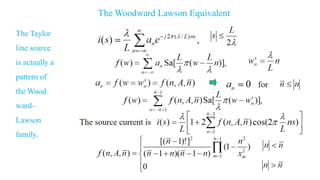
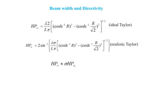

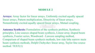
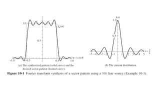
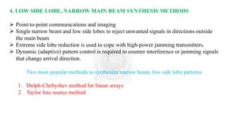
The document discusses antenna synthesis principles and methods, focusing on factors influencing linear arrays and radiation patterns. It outlines mathematical formulations and sampling techniques for synthesizing desired patterns, including methods such as the Woodward–Lawson method and Dolph-Chebyshev approach. The methods aim to optimize antenna performance, notably in achieving low side lobes and narrow main beams for applications in communications and imaging.


![3_Antenna Array [Modlue 4] (1).pdf](https://cdn.slidesharecdn.com/ss_thumbnails/3antennaarraymodlue41-220419112111-thumbnail.jpg?width=640&height=640&fit=bounds)