The document contains multiple articles featured in the January 2014 issue of the International Journal of Computer Science and Business Informatics, focusing on diverse topics including stock data analysis using SVM-PCA, mobile malware, UML inconsistencies, portfolio optimization, and emerging technologies. It highlights a case study on predicting stock prices using support vector machines and principal component analysis, demonstrating the model's effectiveness in improving prediction accuracy. The articles are contributions from various authors in the fields of computer science and engineering.


![International Journal of Computer Science and Business Informatics
IJCSBI.ORG
ISSN: 1694-2108 | Vol. 9, No. 1. JANUARY 2014 1
A Predictive Stock Data Analysis
with SVM-PCA Model
Divya Joseph
PG Scholar, Department of Computer Science and Engineering
Christ University Faculty of Engineering
Christ University, Kanmanike, Mysore Road, Bangalore - 560060
Vinai George Biju
Asst. Professor, Department of Computer Science and Engineering
Christ University Faculty of Engineering
Christ University, Kanmanike, Mysore Road, Bangalore – 560060
ABSTRACT
In this paper the properties of Support Vector Machines (SVM) on the financial time series
data has been analyzed. The high dimensional stock data consists of many features or
attributes. Most of the attributes of features are uninformative for classification. Detecting
trends of stock market data is a difficult task as they have complex, nonlinear, dynamic and
chaotic behaviour. To improve the forecasting of stock data performance different models
can be combined to increase the capture of different data patterns. The performance of the
model can be improved by using only the informative attributes for prediction. The
uninformative attributes are removed to increase the efficiency of the model. The
uninformative attributes from the stock data are eliminated using the dimensionality
reduction technique: Principal Component Analysis (PCA). The classification accuracy of
the stock data is compared when all the attributes of stock data are being considered that is,
SVM without PCA and the SVM-PCA model which consists of informative attributes.
Keywords
Machine Learning, stock analysis, prediction, support vector machines, principal
component analysis.
1. INTRODUCTION
Time series analysis and prediction is an important task in all fields of
science for applications like forecasting the weather, forecasting the
electricity demand, research in medical sciences, financial forecasting,
process monitoring and process control, etc [1][2][3]. Machine learning
techniques are widely used for solving pattern prediction problems. The
financial time series stock prediction is considered to be a very challenging
task for analysts, investigator and economists [4]. A vast number of studies
in the past have used artificial neural networks (ANN) and genetic
algorithms for the time series data [5]. Many real time applications are using
the ANN tool for time-series modelling and forecasting [6]. Furthermore the](https://image.slidesharecdn.com/vol9no1-january2014-171208072155/85/Vol-9-No-1-January-2014-4-320.jpg)
![International Journal of Computer Science and Business Informatics
IJCSBI.ORG
ISSN: 1694-2108 | Vol. 9, No. 1. JANUARY 2014 2
researchers hybridized the artificial intelligence techniques. Kohara et al. [7]
incorporated prior knowledge to improve the performance of stock market
prediction. Tsaih et al. [8] integrated the rule-based technique and ANN to
predict the direction of the S& P 500 stock index futures on a daily basis.
Some of these studies, however, showed that ANN had some limitations in
learning the patterns because stock market data has tremendous noise and
complex dimensionality [9]. ANN often exhibits inconsistent and
unpredictable performance on noisy data [10]. However, back-propagation
(BP) neural network, the most popular neural network model, suffers from
difficulty in selecting a large number of controlling parameters which
include relevant input variables, hidden layer size, learning rate, and
momentum term [11].
This paper proceeds as follows. In the next section, the concepts of support
vector machines. Section 3 describes the principal component analysis.
Section 4 describes the implementation and model used for the prediction of
stock price index. Section 5 provides the results of the models. Section 6
presents the conclusion.
2. SUPPORT VECTOR MACHINES
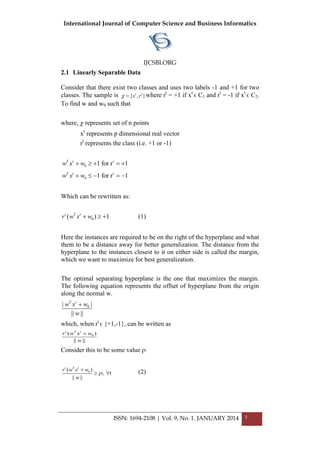
Support vector machines (SVMs) are very popular linear discrimination
methods that build on a simple yet powerful idea [12]. Samples are mapped
from the original input space into a high-dimensional feature space, in
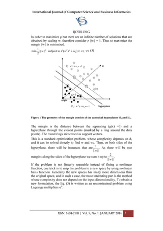
which a „best‟ separating hyperplane can be found. A separating hyperplane
H is best if its margin is largest [13].
The margin is defined as the largest distance between two hyperplanes
parallel to H on both sides that do not contain sample points between them
(we will see later a refinement to this definition) [12]. It follows from the
risk minimization principle (an assessment of the expected loss or error, i.e.,
the misclassification of samples) that the generalization error of the
classifier is better if the margin is larger.
The separating hyperplane that are the closest points for different classes at
maximum distance from it is preferred, as the two groups of samples are
separated from each other by a largest margin, and thus least sensitive to
minor errors in the hyperplane‟s direction [14].](https://image.slidesharecdn.com/vol9no1-january2014-171208072155/85/Vol-9-No-1-January-2014-5-320.jpg)
![International Journal of Computer Science and Business Informatics
IJCSBI.ORG
ISSN: 1694-2108 | Vol. 9, No. 1. JANUARY 2014 5
2
0
1
2
0
1 1
1
|| || [ ( ) 1]
2
1
= || || ( ) +
2
N
t t T t
p
t
t t T t t
t t
L w r w x w
w r w x w
This can be minimized with respect to w, w0 and maximized with respect to
αt
≥ 0. The saddle point gives the solution.
This is a convex quadratic optimization problem because the main term is
convex and the linear constraints are also convex. Therefore, the dual
problem is solved equivalently by making use of the Karush-Kuhn-Tucker
conditions. The dual is to maximize Lp with respect to w and w0 are 0 and
also that αt
≥ 0.
1
0 w =
n
p t t t
i
L
r x
w
(5)
10
0 w = = 0
n
p t t
i
L
r
w
(6)
Substituting Eq. (5) and Eq. (6) in Eq. (4), the following is obtained:
0
1
( )
2
T T t t t t t t
d
t t t
L w w w r x w r
1
= - ( )
2
t s t s t T s t
t s t
r x x x (7)
which can be minimized with respect to αt
only, subject to the constraints
0, and 0, tt t t
t
r
This can be solved using the quadratic optimization methods. The size of the
dual depends on N, sample size, and not on d, the input dimensionality.](https://image.slidesharecdn.com/vol9no1-january2014-171208072155/85/Vol-9-No-1-January-2014-8-320.jpg)
![International Journal of Computer Science and Business Informatics
IJCSBI.ORG
ISSN: 1694-2108 | Vol. 9, No. 1. JANUARY 2014 6
Once αt
is solved only a small percentage have αt
> 0 as most of them vanish
with αt
= 0.
The set of xt
whose xt
> 0 are the support vectors, then w is written as
weighted sum of these training instances that are selected as support vectors.
These are the xt
that satisfy and lie on the margin. This can be used to
calculate w0 from any support vector as
0
t T t
w r w x (8)
For numerical stability it is advised that this be done for all support vectors
and average be taken. The discriminant thus found is called support vector
machine (SVM) [1].
3. PRINCIPAL COMPONENT ANALYSIS
Principal Component Analysis (PCA) is a powerful tool for dimensionality
reduction. The advantage of PCA is that if the data patterns are understood
then the data is compressed by reducing the number of dimensions. The
information loss is considerably less.
Figure 2 Diagrammatic Representation of Principal Component Analysis (PCA)](https://image.slidesharecdn.com/vol9no1-january2014-171208072155/85/Vol-9-No-1-January-2014-9-320.jpg)
![International Journal of Computer Science and Business Informatics
IJCSBI.ORG
ISSN: 1694-2108 | Vol. 9, No. 1. JANUARY 2014 8
training data [15]. The cross validation variable k is set to 10 for the stock
dataset [16].The cross-validation process is then repeated k times (the folds),
with each of the k subsamples used exactly once as the validation data. The
k results from the folds then can be averaged (or otherwise combined) to
produce a single estimation.
Figure 3 Weka Screenshot of PCA
At first the model is trained with SVM and the results with the test data is
saved. Second, the dimensionality reduction technique such as PCA is
applied to the training dataset. The PCA selects the attributes which give
more information for the stock index classification. The number of attributes
for classification is now reduced from 30 attributes to 5 attributes.
The most informative attributes are only being considered for classification.
A new model is trained on SVM with the reduced attributes. The test data
with reduces attributes is provided to the model and the result is saved. The
results of both the models are compared and analysed.
5. EXPERIMENTAL RESULTS
5.1 Classification without using PCA
From the tables displayed below 300 stock index instances were considered
as training data and 100 stock index instances were considered as test data.
With respect to the test data 43% instances were correctly classified and
57% instances were incorrectly classified.](https://image.slidesharecdn.com/vol9no1-january2014-171208072155/85/Vol-9-No-1-January-2014-11-320.jpg)
![International Journal of Computer Science and Business Informatics
IJCSBI.ORG
ISSN: 1694-2108 | Vol. 9, No. 1. JANUARY 2014 10
features. In this way a better idea about the stock data is obtained and in turn
gives an efficient knowledge extraction on the stock indices. The stock data
classified better with SVM-PCA model when compared to the classification
with SVM alone. The SVM-PCA model also reduces the computational cost
drastically. The instances are labelled with nominal values for the current
case study. The future enhancement to this paper would be to use numerical
values for labelling instead of nominal values.
7. ACKNOWLEDGMENTS
We express our sincere gratitude to the Computer Science and Engineering
Department of Christ University Faculty of Engineering especially
Prof. K Balachandran for his constant motivation and support.
REFERENCES
[1] Divya Joseph, Vinai George Biju, “A Review of Classifying High Dimensional Data to
Small Subspaces”, Proceedings of International Conference on Business Intelligence at
IIM Bangalore, 2013.
[2] Claudio V. Ribeiro, Ronaldo R. Goldschmidt, Ricardo Choren, A Reuse-based
Environment to Build Ensembles for Time Series Forecasting, Journal of Software,
Vol. 7, No. 11, Pages 2450-2459, 2012.
[3] Dr. A. Chitra, S. Uma, "An Ensemble Model of Multiple Classifiers for Time Series
Prediction", International Journal of Computer Theory and Engineering, Vol. 2, No. 3,
pages 454-458, 2010.
[4] Sundaresh Ramnath, Steve Rock, Philip Shane, "The financial analyst forecasting
literature: A taxonomy with suggestions for further research", International Journal of
Forecasting 24 (2008) 34–75.
[5] Konstantinos Theofilatos, Spiros Likothanassis, Andreas Karathanasopoulos, Modeling
and Trading the EUR/USD Exchange Rate Using Machine Learning Techniques,
ETASR - Engineering, Technology & Applied Science Research Vol. 2, No. 5, pages
269-272, 2012.
[6] A simulation study of artificial neural networks for nonlinear time-series forecasting.
G. Peter Zhang, B. Eddy Patuwo, and Michael Y. Hu. Computers & OR 28(4):381-
396 (2001)
[7] K. Kohara, T. Ishikawa, Y. Fukuhara, Y. Nakamura, Stock price prediction using prior
knowledge and neural networks, Int. J. Intell. Syst. Accounting Finance Manage. 6 (1)
(1997) 11–22.
[8] R. Tsaih, Y. Hsu, C.C. Lai, Forecasting S& P 500 stock index futures with a hybrid AI
system, Decision Support Syst. 23 (2) (1998) 161–174.
[9] Mahesh Khadka, K. M. George, Nohpill Park, "Performance Analysis of Hybrid
Forecasting Model In Stock Market Forecasting", International Journal of Managing
Information Technology (IJMIT), Vol. 4, No. 3, August 2012.
[10]Kyoung-jae Kim, “Artificial neural networks with evolutionary instance selection for
financial forecasting. Expert System. Application 30, 3 (April 2006), 519-526.
[11]Guoqiang Zhang, B. Eddy Patuwo, Michael Y. Hu, “Forecasting with artificial neural
networks: The state of the art”, International Journal of Forecasting 14 (1998) 35–62.](https://image.slidesharecdn.com/vol9no1-january2014-171208072155/85/Vol-9-No-1-January-2014-13-320.jpg)
![International Journal of Computer Science and Business Informatics
IJCSBI.ORG
ISSN: 1694-2108 | Vol. 9, No. 1. JANUARY 2014 11
[12]K. Kim, I. Han, Genetic algorithms approach to feature discretization in artificial
neural networks for the prediction of stock price index, Expert Syst. Appl. 19 (2)
(2000) 125–132.
[13]F. Cai and V. Cherkassky “Generalized SMO algorithm for SVM-based multitask
learning", IEEE Trans. Neural Netw. Learn. Syst., Vol. 23, No. 6, pp.997 -1003, 2012.
[14]Corinna Cortes and Vladimir Vapnik, Support-Vector Networks. Mach. Learn. 20,
Volume 3, 273-297, 1995.
[15]Shivanee Pandey, Rohit Miri, S. R. Tandan, "Diagnosis And Classification Of
Hypothyroid Disease Using Data Mining Techniques", International Journal of
Engineering Research & Technology, Volume 2 - Issue 6, June 2013.
[16]Hui Shen, William J. Welch and Jacqueline M. Hughes-Oliver, "Efficient, Adaptive
Cross-Validation for Tuning and Comparing Models, with Application to Drug
Discovery", The Annals of Applied Statistics 2011, Vol. 5, No. 4, 2668–2687,
February 2012, Institute of Mathematical Statistics.
This paper may be cited as:
Joseph, D. and Biju, V. G., 2014. A Predictive Stock Data Analysis with
SVM-PCA Model. International Journal of Computer Science and Business
Informatics, Vol. 9, No. 1, pp. 1-11.](https://image.slidesharecdn.com/vol9no1-january2014-171208072155/85/Vol-9-No-1-January-2014-14-320.jpg)
![International Journal of Computer Science and Business Informatics
IJCSBI.ORG
ISSN: 1694-2108 | Vol. 9, No. 1. JANUARY 2014 12
HOV-kNN: A New Algorithm to
Nearest Neighbor Search in
Dynamic Space
Mohammad Reza Abbasifard
Department of Computer Engineering,
Iran University of Science and Technology,
Tehran, Iran
Hassan Naderi
Department of Computer Engineering,
Iran University of Science and Technology,
Tehran, Iran
Mohadese Mirjalili
Department of Computer Engineering,
Iran University of Science and Technology,
Tehran, Iran
ABSTRACT
Nearest neighbor search is one of the most important problem in computer science due to
its numerous applications. Recently, researchers have difficulty to find nearest neighbors in
a dynamic space. Unfortunately, in contrast to static space, there are not many works in this
new area. In this paper we introduce a new nearest neighbor search algorithm (called
HOV-kNN) suitable for dynamic space due to eliminating widespread preprocessing step in
static approaches. The basic idea of our algorithm is eliminating unnecessary computations
in Higher Order Voronoi Diagram (HOVD) to efficiently find nearest neighbors. The
proposed algorithm can report k-nearest neighbor with time complexity O(knlogn) in
contrast to previous work which wasO(k2
nlogn). In order to show its accuracy, we have
implemented this algorithm and evaluated is using an automatic and randomly generated
data point set.
Keywords
Nearest Neighbor search, Dynamic Space, Higher Order Voronoi Diagram.
1. INTRODUCTION
The Nearest Neighbor search (NNS) is one of the main problems in
computer science with numerous applications such as: pattern recognition,
machine learning, information retrieval and spatio-temporal databases [1-6].
Different approaches and algorithms have been proposed to these diverse
applications. In a well-known categorization, these approaches and
algorithms could be divided into static and dynamic (moving points). The](https://image.slidesharecdn.com/vol9no1-january2014-171208072155/85/Vol-9-No-1-January-2014-15-320.jpg)
![International Journal of Computer Science and Business Informatics
IJCSBI.ORG
ISSN: 1694-2108 | Vol. 9, No. 1. JANUARY 2014 13
existing algorithms and approaches can be divided into three categories,
based on the fact that whether the query points and/or data objects are
moving. They are (i) static kNN query for static objects, (ii) moving
kNNquery for static objects, and (iii) moving kNN query for moving objects
[15].
In the first category data points as well as query point(s) have stationary
positions [4, 5]. Most of these approaches, first index data points by
performing a pre-processing operation in order to constructing a specific
data structure. It’s usually possible to carry out different search algorithms
on a given data structure to find nearest neighbors. Unfortunately, the pre-
processing step, index construction, has a high complexity and takes more
time in comparison to search step. This time could be reasonable when the
space is static, because by just constructing the data structure multiple
queries can be accomplished. In other words, taken time to pre-processing
step will be amortized over query execution time. In this case, searching
algorithm has a logarithmic time complexity. Therefore, these approaches
are useful, when it’s necessary to have a high velocity query execution on
large stationary data volume.
Some applications need to have the answer to a query as soon as the data is
accessible, and they cannot tolerate the pre-processing execution time. For
example, in a dynamic space when data points are moving, spending such
time to construct a temporary index is illogical. As a result approaches that
act very well in static space may be useless in dynamic one.
In this paper a new method, so called HOV-kNN, suitable for finding k
nearest neighbor in a dynamic environment, will be presented. In k-nearest
neighbor search problem, given a set P of points in a d-dimensional
Euclidian space𝑅 𝑑
(𝑃 ⊂ 𝑅 𝑑
) and a query point q (𝑞 ∈ 𝑅 𝑑
), the problem is
to find k nearest points to the given query point q [2, 7]. Proposed algorithm
has a good query execution complexity 𝑂(𝑘𝑛𝑙𝑜𝑔𝑛) without enduring from
time-consuming pre-processing process. This approach is based on the well-
known Voronoi diagrams (VD) [11]. As an innovation, we have changed the
Fortune algorithm [13] in order to created order k Voronoi diagrams that
will be used for finding kNN.
The organization of this paper is as follow. Next section gives an overview
on related works. In section 3 basic concepts and definitions have been
presented. Section 4 our new approach HOV-kNN is explained. Our
experimental results are discussed in section 5. We have finished our paper
with a conclusion and future woks in section 6.
2. RELATED WORKS
Recently, many methods have been proposed for k-nearest neighbor search
problem. A naive solution for the NNS problem is using linear search](https://image.slidesharecdn.com/vol9no1-january2014-171208072155/85/Vol-9-No-1-January-2014-16-320.jpg)
![International Journal of Computer Science and Business Informatics
IJCSBI.ORG
ISSN: 1694-2108 | Vol. 9, No. 1. JANUARY 2014 14
method that computes distance from the query to every single point in the
dataset and returns the k closest points. This approach is guaranteed to find
the exact nearest neighbors [6]. However, this solution can be expensive for
massive datasets. So approximate nearest neighbor search algorithms are
presented even for static spaces [2].
One of the main parts in NNS problem is data structure that is roughly used
in every approach. Among different data structures, various tree search most
used structures which can be applied in both static and dynamic spaces.
Listing proposed solutions to kNN for static space is out of scope of this
paper. The interested reader can refer to more comprehensive and detailed
discussions of this subject by [4, 5]. Just to name some more important
structures, we can point to kd-tree, ball-tree, R-tree, R*-tree, B-tree and X-
tree [2-5, 8, 9].In contrast, there are a number of papers that use graph data
structure for nearest neighbor search. For example, Hajebi et al have
performed Hill-climbing in kNN graph. They built a nearest neighbor graph
in an offline phase, and performed a greedy search on it to find the closest
node to the query [6].
However, the focus of this paper is on dynamic space. In contrast to static
space, finding nearest neighbors in a dynamic environment is a new topic of
research with relatively limited number of publications. Song and
Roussopoulos have proposed Fixed Upper Bound Algorithm, Lazy Search
Algorithm, Pre-fetching Search Algorithm and Dual Buffer Search to find k-
nearest neighbors for a moving query point in a static space with stationary
data points [8]. Güting et al have presented a filter-and-refine approach to
kNN search problem in a space that both data points and query points are
moving. The filter step traverses the index and creates a stream of so-called
units (linear pieces of a trajectory) as a superset of the units required to build
query’s results. The refinement step processes an ordered stream of units
and determines the pieces of units forming the final precise result
[9].Frentzos et al showed mechanisms to perform NN search on structures
such as R-tree, TB-Tree, 3D-R-Tree for moving objects trajectories. They
used depth-first and best-first algorithms in their method [10].
As mentioned, we use Voronoi diagram [11] to find kNN in a dynamic
space. D.T. Lee used Voronoi diagram to find k nearest neighbor. He
described an algorithm for computing order-k Voronoi diagram in
𝑂(𝑘2
𝑛𝑙𝑜𝑔𝑛) time and 𝑂(𝑘2
(𝑁 − 𝑘)) space [12] which is a sequential
algorithm. Henning Meyerhenke presented and analyzed a parallel
algorithm for constructing HOVD for two parallel models: PRAM and CGM
[14]. In these models he used Lee’s iterative approach but his model stake
𝑂
𝑘2(𝑛−𝑘)𝑙𝑜𝑔𝑛
𝑝
running time and 𝑂(𝑘) communication rounds on a CGM](https://image.slidesharecdn.com/vol9no1-january2014-171208072155/85/Vol-9-No-1-January-2014-17-320.jpg)
![International Journal of Computer Science and Business Informatics
IJCSBI.ORG
ISSN: 1694-2108 | Vol. 9, No. 1. JANUARY 2014 15
with 𝑂(
𝑘2(𝑁−𝑘)
𝑝
) local memory per processor [14]. p is the number of
participant machines.
3. BASIC CONCEPTS AND DEFINITIONS
Let P be a set of n sites (points) in the Euclidean plane. The Voronoi
diagram informally is a subdivision of the plane into cells (Figure 1)which
each point of that has the same closest site [11].
Figure 1.Voronoi Diagram
Euclidean distance between two points p and q is denoted by 𝑑𝑖𝑠𝑡 𝑝, 𝑞 :
𝑑𝑖𝑠𝑡 𝑝, 𝑞 : = (𝑝𝑥 − 𝑞𝑥)2 + (𝑝𝑦 − 𝑞𝑦)2 (1)
Definition (Voronoi diagram):Let 𝑃 = {𝑝1, 𝑝2, … , 𝑝 𝑛 } be a set of n distinct
points (so called sites) in the plane. Voronoi diagram of P is defined as the
subdivision of the plane into n cells, one for each site in P, with the
characteristic that q in the cell corresponding to site 𝑝𝑖 if𝑑𝑖𝑠𝑡 𝑞, 𝑝𝑖 <
𝑑𝑖𝑠𝑡 𝑞, 𝑝𝑗 for each 𝑝𝑗 ∈ 𝑃 𝑤𝑖𝑡ℎ 𝑗 ≠ 𝑖 [11].
Historically, 𝑂(𝑛2
)incremental algorithms for computing VD were known
for many years. Then 𝑂 𝑛𝑙𝑜𝑔𝑛 algorithm was introduced that this
algorithm was based on divide and conquer, which was complex and
difficult to understand. Then Steven Fortune [13] proposed a plane sweep
algorithm, which provided a simpler 𝑂 𝑛𝑙𝑜𝑔𝑛 solution to the problem.
Instead of partitioning the space into regions according to the closest sites,
one can also partition it according to the k closest sites, for some 1 ≤ 𝑘 ≤
𝑛 − 1. The diagrams obtained in this way are called higher-order Voronoi
diagrams or HOVD, and for given k, the diagram is called the order-k
Voronoi diagram [11]. Note that the order-1 Voronoi diagram is nothing
more than the standard VD. The order-(n−1) Voronoi diagram is the
farthest-point Voronoi diagram (Given a set P of points in the plane, a point
of P has a cell in the farthest-point VD if it is a vertex of the convex hull),
because the Voronoi cell of a point 𝑝𝑖 is now the region of points for which
𝑝𝑖 is the farthest site. Currently the best known algorithms for computing the](https://image.slidesharecdn.com/vol9no1-january2014-171208072155/85/Vol-9-No-1-January-2014-18-320.jpg)
![International Journal of Computer Science and Business Informatics
IJCSBI.ORG
ISSN: 1694-2108 | Vol. 9, No. 1. JANUARY 2014 16
order-k Voronoi diagram run in 𝑂(𝑛𝑙𝑜𝑔3
𝑛 + 𝑛𝑘) time and in 𝑂(𝑛𝑙𝑜𝑔𝑛 +
𝑛𝑘2 𝑐𝑙𝑜𝑔 ∗ 𝑘
) time, where c is a constant [11].
Figure 2. Farthest-Point Voronoi diagram [11]
Consider x and y as two distinct elements of P. A set of points construct a
cell in the second order Voronoi diagram for which the nearest and the
second nearest neighbors are x and y. Second order Voronoi diagram can be
used when we are interested in the two closest points, and we want a
diagram to captures that.
Figure 3.An instant of HOVD [11]
4. SUGGESTED ALGORITHM
As mentioned before, one of the best algorithms to construct Voronoi
diagram is Fortune algorithm. Furthermore HOVD can be used to find k-
nearest neighbors [12]. D.T. Lee used an 𝑂 𝑘2
𝑛𝑙𝑜𝑔𝑛 algorithm to
construct a complete HOVD to obtain nearest neighbors. In D.T. Lee's
algorithm, at first the first order Voronoi diagram is obtained, and then finds
the region of diagram that contains query point. The point that is in this
region is defined as a first neighbor of query point. In the next step of Lee’s
algorithm, this nearest point to the query will be omitted from dataset, and
this process will be repeated. In other words, the Voronoi diagram is built
on the rest of points. In the second repetition of this process, the second
neighbor is found and so on. So the nearer neighbors to a given query point
are found sequentially.](https://image.slidesharecdn.com/vol9no1-january2014-171208072155/85/Vol-9-No-1-January-2014-19-320.jpg)
![International Journal of Computer Science and Business Informatics
IJCSBI.ORG
ISSN: 1694-2108 | Vol. 9, No. 1. JANUARY 2014 17
However we think that nearest neighbors can be finding without completing
the process of HOVD construction. More precisely, in Lee’s algorithm each
time after omitting each nearest neighbor, next order of Voronoi diagram is
made completely (edges and vertices) and then for computing a neighbor
performs the search algorithm. In contrast, in our algorithm, the vertices of
Voronoi diagram are only computed and the neighbors of the query are
found during process of vertices computing. So in our algorithm, the
overhead of edge computing to find neighbors is effectively omitted. As we
will show later in this paper, by eliminating this superfluous computation a
more efficiently algorithm in term of time complexity will be obtained.
We use Fortune algorithm to create Voronoi diagram. Because of space
limitation in this paper we don’t describe this algorithm and the respectable
readers can refer to [11, 13]. By moving sweep line in Fortune algorithm,
two set of events are emerged; site event and circle event [11]. To find k
nearest neighbors in our algorithm, the developed circle events are
employed. There are specific circle events in the algorithm that are not
actual circle events named false alarm circle events. Our algorithm (see the
next section) deals efficiently with real circle events and in contrast doesn't
superfluously consider the false alarm circle event. A point on the plane is
inside a circle when its distance from the center of the circle is less than
radius of the circle. The vertices of a Voronoi diagram are the center of
encompassing triangles where each 3 points (sites) constitute the triangles.
The main purpose of our algorithm is to find out a circle in which the
desired query is located.
As the proposed algorithm does not need pre-processing, it’s completely
appropriate for dynamic environment where we can't endure very time
consuming pre-processing overheads. Because, as the readers may know, in
k-NN search methods a larger percent of time is dedicated to constructing a
data structure (usually in the form of a tree). This algorithm can be efficient,
especially when there are a large number of points while their motion is
considerable.
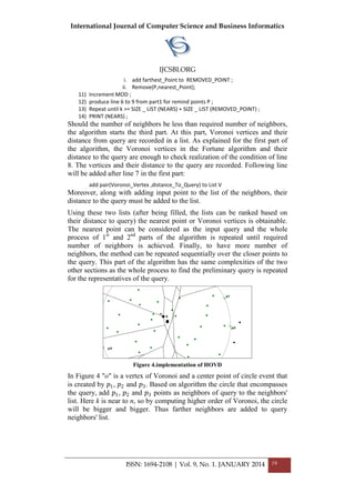
4.1 HOV-kNN algorithm
After describing our algorithm in the previous paragraph briefly, we will
elaborate it formally in this section. When the first order Voronoi diagram is
constructed, some of the query neighbors can be obtained in complexity of
the Fortune algorithm (i.e.𝑂(𝑛𝑙𝑜𝑔𝑛)). This fact forms the first step of our
algorithm. When the discovered circle event in HandleCircleEvent of the
Fortune algorithm is real (initialized by the variable “check” in line 6 of the
algorithm, and by default function HandleCircleEvent returns “true” when
circle even is real) the query distance is measured from center of the circle.
Moreover, when the condition in line 7.i of the algorithm is true, the three
points that constitute the circle are added to NEARS list if not been added](https://image.slidesharecdn.com/vol9no1-january2014-171208072155/85/Vol-9-No-1-January-2014-20-320.jpg)
![International Journal of Computer Science and Business Informatics
IJCSBI.ORG
ISSN: 1694-2108 | Vol. 9, No. 1. JANUARY 2014 18
before (function PUSH-TAG (p) shows whether it is added to NEAR list or
not).
1) Input : q , a query
2) Output: list NEARS, k nearest neighbors.
3) Procedure :
4) Initialization :
5) NEARS ={}, K nearest neighbors
, Check = false, MOD = 0, V = {} (hold Voronoipoints( ;
6) Check = HandleCircleEvent()
7) If check= true, then -- detect a true circle event.
i) If distance(q , o) < r Then
(1) If PUSH-TAG(p1) = false , Then
(a) add p1 to NEARS
(2) If PUSH-TAG (p2) = false , Then
(a) add p2 to NEARS
ii) If PUSH-TAG(p3) = false, Then
(a) add p3 to NEARS
Real circle events are discovered up to this point and the points that
constitute the events are added to neighbor list of the query. As pointed out
earlier, the preferred result is obtained, if “k” inputs are equal or lesser than
number of the obtained neighbors a𝑂(𝑛𝑙𝑜𝑔𝑛)complexity.
8) if SIZE (NEARS) >= k , then
a. sort (NERAS ) - - sort NEARS by distance
b. for i = 1 to k
i. print (NEARS);
9) else if SIZE (NEARS) = k
ii. print(NEARS);
The algorithm enters the second step if the conditions of line 8 and 9 in the
first part are not met. The second part compute vertices of Voronoi
sequentially, so that the obtained vertices are HOV vertex. Under sequential
method for developing HOV [12], the vertices of the HOV are obtained by
omitting the closer neighbors. Here, however, to find more neighbors
through sequential method, loop one of the closest neighbor and loop one of
the farthest neighbor are deleted alternatively from the set of the point. This
leads to new circles that encompass the query. Afterward, the same
calculations described in section one are carried out for the remaining points
(the removed neighbors are recorded a list named REMOVED_POINTS).
The calculations are carried out until the loop condition in line 5 is met.
10) Else if (SIZE(NEARS) < k )
c. if mod MOD 2 = 0 , then
i. add nearest_Point to REMOVED_POINT ;
ii. Remove(P,nearest_Point);
d. if mod MOD 2 = 1 , then](https://image.slidesharecdn.com/vol9no1-january2014-171208072155/85/Vol-9-No-1-January-2014-21-320.jpg)
![International Journal of Computer Science and Business Informatics
IJCSBI.ORG
ISSN: 1694-2108 | Vol. 9, No. 1. JANUARY 2014 20
4.2 The complexity of HOV-kNN
As mentioned before, HOV-kNN algorithm has a time complexity lesser
than the time complexity of D.T. Lee’s algorithm. To show this fact,
consider the presented algorithm in the previous section. Line 13 explains
that the main body of algorithm must be repeated k times in which "k" are
the number of neighbors that should be found. In each repetition one of the
query’s neighbors are detected by algorithm and subsequently eliminated
from dataset. The principle part of our algorithm that is the most time
consuming part too is between lines 6 and 9. This line recalls modified
Fortune algorithm which has a time complexity𝑂(𝑛𝑙𝑜𝑔𝑛). Therefore the
overall complexity of our algorithm will be:
𝑂 𝑛𝑙𝑜𝑔𝑛
𝑘
𝑖=1
= 𝑂 𝑛𝑙𝑜𝑔𝑛 1
𝑘
𝑖=0
= 𝑘𝑂 𝑛𝑙𝑜𝑔𝑛 = 𝑂 𝑘𝑛𝑙𝑜𝑔𝑛 (2)
In comparison to the algorithm introduced in [12] (which has a time
complexity𝑂(𝑘2
𝑛𝑙𝑜𝑔𝑛)) our algorithm is faster k times. The main reason of
this difference is that Lee’s algorithm completely computes the HOVD,
while ours exploits a fraction of HOVD construction process. In term of
space complexity, the space complexity of our algorithm is the same as the
space complexity of Fortune algorithm: 𝑂(𝑛).
5. IMPLEMENTATION AND EVALUATION
This section introduces the results of the HOV-kNN algorithm and
compares the results with other algorithms. We use Voronoi diagram which
is used to find k nearest neighbor points that is less complicated. The
proposed algorithm was implemented using C++. For maintaining data
points vector data structure, which is one of the C++ standard libraries, was
used. The input data points used in the program test were adopted randomly.
To reach preferred data distribution, not too close/far points, they were
generated under specific conditions. For instance, for 100 input points, the
point generation range is 0-100 and for 500 input points the range is 0-500.
To ensure accuracy and validity of the output, a simple kNN algorithm was
implemented and the outputs of the two algorithms were compared (equal
input, equal query). Outputs evaluation was also carried out sequentially and
the outputs were stored in two separate files. Afterward, to compare
similarity rate, the two files were used as input to another program.
The evaluation was also conducted in two steps. First the parameter “k” was
taken as a constant and the evaluation was performed using different points
of data as input. As pictured in Figure 5, accuracy of the algorithm is more
than 90%. In this diagram, the number of inputs in dataset varies between 10
and 100000. At the second step, the evaluation was conducted with different
values of k, while the number of input data was stationary. Accuracy of the
algorithm was obtained 74% while “k” was between 10 and 500 (Figure 6).](https://image.slidesharecdn.com/vol9no1-january2014-171208072155/85/Vol-9-No-1-January-2014-23-320.jpg)

![International Journal of Computer Science and Business Informatics
IJCSBI.ORG
ISSN: 1694-2108 | Vol. 9, No. 1. JANUARY 2014 22
REFERENCES
[1] Lifshits, Y.Nearest neighbor search: algorithmic perspective, SIGSPATIAL Special.
Vol. 2, No 2, 2010, 12-15.
[2] Shakhnarovich, G., Darrell, T., and Indyk, P.Nearest Neighbor Methods in Learning
and Vision: Theory and Practice, The MIT Press, United States, 2005.
[3] Andoni, A.Nearest Neighbor Search - the Old, the New, and the Impossible, Doctor of
Philosophy, Electrical Engineering and Computer Science, Massachusetts Institute of
Technology,2009.
[4] Bhatia, N., and Ashev, V. Survey of Nearest Neighbor Techniques, International
Journal of Computer Science and Information Security, Vol. 8, No 2, 2010, 1- 4.
[5] Dhanabal, S., and Chandramathi, S. A Review of various k-Nearest Neighbor Query
Processing Techniques, Computer Applications, Vol. 31, No 7, 2011, 14-22.
[6] Hajebi, K., Abbasi-Yadkori, Y., Shahbazi, H., and Zhang, H.Fast approximate nearest-
neighbor search with k-nearest neighbor graph, In Proceedings of 22 international joint
conference on Artificial Intelligence, Vol. 2 (IJCAI'11), Toby Walsh (Ed.), 2011, 1312-
1317.
[7] Fukunaga, K. Narendra, P. M. A Branch and Bound Algorithm for Computing k-
Nearest Neighbors, IEEE Transactions on Computer,Vol. 24, No 7, 1975, 750-753.
[8] Song, Z., Roussopoulos, N. K-Nearest Neighbor Search for Moving Query Point, In
Proceedings of the 7th International Symposium on Advances in Spatial and Temporal
Databases (Redondo Beach, California, USA), Springer-Verlag, 2001, 79-96.
[9] Güting, R., Behr, T., and Xu, J. Efficient k-Nearest Neighbor Search on moving object
trajectories, The VLDB Journal 19, 5, 2010, 687-714.
[10]Frentzos, E., Gratsias, K., Pelekis, N., and Theodoridis, Y.Algorithms for Nearest
Neighbor Search on Moving Object Trajectories, Geoinformatica 11, 2, 2007,159-193.
[11]Berg, M. , Cheong, O. , Kreveld, M., and Overmars, M.Computational Geometry:
Algorithms and Applications, Third Edition, Springer-Verlag, 2008.
[12]Lee, D. T. On k-Nearest Neighbor Voronoi Diagrams in the Plane, Computers, IEEE
Transactions on Volume:C-31, Issue:6, 1982, 478–487.
[13]Fortune, S. A sweep line algorithm for Voronoi diagrams, Proceedings of the second
annual symposium on Computational geometry, Yorktown Heights, New York, United
States, 1986, 313–322.
[14]Meyerhenke, H. Constructing Higher-Order Voronoi Diagrams in Parallel,
Proceedings of the 21st European Workshop on Computational Geometry, Eindhoven,
The Netherlands, 2005, 123-126.
[15]Gao, Y., Zheng, B., Chen, G., and Li, Q. Algorithms for constrained k-nearest neighbor
queries over moving object trajectories, Geoinformatica 14, 2 (April 2010 ), 241-276.
This paper may be cited as:
Abbasifard, M. R., Naderi, H. and Mirjalili, M., 2014. HOV-kNN: A New
Algorithm to Nearest Neighbor Search in Dynamic Space. International
Journal of Computer Science and Business Informatics, Vol. 9, No. 1, pp.
12-22.](https://image.slidesharecdn.com/vol9no1-january2014-171208072155/85/Vol-9-No-1-January-2014-25-320.jpg)
![International Journal of Computer Science and Business Informatics
IJCSBI.ORG
ISSN: 1694-2108 | Vol. 9, No. 1. JANUARY 2014 24
2. RELATED WORKS
Malware is a malicious piece of software which is designed to damage the
computer system & interrupt its typical working. Fundamentally, malware is
a short form of Malicious Software. Mobile malware is a malicious software
aiming mobile phones instead of traditional computer system. With the
evolution of mobile phones, mobile malware started its evolution too [1-4].
When propagation medium is taken into account, mobile viruses are of three
types: Bluetooth-based virus, SMS-based virus, and FM RDS based virus
[5-9]. A BT-based virus propagates through Bluetooth & Wi-Fi which has
regional impact [5], [7], and [8]. On the contrary, SMS-based virus follows
long-range spreading pattern & can be propagated through SMS & MMS
[5], [6], [8]. FM RDS based virus uses RDS channel of mobile radio
transmitter for virus propagation [9]. Our work addresses the effect of
operational behavior of user & mobility of a device in virus propagation.
There are several methods of malware detection viz. static method, dynamic
method, cloud-based detection method, battery life monitoring method,
application permission analysis, enforcing hardware sandbox etc. [10-18]. In
addition to work given in [10-18], our work addresses pros and cons of each
malware detection method. Along with the study of virus propagation &
detection mechanisms, methods of restraining virus propagation are also
vital. A number of proactive & reactive malware control strategies are given
in [5], [10].
3. EVOLUTION OF MOBILE MALWARE
Although, first mobile malware, ‘Liberty Crack’, was developed in year
2000, mobile malware evolved rapidly during years 2004 to 2006 [1].
Enormous varieties of malicious programs targeting mobile devices were
evolved during this time period & are evolving till date. These programs
were alike the malware that targeted traditional computer system: viruses,
worms, and Trojans, the latter including spyware, backdoors, and adware.
At the end of 2012, there were 46,445 modifications in mobile malware.
However, by the end of June 2013, Kaspersky Lab had added an aggregate
total of 100,386 mobile malware modifications to its system [2]. The total
mobile malware samples at the end of December 2013 were 148,778 [4].
Moreover, Kaspersky labs [4] have collected 8,260,509 unique malware
installation packs. This shows that there is a dramatic increase in mobile
malware. Arrival of ‘Cabir’, the second most mobile malware (worm)
developed in 2004 for Symbian OS, dyed-in-the-wool the basic rule of
computer virus evolution. Three conditions are needed to be fulfilled for
malicious programs to target any particular operating system or platform:](https://image.slidesharecdn.com/vol9no1-january2014-171208072155/85/Vol-9-No-1-January-2014-27-320.jpg)
![International Journal of Computer Science and Business Informatics
IJCSBI.ORG
ISSN: 1694-2108 | Vol. 9, No. 1. JANUARY 2014 25
The platform must be popular: During evolution of ‘Cabir’, Symbian
was the most popular platform for smart phones. However,
nowadays it is Android, that is most targeted by attackers. These
days’ malware authors continue to ponder on the Android platform
as it holds 93.94% of the total market share in mobile phones and
tablet devices.
There must be a well-documented development tools for the
application: Nowadays every mobile operating system developers
provides a software development kit & precise documentation which
helps in easy application development.
The presence of vulnerabilities or coding errors: During the
evolution of ‘Cabir’, Symbian had number of loopholes which was
the reason for malware intrusion. In this day and age, same thing is
applicable for Android [3].
Share of operating system plays a crucial role in mobile malware
development. Higher the market share of operating system, higher is the
possibility of malware infection. The pie chart below illustrates the
operating system (platform) wise mobile malware distribution [4]:
Figure 1. OS wise malware distribution](https://image.slidesharecdn.com/vol9no1-january2014-171208072155/85/Vol-9-No-1-January-2014-28-320.jpg)
![International Journal of Computer Science and Business Informatics
IJCSBI.ORG
ISSN: 1694-2108 | Vol. 9, No. 1. JANUARY 2014 26
4. MOBILE MALWARE PROPAGATION
There are 3 communication channels through which malware can propagate.
They are: SMS / MMS, Bluetooth / Wi-Fi, and FM Radio broadcasts.
4.1 SMS / MMS
Viruses that use SMS as a communication media can send copies of
themselves to all phones that are recorded in victim’s address book. Virus
can be spread by means of forwarding photos, videos, and short text
messages, etc. For propagation, a long-range spreading pattern is followed
which is analogous to the spreading of computer viruses like worm
propagation in e-mail networks [6]. For accurate study of SMS-based virus
propagation, one needs to consider certain operational patterns, such as
whether or not users open a virus attachment. Hence, the operational
behavior of users plays a vital role in SMS-based virus propagation [8].
4.1.1 Process of malware propagation
If a phone is infected with SMS-based virus, the virus regularly sends its
copies to other phones whose contact number is found in the contact list of
the infected phone. After receiving such distrustful message from others,
user may open or delete it as per his alertness. If user opens the message, he
is infected. But, if a phone is immunized with antivirus, a newly arrived
virus won’t be propagated even if user opens an infected message.
Therefore, the security awareness of mobile users plays a key role in SMS-
based virus propagation.
Same process is applicable for MMS-based virus propagation whereas
MMS carries sophisticated payload than that of SMS. It can carry videos,
audios in addition to the simple text & picture payload of SMS.
4.2 Bluetooth/ Wi-Fi
Viruses that use Bluetooth as a communication channel are local-contact
driven viruses since they infect other phones within its short radio range.
BT-based virus infects individuals that are homogeneous to sender, and each
of them has an equal probability of contact with others [7]. Mobility
characteristics of user such as whether or not a user moves at a given hour,
probability to return to visited places at the next time, traveling distances of
a user at the next time etc. are need to be considered [8].
4.2.1 Process of malware propagation
Unlike SMS-based viruses, if a phone is infected by a BT-based virus, it
spontaneously & atomically searches another phone through available
Bluetooth services. Within a range of sender mobile device, a BT-based
virus is replicated. For that reason, users’ mobility patterns and contact](https://image.slidesharecdn.com/vol9no1-january2014-171208072155/85/Vol-9-No-1-January-2014-29-320.jpg)
![International Journal of Computer Science and Business Informatics
IJCSBI.ORG
ISSN: 1694-2108 | Vol. 9, No. 1. JANUARY 2014 27
frequency among mobile phones play crucial roles in BT-based virus
propagation.
Same process is followed for Wi-Fi where Wi-Fi is able to carry high
payload in large range than that of BT.
4.3 FM-RDS
Several existing electronic devices do not support data connectivity facility
but include an FM radio receiver. Such devices are low-end mobile phones,
media players, vehicular audio systems etc. FM provides FM radio data
system (RDS), a low-rate digital broadcast channel. It is proposed for
delivering simple information about the station and current program, but it
can also be used with other broad range of new applications and to enhance
existing ones as well [9].
4.3.1 Process of malware propagation
The attacker can attack in two different ways. The first way is to create a
seemingly benign app and upload it to popular app stores. Once the user
downloads & installs the app, it will contact update server & update its
functionality. This newly added malicious functionality decodes and
assembles the payload. At the end, the assembled payload is executed by the
Trojan app to uplift privileges of attacked device & use it for malicious
purpose. Another way is, the attacker obtains a privilege escalation exploit
for the desired target. As RDS protocol has a limited bandwidth, we need to
packetize the exploit. Packetization is basically to break up a multi-kilobyte
binary payload into several smaller Base64 encoded packets. Sequence
numbers are attached for proper reception of data at receiver side. The
received exploit is executed. In this way the device is infected with malware
[9].
5. MOBILE MALWARE DETECTION TECHNIQUE
Once the malware is propagated, malware detection is needed to be carried
out. In this section, various mobile malware detection techniques are
explained.
5.1 Static Analysis Technique
As the name indicates, static analysis is to evaluate the application without
execution [10-11]. It is an economical as well as fast approach to detect any
malevolent characteristics in an application without executing it. Static
analysis can be used to cover static pre-checks that are performed before the
application gets an entry to online application markets. Such application
markets are available for most major smartphone platforms e.g. ‘Play store’
for Android, ‘Store’ for windows operating system. . These extended pre-](https://image.slidesharecdn.com/vol9no1-january2014-171208072155/85/Vol-9-No-1-January-2014-30-320.jpg)
![International Journal of Computer Science and Business Informatics
IJCSBI.ORG
ISSN: 1694-2108 | Vol. 9, No. 1. JANUARY 2014 28
checks enhance the malware detection probabilities and therefore further
spreading of malware in the online application stores can be banned. In
static analysis, the application is investigated for apparent security threats
like memory corruption flaws, bad code segment etc. [10], [12].
5.1.1 Process of malware detection
If the source code of application is available, static analysis tools can be
directly used for further examination of code.
But if the source code of the application is not available then executable app
is converted back to its source code. This process is known as
disassembling. Once the application is disassembled, feature extraction is
done. Feature extraction is nothing but observing certain parameters viz.
system calls, data flow, control flow etc. Depending on the observations,
anomaly is detected. In this way, application is categorized as either benign
or malicious.
Pros: Economical and fast approach of malware detection.
Cons: Source codes of applications are not readily available. And
disassembling might not give exact source codes.
Figure 2. Static Analysis Technique
5.1.2 Example
Figure 2 shows the malware detection technique proposed by Enck et al.
[12] for Android. Application’s installation image (.apk) is used as an input
to system. Ded, a Dalvik decompiler, is used to dissemble the code. It](https://image.slidesharecdn.com/vol9no1-january2014-171208072155/85/Vol-9-No-1-January-2014-31-320.jpg)
![International Journal of Computer Science and Business Informatics
IJCSBI.ORG
ISSN: 1694-2108 | Vol. 9, No. 1. JANUARY 2014 29
generates Java source code from .apk image. Feature extraction is done by
using Fortify SCA. It is a static code analysis suite that provides four types
of analysis; control flow analysis, data flow analysis, structural analysis, and
semantic analysis. It is used to evaluate the recovered source code &
categorize the application as either benign or malicious.
5.2 Dynamic Analysis Technique
Dynamic analysis comprises of analyzing the actions performed by an
application while it is being executed. In dynamic analysis, the mobile
application is executed in an isolated environment such as virtual machine
or emulator, and the dynamic behavior of the application is monitored [10],
[11], [13]. There are various methodologies to perform dynamic analysis
viz. function call monitoring, function parameter analysis, Information flow
tracking, instruction trace etc. [13].
5.2.1 Process of malware detection
Dynamic analysis process is quite diverse than the static analysis. In this,
the application is installed in the standard Emulator. After installation is
done, the app is executed for a specific time and penetrated with random
user inputs. Using various methodologies mentioned in [13], the application
is examined. On the runtime behavior, the application is either classified as
benign or malicious.
Pros: Comprehensive approach of malware detection. Most of the malwares
is got detected in this technique.
Cons: Comparatively complex and requires more resources.
Figure 3. Dynamic Analysis Technique](https://image.slidesharecdn.com/vol9no1-january2014-171208072155/85/Vol-9-No-1-January-2014-32-320.jpg)
![International Journal of Computer Science and Business Informatics
IJCSBI.ORG
ISSN: 1694-2108 | Vol. 9, No. 1. JANUARY 2014 30
5.2.2 Example
Figure 3 shows Android Application Sandbox (AASandbox) [14], the
dynamic malware detection technique proposed by Blasing et al. for
Android. It is a two-step analysis process comprising of both static &
dynamic analysis. The AASandbox first implements a static pre-check,
followed by a comprehensive dynamic analysis. In static analysis, the
application image binary is disassembled. Now the disassembled code is
used for feature extraction & to search for any distrustful patterns. After
static analysis, dynamic analysis is performed. In dynamic analysis, the
binary is installed and executed in an AASandbox. ‘Android Monkey’ is
used to generate runtime inputs. System calls are logged & log files are
generated. This generated log file will be then summarized and condensed to
a mathematical vector for better analysis. In this way, application is
classified as either benign or malicious.
5.3 Cloud-based Analysis Technique
Mobile devices possess limited battery and computation. With such
constrained resource availability, it is quite problematic to deploy a full-
fledged security mechanism in a smartphone. As data volume increases, it is
efficient to move security mechanisms to some external server rather than
increasing the working load of mobile device [10], [15].
5.3.1 Process of malware detection
In the cloud-based method of malware detection, all security computations
are moved to the cloud that hosts several replicas of the mobile phones
running on emulators & result is sent back to mobile device. This increases
the performance of mobile devices.
Pros: Cloud holds ample resources of each type that helps in more
comprehensive detection of malware.
Cons: Extra charges to maintain cloud and forward data to cloud server.
5.3.2 Example
Figure 4 shows Paranoid Android (PA), proposed by Portokalidis et al. [15].
Here, security analysis and computations are moved to a cloud (remote
server). It consists of 2 different modules, a tracer & replayer. A tracer is
located in each smart phone. It records all necessary information that is
required to reiterate the execution of the mobile application on remote
server. The information recorded by tracer is first filtered & encoded. Then
it is stored properly and synchronized data is sent to replayer over an
encrypted channel. Replayer is located in the cloud. It holds the replica of
mobile phone running on emulator & records the information communicated
by tracer. The replayer replays the same execution on the emulator, in the](https://image.slidesharecdn.com/vol9no1-january2014-171208072155/85/Vol-9-No-1-January-2014-33-320.jpg)
![International Journal of Computer Science and Business Informatics
IJCSBI.ORG
ISSN: 1694-2108 | Vol. 9, No. 1. JANUARY 2014 31
cloud. Cloud, the remote server, owns abundant resources to perform
multifarious analysis on the data collected from tracer. During the replay,
numerous security analyses such as dynamic malware analysis, memory
scanners, system call tracing, call graph analysis[15] etc. are performed
rather there is no limit on the number of attack detection techniques that we
can be applied in parallel.
Figure 4. Cloud-based Detection Technique
5.4 Monitoring Battery Consumption
Monitoring battery life is a completely different approach of malware
detection compared to other ones. Usually smartphones possess limited
battery capacity and need to be used judiciously. The usual user behavior,
existing battery state, signal strength and network traffic details of a mobile
is recorded over time and this data can be effectively used to detect hidden
malicious activities. By observing current energy consumption such
malicious applications can indeed be detected as they are expected to take in
more power than normal regular usage. Though, battery power consumption
is one of the major limitations of mobile phones that limit the complexity of
anti-malware solutions. A quite remarkable work is done in this field. The
introductory exploration in this domain is done by Jacoby and Davis [16].
5.4.1 Process of malware detection
After malware infection, that greedy malware keeps on repeating itself. If
the mean of propagation is Bluetooth then the device continuously scans for](https://image.slidesharecdn.com/vol9no1-january2014-171208072155/85/Vol-9-No-1-January-2014-34-320.jpg)
![International Journal of Computer Science and Business Informatics
IJCSBI.ORG
ISSN: 1694-2108 | Vol. 9, No. 1. JANUARY 2014 32
adjacent Bluetooth-enabled devices which in turn consume a remarkable
amount of power. This time-domain data of power consumption collected
over a period of time is transformed into frequency-domain data &
represented as dominant frequencies. The malwares are identified from
these certain dominant frequencies.
Pros: Economical and novel approach of malware detection.
Cons: Because of multi-functionality of smart phones, power consumption
model of smart phone could not be accurately defined.
5.4.2 Example
Recent work by Liu et al. [17] proposed another detection technique by
comparing the compressed sequences of the power consumption value in
each time interval. They defined a user-centric power model that relies on
user actions. User actions such as duration & frequency of calls, number of
SMS, network usage are taken into account. Their work uses machine
learning techniques to generate rules for malware detection.
5.5 Application Permission Analysis
With the advancements in mobile phone technology, users have started
downloading third party application. These applications are available in
third party application stores. While developing any application, application
developers need to take required permissions from device in order to make
the application work on that device. Permissions hold a crucial role in
mobile application development as they convey the intents and back-end
activities of the application to the user. Permissions should be precisely
defined & displayed to the user before the application is installed. Though,
some application developers hide certain permissions from user & make the
application vulnerable & malicious application.
5.5.1 Process of malware detection
Security configuration of an application is extracted. Permissions taken by
an application are analyzed. If application has taken any unwanted
applications then it is categorized as malicious.
Pros: Fewer resources are required compared to other techniques.
Cons: Analyzing only the permissions request is not adequate for mobile
malware detection; it needs to be done in parallel with static and/or dynamic
analysis.
5.5.2 Example
Kirin, proposed by Enck et al. (2009) [18] is an application certification
system for Android. During installation, Kirin crisscrosses the application
permissions. It extracts the security configurations of the application](https://image.slidesharecdn.com/vol9no1-january2014-171208072155/85/Vol-9-No-1-January-2014-35-320.jpg)
![International Journal of Computer Science and Business Informatics
IJCSBI.ORG
ISSN: 1694-2108 | Vol. 9, No. 1. JANUARY 2014 33
&checks it against the templates i.e. security policy rules already defined by
Kirin. If any application becomes unsuccessful to clear all the security
policy rules, Kirin either deletes the application or alerts the user for
assistance [18].
6. MOBILE MALWARE CONTROL STRATEGIES
Basically, there are two types of malware control strategies, viz. proactive &
reactive control. In proactive malware control strategy, malware is mitigated
before its propagation. Proper set of preventive measures is used for this
purpose. While, in reactive malware control strategy, malware is first
propagated and then a reaction is taken upon malware contamination.
6.1 Proactive Malware Control Strategy
Here are some of the proactive malware control techniques given in [10];
however, users’ own security awareness plays a crucial role.
Install a decent mobile security application i.e. antivirus.
Always download apps from trusted official application markets.
Before downloading any app, do read the reviews and ratings of the
app. During installation, always remember to read the permissions
requested by the app and if it appears doubtful don’t install it.
Always keep installed apps up-to-date.
Turn-off Wi-Fi, Bluetooth, and other short range wireless
communication media when not to be used. Stay more conscious
when connecting to insecure public Wi-Fi networks & accepting
Bluetooth data from unknown sender.
When confidential data is to be stored in the mobile phone, encrypt it
before storing and set a password for access. Do regular back-ups.
Assure that the sensitive information is not cached locally in the
mobile phone.
Always keep an eye on the battery life, SMS and call charges, if
found any few and far between behaviors, better go for an in-depth
check on the recently installed applications.
During internet access, don’t click on links that seem suspicious or
not trustworthy.
Finally, in case of mobile phone theft, delete all contacts,
applications, and confidential data remotely.
6.2Reactive Malware Control Strategy
When the malware is detected then the control strategy is implemented, is
the working principle of reactive malware control strategy. Antivirus
solution comes under proactive malware control, however when a new](https://image.slidesharecdn.com/vol9no1-january2014-171208072155/85/Vol-9-No-1-January-2014-36-320.jpg)
![International Journal of Computer Science and Business Informatics
IJCSBI.ORG
ISSN: 1694-2108 | Vol. 9, No. 1. JANUARY 2014 34
malware is found, antivirus updates for that malware are implemented and
forwarded to mobile phones, is a part of reactive malware control. This is
known as adaptive patch dissemination.
Adaptive Patch Dissemination
A pre-immunization like antivirus is used to protect networks before virus
propagation. However, in reality, we first detect certain viruses and then
update antivirus, known as patches. These patches are forwarded into
networks only after these viruses have already propagated. Network
bandwidth limits the speed with which the security notifications or patches
can be sent to all users simultaneously. Therefore, a new strategy namely
adaptive dissemination strategy is developed. It is based on the Autonomy
Oriented Computing (AOC) methodology which helps to send security
notifications or patches to most of phones with a relatively lower
communication cost. The AOC is used to search a set of the highly
connected phones with large communication abilities in a mobile network
[5].
7. CONCLUSION
Rapid growth in smart phone development resulted in evolution of mobile
malware. Operating system shares’ plays crucial role in malware evolution.
SMS/MMS is the fastest way of mobile malware propagation as it has no
geographical boundary like BT/Wi-Fi. FM-RDS is still evolving. Among all
malware detection techniques, static malware detection is performed first
during pre-checks. Later dynamic analysis is performed and can be
combined with application permission analysis. Cloud-based analysis is
more comprehensive approach as it uses external resources to perform
malware detection and can perform more than one type of analysis
simultaneously. Proactive control strategy is used to control malware before
its propagation while reactive control strategy is used after malware is
propagated.
REFERENCES
[1] La Polla, M., Martinelli, F., & Sgandurra, D. (2012). A survey on security for mobile
devices. IEEE Communications Surveys & Tutorials, 15(1), 446 – 471.
[2] Kaspersky Lab IT Threat Evolution: Q2 2013. (2013). Retrieved from
http://www.kaspersky.co.in/about/news/virus/2013/kaspersky_lab_it_threat_evolution_q2_
2013.
[3] Kaspersky Security Bulletin 2013: Overall statistics for 2013. (2013 December).
Retrieved from
http://www.securelist.com/en/analysis/204792318/Kaspersky_Security_Bulletin_2013_Ove
rall_statistics_for_2013.](https://image.slidesharecdn.com/vol9no1-january2014-171208072155/85/Vol-9-No-1-January-2014-37-320.jpg)
![International Journal of Computer Science and Business Informatics
IJCSBI.ORG
ISSN: 1694-2108 | Vol. 9, No. 1. JANUARY 2014 35
[4] Maslennikov, D. Mobile Malware Evolution: Part 6. (2013 February). Retrieved from
http://www.securelist.com/en/analysis/ 204792283/Mobile_Malware_Evolution_Part_6.
[5] Gao, C., and Liu, J. (2013). Modeling and restraining mobile virus propagation. IEEE
transactions on mobile computing, 12(3), 529-541.
[6] Gao, C. and Liu, J. (2011). Network immunization and virus propagation in Email
networks: Experimental evaluation and analysis. Knowledge and information systems,
27(2), 253-279.
[7] Yan, G., and Eidenbenz, S. (2009, March). Modeling propagation dynamics of
Bluetooth worms (extended version). IEEE transactions on Mobile Computing, 8(3), 353-
368.
[8] Gonzalez, M., Hidalgo, C., and Barabasi, A. (2008). Understanding individual human
mobility patterns. Nature, 453(7196), 779-782.
[9] Fernandes, E., Crispo, B., Conti, M. (2013, June). FM 99.9, Radio virus: Exploiting
FM radio broadcasts for malware deployment. Transactions on information forensics and
security, 8(6), 1027-1037.
[10] Chandramohan, M., and Tan, H. (2012). Detection of mobile malware in the wild.
IEEE computer society, 45(9), 65-71.
[11] Yan, Q., Li, Y., Li, T., and Deng, R. (2009). Insights into malware detection and
prevention on mobile phones. Springer-Verlag Berlin Heidelberg, SecTech 2009, 242–249.
[12] Enck, W., Octeau, D., Mcdaniel, P., and Chaudhuri, S. (2011 August). A study of
android application security. The 20th Usenix security symposium.
[13] Egele, M., Scholte, T., Kirda, E., Kruegel, C. (2012 February). A survey on automated
dynamic malware-analysis techniques and tools. ACM-TRANSACTION, 4402(06), 6-48.
[14] Blasing, T., Batyuk, L., Schmidt, A., Camtepe, S., and Albayrak, S. (2010). An
android application sandbox system for suspicious software detection. 5th International
Conference on Malicious and Unwanted Software.
[15] Portokalidis, G., Homburg, P., Anagnostakis, K., Bos, H. (2010 December). Paranoid
android: Versatile protection for smartphones. ACSAC'10.
[16] Jacoby, G. (2004). Battery-based intrusion detection. The Global Telecommunications
Conference.
[17] Liu, L., Yan, G., Zhang, X., and Chen, S. (2009). Virusmeter: Preventing your
cellphone from spies. RAID, 5758, 244-264.
[18] Enck, W., Ongtang, M., and Mcdaniel, P. (2009 November). On lightweight mobile
phone application certification. 16th ACM Conference on Computer and Communications
Security.
This paper may be cited as:
Mohite, S. and Sonar, R. S., 2014. A Survey on Mobile Malware: A War
without End. International Journal of Computer Science and Business
Informatics, Vol. 9, No. 1, pp. 23-35.](https://image.slidesharecdn.com/vol9no1-january2014-171208072155/85/Vol-9-No-1-January-2014-38-320.jpg)
![International Journal of Computer Science and Business Informatics
IJCSBI.ORG
ISSN: 1694-2108 | Vol. 9, No. 1. JANUARY 2014 37
Modeling Language (UML) is now widely accepted as the standard
modeling language for software construction and is gaining wide
acceptance. The class diagram in its core view provides the backbone for
any modeling effort and has well formed semantics.
2. BACKGROUND STUDY
Alexander Egyed [4, 5] presents an automated approach for detecting and
tracking inconsistencies in real time and to automatically identify changes in
various models that affect the consistency rules. The approach observes the
behavior of consistency rules to understand how they affect the model.
Techniques for efficiently detecting inconsistencies in UML Models
identifying the changes required to fix problems are analyzed. The work
describes a technique for automatically generating a set of concrete changes
for fixing inconsistencies and providing information about the impact of
each change on all consistency rules. The approach is integrated with the
design tool IBM Rational Rose TM. Muhammad Usman [9] presents a
survey of UML consistency checking techniques by analyzing various
parameters and constructs an analysis table. The analysis table helps
evaluate existing consistency checking techniques and concludes that most
of the approaches validate intra and inter level consistencies between UML
models by using monitoring strategy. UML class, sequence, and state chart
diagrams are used in most of the existing consistency checking techniques.
Alexander Egyed demonstrates [3] that a tool can assist the designer in
discovering unintentional side effects, locating choices for fixing
inconsistencies, and then in changing the design model.
The paper examines the impact of changes on UML design models [10] and
explores the methodology to discover the negative side effects of design
changes, and to predict the positive and negative impact of these choices.
Alexander Egyed [1, 2] presents an approach for quickly, correctly, and
automatically deciding the consistency rules required to evaluate when a
model changes. The approach does not require consistency rules with
special annotations. Instead, it treats consistency rules as black-box entities
and observes their behavior during their evaluation to identify the different
types of model elements they access.
Christian Nentwich [6, 7] presents a repair framework for inconsistent
distributed documents for generating interactive repairs from full first order
logic formulae that constrain the documents. A full implementation of the
components as well as their application to the UML and related
heterogeneous documents such as EJB deployment descriptors are
presented. This approach can be used as an infrastructure for building high
domain specific frameworks. Researchers have focused to remove](https://image.slidesharecdn.com/vol9no1-january2014-171208072155/85/Vol-9-No-1-January-2014-40-320.jpg)
![International Journal of Computer Science and Business Informatics
IJCSBI.ORG
ISSN: 1694-2108 | Vol. 9, No. 1. JANUARY 2014 38
inconsistencies in few UML Models. The work proposed in [11] attempts to
address and detect inconsistencies in UML Models like Class diagram, Use
case diagram, Sequence diagram and so on. A survey exploring the impact
of model driven software development is given in [12]. Change in impact
analysis, consistency management and uncertainty management,
inconsistency detection and resolution rules are dealt in the work.
3. FRAME WORK OF THE PROPOSED WORK
Figure 1. Framework of the proposed work
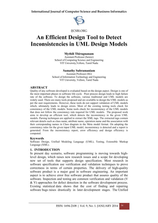
4. DETAILED DESCRIPTION OF THE PROPOSED WORK
The framework of the proposed work is given in Figure 1.
4.1. Converting UML model into XML file
An UML design diagram does not support to directly detect the
inconsistency which is practically impossible. UML model is converted into
XML file for detecting the inconsistency in the model. UML models such as
use case diagram, class diagram and sequence diagram can be taken as input
for this tool. The final output of this module is XML file which is used
further to detect the inconsistency. The snapshot of getting input file is
shown in Figure 2.
Extract the XML tags
Apply parsing
Technique
Applying consistency
rules
Detect Inconsistency in the
given input
Generate the
Inconsistency report
Select UML model Convert UML model into
XML file](https://image.slidesharecdn.com/vol9no1-january2014-171208072155/85/Vol-9-No-1-January-2014-41-320.jpg)
![International Journal of Computer Science and Business Informatics
IJCSBI.ORG
ISSN: 1694-2108 | Vol. 9, No. 1. JANUARY 2014 39
Procedure used:
Convert the chosen input design into a XML file
Select Input File Export as XML file VP-UML project
Select the diagram that needs to be exported
Select the location for exported file to be stored
The input file is read from the user to carry out further process (Figure 2).
Here, Use Case Diagram is read as input file. The input diagram is stored
as XML file and passed as the input to the next process that extracts the
XML tags.
4.2. Extracting the XML tags and applying the parsing technique
From the XML file, the XML tags are extracted. The parsing technique is
applied on the XML tags to identify the related information of the given
model which is in Meta model format [3]. For example, in class diagram,
the class name, its attributes and methods are identified. All the related
information of the given input model is extracted.
Procedure used:
Open the XML file
Copy the file as text file
Split the tag into tokens Extract the relevant information about
the diagram
Save the extracted result in a file.
Figure 3 & 4 describes the above mentioned procedure. The XML file is
considered as the input for this step. This method adopts the tokenizer
concept to split the tags and store.
4.3. Detecting the design inconsistency:
The consistency rules [8, 10] are applied on the related information of the
given input design diagram to detect the inconsistency. The related
information which does not satisfy the rule has design inconsistency for the
given input model. All possible inconsistency is detected as described
below. Figure 5 shows the inconsistencies in given use case diagram.
4.3.1. Consistency rule for the Class Diagram:
Visibility of a member should be given.
Visibility of all attributes should be private.
Visibility of all methods should be public.
Associations should have cardinality relationship.
When one class depends on another class, there should be class
interfaces notation.](https://image.slidesharecdn.com/vol9no1-january2014-171208072155/85/Vol-9-No-1-January-2014-42-320.jpg)
![International Journal of Computer Science and Business Informatics
IJCSBI.ORG
ISSN: 1694-2108 | Vol. 9, No. 1. JANUARY 2014 40
4.3.2. Consistency rule for the Use Case Diagram
Every actor has at least one relationship with the use case.
System boundary should be defined.
All the words that suggest incompleteness should be removed
such as some and etc.
4.3.3. Consistency rule for the Sequence Diagram
All objects should have at least one interaction with any other object
For each message proper parameters should be included
Procedure used:
Select the Input design model
Based on the chosen design model (Class diagram, Use case diagram
and Sequence diagram) inconsistency is detected and the extracted
result is compared with given consistency rule.
4.4. Generating the inconsistency report
A collective report is generated for all the inconsistencies that are detected
in the given input model. The report provides the overall inconsistency of
the given input model which is taken care during the implementation.
4.5. Computing Design Efficiency
The total number of possible errors in the design model is estimated [10].
Then the total number of errors found in the input design model is
determined with the procedures discussed. The error efficiency is computed
using equation 1. From the calculated error efficiency of the design, the
design efficiency is computed using equation 2. The implementation of the
same is shown in Figure 6.
[eq 1]
[eq 2]
5. RESULTS & DISCUSSION
In the recent past there has been a blossoming development of new
approaches in software design and testing. The proposed system primarily
aims to detect the inconsistency which provides efficient design
specification. Though there is a lot of research going on in detecting
inconsistencies in various UML models, not much work is carried out in
Use Case diagram & Class diagram. The developed system doesn’t have](https://image.slidesharecdn.com/vol9no1-january2014-171208072155/85/Vol-9-No-1-January-2014-43-320.jpg)
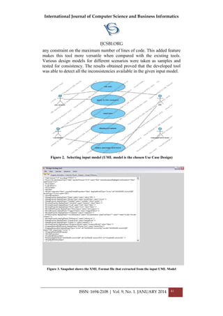

![International Journal of Computer Science and Business Informatics
IJCSBI.ORG
ISSN: 1694-2108 | Vol. 9, No. 1. JANUARY 2014 43
Figure 6 . Snapshot shows efficency of the given input design model
6. CONCLUSION AND FUTURE ENHANCEMENT
Inspection and testing of the software are the important approaches in
software engineering practice that addresses to reduce the amount of defects
in software products. Software inspection focuses on design specifications
in early phases of software development whereas traditional testing
approaches focus on implementation phases or later. Software inspection is
widely regarded as an effective defect finding technique. Recent research
has considered the application of tool support as a means to increase its
efficiency. During the design model, construction and validation of variety
of faults can be found. Testing at the early phase in software life cycle not
only increases quality but also reduces the cost incurred. The developed tool
can help to enforce the inspection process and provide support for finding
defects in the design model, and also compute the design efficiency on
deriving the error efficiency. This work would take care of the major
constraints imposed while creating design models such as class diagram, use
case diagram and sequence diagram. Further enhancement of the proposed
work is to address the other major constraints in class diagrams such as
inheritance, association, cardinality constraints and so on.
REFERENCES
[1] A.Egyed and D.S.Wile, Supporting for Managing Design-Time Decision, IEEE
Transactions on Software Engineering, 2006.
[2] A.Egyed, Fixing Inconsistencies in UML Design Models, ICSE, 2007.](https://image.slidesharecdn.com/vol9no1-january2014-171208072155/85/Vol-9-No-1-January-2014-46-320.jpg)
![International Journal of Computer Science and Business Informatics
IJCSBI.ORG
ISSN: 1694-2108 | Vol. 9, No. 1. JANUARY 2014 44
[3] A.Egyed, Instant Consistency Checking for UML, Proceedings of the International
Conference on Software Engineering, 2006.
[4] A.Egyed, E.Letier, A.Finkelstein, Generating and Evaluating Choices for Fixing
Inconsisentices in UML Design Models, International Conference on Software
Engineering, 2008.
[5] A Egyed, Automatically Detecting and Tracking Inconsistencies in Software Design
Models IEEE Transactions on Software Engineering, ISSN: 0098-5589, 2009.
[6] C.Nentwich, I.Capra and A.Finkelstein, xlinkit: a consistency checking and smart link
generation service, ACM transactions on Internet Technology, 2002.
[7] C.Nentwich, W. Emmerich and A.Finkelstein, Consistency Management with Repair
Actions, ICSE, 2003.
[8] Diana kalibatiene , Olegas Vasilecas , Ruta Dubauskaite , Ensuring Consistency in
Different IS models – UML case study , Baltic J.Modern Computing , Vol.1 , No.1-
2,pp.63-76 ,2013.
[9] Muhammad Usman, Aamer Nadeem, Tai-hoon Kim, Eun-suk Cho, A Survey of
Consistency Checking Techniques for UML Models , Advanced Software Engineering
& Its Applications,2008.
[10]R. Dubauskaite, O.Vasilecas, Method on specifying consistency rules among different
aspect models, expressed in UML, Elektronika ir elekrotechnika , ISSN 1392 -1215.
Vol.19, No.3, 2013.
[11]Rumbaugh, J., Jacobson, I., Booch, G., The Unified Modeling Language Reference
Manual. AddisonWesley, 1999.
[12] Amal Khalil and Juergen Dingel, Supporting the evolution of UML models in model
driven software developmeny: A Survey, Technical Report, School of Computing,
Queen’s University, Canada, Feb 2013.
This paper may be cited as:
Thirugnanam, M. and Subramaniam, S., 2014. An Efficient Design Tool to
Detect Inconsistencies in UML Design Models. International Journal of
Computer Science and Business Informatics, Vol. 9, No. 1, pp. 36-44.](https://image.slidesharecdn.com/vol9no1-january2014-171208072155/85/Vol-9-No-1-January-2014-47-320.jpg)
![International Journal of Computer Science and Business Informatics
IJCSBI.ORG
ISSN: 1694-2108 | Vol. 9, No. 1. JANUARY 2014 45
An Integrated Procedure for Resolving
Portfolio Optimization Problems using
Data Envelopment Analysis, Ant
Colony Optimization and Gene
Expression Programming
Chih-Ming Hsu
Minghsin University of Science and Technology
1 Hsin-Hsing Road, Hsin-Fong, Hsinchu 304, Taiwan, ROC
ABSTRACT
The portfolio optimization problem is an important issue in the field of investment/financial
decision-making and is currently receiving considerable attention from both researchers and
practitioners. In this study, an integrated procedure using data envelopment analysis (DEA),
ant colony optimization (ACO) for continuous domains and gene expression programming
(GEP) is proposed. The procedure is evaluated through a case study on investing in stocks
in the semiconductor sub-section of the Taiwan stock market. The potential average six-
month return on investment of 13.12% from November 1, 2007 to July 8, 2011 indicates
that the proposed procedure can be considered a feasible and effective tool for making
outstanding investment plans. Moreover, it is a strategy that can help investors make profits
even though the overall stock market suffers a loss. The present study can help an investor
to screen stocks with the most profitable potential rapidly and can automatically determine
the optimal investment proportion of each stock to minimize the investment risk while
satisfying the target return on investment set by an investor. Furthermore, this study fills the
scarcity of discussions about the timing for buying/selling stocks in the literature by
providing a set of transaction rules.
Keywords
Portfolio optimization, Data envelopment analysis, Ant colony optimization, Gene
expression programming.
1. INTRODUCTION
Portfolio optimization is a procedure that aims to find the optimal
percentage asset allocation for a finite set of assets, thus giving the highest
return for the least risk. It is an important issue in the field of
investment/financial decision-making and currently receiving considerable
attention from both researchers and practitioners. The first parametric model
applied to the portfolio optimization problem was proposed by Harry M.
Markowitz [1]. This is the Markowitz mean-variance model, which is the
foundation for modern portfolio theory. The non-negativity constraint
makes the standard Markowitz model NP-hard and inhibits an analytic](https://image.slidesharecdn.com/vol9no1-january2014-171208072155/85/Vol-9-No-1-January-2014-48-320.jpg)
![International Journal of Computer Science and Business Informatics
IJCSBI.ORG
ISSN: 1694-2108 | Vol. 9, No. 1. JANUARY 2014 46
solution. Although quadratic programming can be used to solve the problem
with a reasonably small number of different assets, it becomes much more
difficult if the number of assets is increased or if additional constraints, such
as cardinality constraints, bounding constraints or other real-world
requirements, are introduced.
Therefore, various approaches for tackling portfolio optimization problems
using heuristic techniques have been proposed. For example,
Anagnostopoulos and Mamanis [2] formulated the portfolio selection as a
tri-objective optimization problem that aims to simultaneously maximize the
expected return, as well as minimize risk and the number of assets held in
the portfolio. In addition, their proposed model also considered quantity
constraints and class constraints intended to limit the proportion of the
portfolio invested in assets with common characteristics and to avoid very
small holdings. The experimental results and a comparison revealed that
SPEA2 (strength Pareto evolutionary algorithm 2) [4] is the best algorithm
both for the constrained and unconstrained portfolio optimization problem,
while PESA (Pareto envelope-based selection algorithm) [3] is the runner-
up and the fastest approach of all models compared. Deng and Lin [5]
proposed an approach for resolving the cardinality constrained Markowitz
mean-variance portfolio optimization problem based on the ant colony
optimization (ACO) algorithm. Their proposed method was demonstrated
using test data from the Hang Seng 31, DAX 100, FTSE 100, S&P 100, and
Nikkei 225 indices from March 1992 to September 1997, which yielded
adequate results. Chen et al.[6]proposed a decision-making model of
dynamic portfolio optimization for adapting to the change of stock prices
based on time adapting genetic network programming (TA-GNP) to
generate portfolio investment advice. They determined the distribution of
initial capital to each brand in the portfolio, as well as to create trading rules
for buying and selling stocks on a regular basis, by using technical indices
and candlestick chart as judgment functions. The effectiveness and
efficiency of their proposed method was demonstrated by an experiment on
the Japanese stock market. The comparative results clarified that the TA-
GNP generates more profit than the traditional static GNP, genetic
algorithms (GAs), and the Buy & Hold method. Sun et al. [7] modified the
update equations of velocity and position of the particle in particle swarm
optimization (PSO) and proposed the drift particle swarm optimization
(DPSO) to resolve the multi-stage portfolio optimization (MSPO) problem
where transactions take place at discrete time points during the planning
horizon. The authors illustrated their approach by conducting experiments
on the problem with different numbers of stages in the planning horizon
using sample data collected from the S&P 100 index. The experimental
results and a comparison indicated that the DPSO heuristic can yield
superior efficient frontiers compared to PSO, GAs and two classical](https://image.slidesharecdn.com/vol9no1-january2014-171208072155/85/Vol-9-No-1-January-2014-49-320.jpg)
![International Journal of Computer Science and Business Informatics
IJCSBI.ORG
ISSN: 1694-2108 | Vol. 9, No. 1. JANUARY 2014 47
optimization solvers including LOQO and CPLEX. Woodside-Oriakhi et al.
[8] applied GAs, tabu search (TS) and simulated annealing (SA) to find the
efficient frontier in financial portfolio optimization that extends the
Markowitz mean-variance model to consider the discrete restrictions of buy-
in thresholds and cardinality constraints. The performance of their methods
was tested using publicly available data sets drawn from seven major market
indices. The implementation results indicated that the proposed methods
could yield better solutions than previous heuristics in the literature. Chang
and Shi [9] proposed a two-stage process for constructing a stock portfolio.
In the first stage, the investment satisfied capability index (ISCI) was used
to evaluate individual stock performance. In the second stage, a PSO
algorithm was applied to find the optimal allocation of capital investment
for each stock in the portfolio. The results of an experiment on investing in
the Taiwan stock market from 2005 to 2007 showed that the accumulated
returns on investment (ROIs) of the portfolios constructed by their proposed
approach were higher than the ROIs of the Taiwan Weighted Stock Index
(TWSI) portfolios. Sadjadi et al.[10] proposed a framework for formulating
and solving cardinality constrained portfolio problem with uncertain input
parameters. The problem formulation was based on the recent advancements
on robust optimization and was solved using GAs. Their proposed method
was examined on several well-known benchmark data sets including the
Hang Seng 31 (Hong Kong), DAX 100 (Germany), FTSE 100 (UK), S&P
100 (USA), and Nikkei 225 (Japan). The results indicated that D-norm
performs better than Lp-norm with relatively lower CPU time for the
proposed method. Yunusoglu and Selim [11] proposed a three-stage expert
system for stock evaluation and portfolio construction for a middle term
investment decision. The first stage eliminates the stocks that are not
preferred by investors. In the second stage, the acceptable stocks are scored
according to their performance by a fuzzy rule-based rating system. I the
final stage, the stocks contained in the resulting portfolio and their investing
weightings are determined through the mixed integer linear programming.
Their proposed system was validated by 61 stocks traded in Istanbul Stock
Exchange National-100 Index and the results indicated that the performance
of their approach was superior relative to the benchmark index in most of
the cases with different risk profiles and investment period lengths. Vercher
and Bermudez [12] presented a possibilistic model for a portfolio selection
problem where the uncertainty of the returns on a given portfolio was
modeled using LR-fuzzy numbers, including the expected return, downside
risk and skewness coefficient. A multi-objective evolutionary algorithm was
then used to select the efficient portfolios in the fuzzy risk–return tradeoff
with bound and cardinality constraints in order to meet the explicit
restrictions imposed by an investor. Demonstrating the proposed approach
with a dataset from the Spanish stock market yielded adequate results. Farzi](https://image.slidesharecdn.com/vol9no1-january2014-171208072155/85/Vol-9-No-1-January-2014-50-320.jpg)
![International Journal of Computer Science and Business Informatics
IJCSBI.ORG
ISSN: 1694-2108 | Vol. 9, No. 1. JANUARY 2014 48
et al. [13] proposed an approach for resolving the portfolio selection
problem based on quantum-behaved particle swarm optimization (QPSO).
The proposed QPSO model was employed to select the best portfolio in 50
supreme Tehran stock exchange companies with aims of optimizing the rate
of return, systematic and non-systematic risks, return skewness, liquidity
and sharp ratio. The comparison with traditional Markowitz’s and genetic
algorithms models revealed that the return of the portfolio obtained by the
QPSO was smaller than that in Markowitz’s classic model. However, the
QPSO can decrease risk and provide more versatile portfolios than the other
models.
The above-mentioned studies prove that soft computing techniques, such as
GAs, PSO and ACO, are an effective and efficient way to address portfolio
optimization problems. However, the concerns and interests of investors
need also to be considered. First, the total number of stocks that investors
can consider in their investment portfolio is usually extremely large.
Therefore, investors usually focus on a few stock components according to
their experience or principles for selecting stocks that have potential to
make profits. Second, most investors are interested in minimizing downside
risk since the return of stocks may not be normally distributed.
Unfortunately, the research on downside risk is relatively little compared to
the research that measures risk through the conventional variances used in
the traditional Markowitz mean-variance model. Third, investors usually
buy and sell their focused stocks several times during their investment
planning horizon. Here again, the research regarding the timing of
buying/selling stocks is scant.
2. PROBLEM FORMULATION
This study concentrates on the cardinality constrained portfolio optimization
problem, which is a variant of the Markowitz mean-variance model where
the portfolio can include at most c different assets. In addition, the minimum
proportion of the total investment of each asset contained in the portfolio is
also considered to reflect the fact that an investor usually sets a minimum
investment threshold for each asset held. Notably, the study measures the
variance (risk) of an asset by using the below-mean semi variance [14] to
reflect that only downside risk is relevant to an investor and assets
distributions may not be normally distributed. First, some notations are
defined, as follows:
N: the total number of assets available;
no: the total number of periods considered;
t
ir : the return of asset i in period t ( notNi ,...,2,1,,...,2,1 );
imr : the expected (mean) return of asset i ( Ni ,...,2,1 );
iw : the proportion of the total investment held in asset i ( Ni ,...,2,1 );](https://image.slidesharecdn.com/vol9no1-january2014-171208072155/85/Vol-9-No-1-January-2014-51-320.jpg)
![International Journal of Computer Science and Business Informatics
IJCSBI.ORG
ISSN: 1694-2108 | Vol. 9, No. 1. JANUARY 2014 49
ij : the correlation coefficient between assets i and j (
NjNi ,...,2,1,,...,2,1 );
*
r :the expected portfolio return;
c: the maximum number of assets in the portfolio;
minw : the minimum proportion of the total investment held in asset i, if any
investment is made in asset i ( Ni ,...,2,1 );
i : the decision variable that represents whether asset i ( Ni ,...,2,1 ) is held
in the portfolio ( 1i ) or not ( 0i ).
The below-mean semi variance for asset i can then be calculated as follows
[14]:
no
t
t
ii
m
i rmr
no
SV
1
2
)](,0max[
1
, Ni ,...,1 . (1)
Hence, the cardinality constrained portfolio optimization problem
considered in this study is formulated as shown below:
N
i
N
j
ij
m
j
m
iji SVSVww
1 1
Minimize (2)
subject to *
1
rmrw
N
i
ii
(3)
1
1
N
i
iw (4)
Niww iii ,...,2,1,min (5)
c
N
i
i 1
(6)
,...,N,ii 211,or0 . (7)
Eq. (2) intends to minimize the volatility (variance or risk) associated with
the portfolio. Eq. (3) ensures that the portfolio can yield an expected return
of *
r at least. Eq. (4) ensures that investment proportions sum to one while
a minimum investment threshold is considered to restrict asset investments
as shown in Eq. (5). Of particular importance is Eq. (5), which enforces that
the resulting proportion of iw is zero if asset i is not held in the portfolio,
i.e. 0i , and that the investment proportion of iw cannot be less than the
minimum proportion minw if asset i is held, i.e. 1i . Eq. (6) is the
cardinality constraint that ensures the total number of assets in the portfolio
does not exceed the maximum allowable number c. Finally, Eq. (7) is the
integrality constraint that reflects the inclusion or exclusion of an asset.](https://image.slidesharecdn.com/vol9no1-january2014-171208072155/85/Vol-9-No-1-January-2014-52-320.jpg)
![International Journal of Computer Science and Business Informatics
IJCSBI.ORG
ISSN: 1694-2108 | Vol. 9, No. 1. JANUARY 2014 50
3. METHODOLOGY ISSUES
3.1 Data Envelopment Analysis
Data envelopment analysis (DEA) is a method for measuring the relative
efficiencies of a set of similar decision making units (DMUs) through an
evaluation of their inputs and outputs. The two popular DEA models are the
CCR model developed by Charnes et al. [15] and the BCC model proposed
by Banker et al. [16]. In addition, DEA models can have an input or output
orientation. In this study, the objective of applying DEA to portfolio
optimization is to screen companies within a given industry on the basis of
their financial performance. Since the goal is to measure the underlying
financial strength of companies whose scale sizes may differ, the input-
oriented CCR model is more appropriate than the output-oriented BBC
model. Furthermore, it is easier to reduce the input quantities than to
increase the output quantities. Hence, the input-oriented CCR model is
applied here. Suppose the goal is to evaluate the efficiency of d independent
DMUs relative to each other based on their common m inputs and s outputs.
The input-oriented CCR model for evaluating the performance h0 of DMU0
can be formulated as follows:
m
i
ii
s
r
rr
xv
yu
h
1
0
1
0
0Maximize (8)
subject to dj
xv
yu
m
i
iji
s
r
rjr
,...,2,1,1
1
1
(9)
srur ,...,2,1,0 (10)
mivi ,...,2,1,0 (11)
where ijx ( 0 ) and rjy ( 0 ) represent the ith input and the rth output of
DMUj, respectively; and iv and ru denote the weight given to input i and
output r, respectively.
3.2 Ant Colony Optimization for Continuous Domains
Inspired by the foraging behavior of real ant colonies, Dorigo and his
colleagues in the early 1990’s were the first to introduce the ant colony
optimization (ACO) technique for the search of approximate solutions to
discrete optimization problems. While the original ACO algorithms were
designed to solve discrete problems, their adaptation to continuous
optimization problems has attracted much attention. Among these](https://image.slidesharecdn.com/vol9no1-january2014-171208072155/85/Vol-9-No-1-January-2014-53-320.jpg)
![International Journal of Computer Science and Business Informatics
IJCSBI.ORG
ISSN: 1694-2108 | Vol. 9, No. 1. JANUARY 2014 51
approaches, the ACO approach of Socha [17] is closest to the spirit of ACO
for discrete problems [18].
Suppose a population with cardinality of k is used to solve a continuous
optimization problem with n dimensions. The Gaussian function is usually
used as the probability density function (PDF) to estimate the distribution of
each member (ant) in the solution population. For the ith dimension, the jth
Gaussian function, with mean value i
j and standard deviation i
j , that is
derived from the jth member of the population with a cardinality of k, is
represented by:
2
2
2
)(
2
1
)(
i
j
i
jx
i
j
i
j exg
, ni ,...,1 ; kj ,...,1 ; x (12)
Hence, an ant can choose a value for dimension i by using a Gaussian
kernel, which is a weighted superposition of several Gaussian functions,
defined as:
k
j
i
jj
i
xgwxG
1
)()( , ni ,...,1 ; x (13)
where jw is the weight associated with the jth member of the population in
the mixture [18]. All solutions in the population are first ranked based on
their fitness with rank 1 for the best solution, and the associated weight of
the jth member of the population in the mixture is calculated by:
22
2
2
)1(
2
1 kq
r
j e
qk
w
, kj ,...,1 (14)
where r is the rank of the jth member and q( 0 ) is a parameter of the
algorithm[18]. Furthermore, each ant j must choose one of the Gaussian
functions ( 111
2
1
1 ,...,,...,, kj gggg ) for the first dimension [18], i.e. the first
construction step, with the probability:
k
l
l
j
j
w
w
p
1
, kj ,...,1 . (15)
Suppose the Gaussian function 1
*
j
g is chosen for the ant j in the first
dimension; the Gaussian functions 2
*
j
g to n
j
g * are then used for the
remaining n-1 construction steps. In addition, for the *
j th Gaussian function
in the ith dimension, the mean is set by:
i
j
i
j
x ** , ni ,...,1 , (16)
and the standard deviation is estimated by:](https://image.slidesharecdn.com/vol9no1-january2014-171208072155/85/Vol-9-No-1-January-2014-54-320.jpg)
![International Journal of Computer Science and Business Informatics
IJCSBI.ORG
ISSN: 1694-2108 | Vol. 9, No. 1. JANUARY 2014 52
k
j
i
j
i
j
i
j
xx
k 1
2
)(
1
** , ni ,...,1 (17)
where i
jx is the value of the ith decision variable in solution (ant)j and
)1,0( is the parameter that regulates the speed of convergence [18].
Once each ant has completed n construction steps, the worst s solutions in
the original population are replaced by the same number of best solutions
generated by the search process, thus forming a new solution population.
The search process is carried out iteratively until the stopping criteria are
satisfied and the near optimal solutions are obtained. The detailed execution
steps of the ant colony optimization for continuous domains, denoted by
ACO , are summarized as follows:
Step 1:Randomly or by using some principles, create an initial population
consisting of k solutions (ants) with n dimensions.
Step 2:Calculate the fitness of each solution and rank these solutions based
on their fitness with rank 1 for the best solution.
Step 3:For each solution j, choose one of the Gaussian functions (
11
2
1
1 ,...,, kggg ) for the first dimension, denoted by 1
*
j
g , based on the
probability obtained through Eqs. (14) and (15).
Step 4:For each solution j, generate a new solution by sampling the
Gaussian functions ),...,,( ***
21 n
jjj
ggg whose means and standard
deviations are calculated using Eqs. (16) and (17).
Step 5:Replace the worst s solutions in the original population by the same
number of the best solutions generated in Step 4, thus forming a new
solution population.
Step 6:If the termination criteria are satisfied, stop the search process and
obtain the near optimal solutions. Otherwise, execute Steps 2 to 5
iteratively.
3.3 Gene Expression Programming
Gene expression programming (GEP) first developed by Ferreira [19] is an
evolutionary methodology, based on the principles of Darwinian natural
selection and biologically inspired operations, to evolve populations of
computer programs in order to solve a user-defined problem. In GEP, the
genes consist of a head containing symbols to represent both functions
(elements from the function set F) and terminals (elements from the
terminal set T), and a tail containing only terminals. Suppose, for a problem,
the number of arguments in the function with the most arguments is and
the length of the head is h. Then, the length of the tail t is evaluated by the
equation:
1)1( ht . (18)](https://image.slidesharecdn.com/vol9no1-january2014-171208072155/85/Vol-9-No-1-January-2014-55-320.jpg)
![International Journal of Computer Science and Business Informatics
IJCSBI.ORG
ISSN: 1694-2108 | Vol. 9, No. 1. JANUARY 2014 53
As an example, consider a gene composed of [Q, ×, ÷, -, +, a, b] where the
number of arguments in the function with the most arguments is 2. If the
length of the head h is set as 10, the length of the tail t can be obtained as
11, i.e. 1)12(10 , and the length of the gene is 21, i.e. 1110 . One such
gene is illustrated as follows:
bbaaababbabQababQ
098765432109876543210
(19)
where the tail is shown in bold and “Q” represents the square root function.
The above gene (genotype) can be represented by an expression tree
(phenotype) as shown in Figure 1 and decoded as follows:
][ babab . (20)
The general execution steps of GEP are presented by Ferreira[19], and are
briefly summarized as follows:
Step 1: Randomly generate an initial population of chromosomes.
Step 2: Express the chromosomes and evaluate the fitness of each
individual.
Step 3: Select chromosomes from the population using a random probability
based on the fitness and replicate the selected chromosomes.
Step 4: Randomly apply genetic operators to the replicated chromosomes in
Step 3, thus creating the next generation. The genetic operators
include mutation, IS (insertion sequence) transposition, RIS (root
insertion sequence) transposition, gene transposition, one-point
recombination, two-point recombination and gene recombination.
Step 5: When the termination criterion is satisfied, the outcome is
designated as the final result of the run. Otherwise, Steps 2 to 4 are
executed iteratively.
Figure 1. An example of the expression tree in GEP
4. PROPOSED PORTFOLIO OPTIMIZATION PROCEDURE
The proposed optimization procedure comprising three stages is described
in the following sub-sections.
4.1 Selection of Stocks
In the first stage, the DEA technique is used to select stocks with the most
potential for making profits. First, four financial variables including total](https://image.slidesharecdn.com/vol9no1-january2014-171208072155/85/Vol-9-No-1-January-2014-56-320.jpg)
![International Journal of Computer Science and Business Informatics
IJCSBI.ORG
ISSN: 1694-2108 | Vol. 9, No. 1. JANUARY 2014 54
assets, total equity, cost of sales and operating expenses are defined as
inputs in the DEA model and two variables including net sales and net
income are defined as outputs. This is in line with previous studies [20–22].
Next, the input-oriented CCR model is applied to evaluate the underlying
fundamental financial strength of companies (DMUs) by using the financial
data collected from the financial reports, which consists of the four inputs
and two outputs. The companies are then ranked based on their efficiency
scores with the highest score as rank 1. In addition, the companies with the
same efficiency score are further ranked based on their earnings per share
(EPS) in a descending order. Hence, companies with rank 1, up to and
including c, are then selected as the essential candidate companies (stocks)
in the investment portfolio. These are the maximum allowable number of
assets in the portfolio, as shown in Eq. (6).
4.2 Optimization of a Portfolio
In the second stage, the ACO algorithm is applied to select the final stocks
in the investment portfolio, as well as optimize the investment proportion of
each selected stock. First, the expected weekly return of stock i, i.e. imr in
Eq. (3), the below-mean semi variance for stock i, i.e. m
iSV in Eq. (2), and
the correlation coefficient between stocks i and j, i.e. ij in Eq. (2), are
calculated based on the weekly trading data in the stock market. Next, the
ACO algorithm presented in Section 3.2 is used to resolve the cardinality
constrained portfolio optimization problem as formulated in Eqs. (2) to (7).
Since the number of companies with superior financial strength included in
the previous stage exactly equals c, the cardinality constraint in Eq. (6) is
fulfilled. In addition, the constraint regarding the expected return in Eq. (3)
is designed into the objective function in Eq. (2). Hence, the objective
function to be minimized in ACO is defined as follows:
}0,Max{
1
*
1 1
ACO
N
i
ii
N
i
N
j
ij
m
j
m
iji mrwrMSVSVwwf (21)
where M is a very large number that represents the penalty, while the
portfolio cannot yield an expected return better than the desired level *
r as
shown in Eq. (3). In addition, the obtained jth solution ),...,,( 21 c
jjj xxx , i.e. the
jth ant in the solution population with a cardinality of k, from ACO is
modified according to the following equation:
kjci
wxx
y
i
j
i
ji
j ,...,1,,...,2,1,
otherwise0
if min
. (22)
Therefore, the jth solution ( kj ,...,1 ) in ACO can now be transformed
into a feasible solution for the cardinality constrained portfolio optimization
problem. The transformation is based on the following equation:](https://image.slidesharecdn.com/vol9no1-january2014-171208072155/85/Vol-9-No-1-January-2014-57-320.jpg)
![International Journal of Computer Science and Business Informatics
IJCSBI.ORG
ISSN: 1694-2108 | Vol. 9, No. 1. JANUARY 2014 55
ci
y
y
w c
i
i
j
i
j
i ,...,2,1,
1
. (23)
In this manner, all iw s lie between minw and 1, and the sum of iw s in each
solution equals one, i.e.
c
i
iw
1
1; thus the constraints in Eqs. (4), (5) and (7)
are met.
4.3 Buying/Selling of Stocks
In the last stage, the GEP technique is utilized to forecast stock closing
prices and transaction rules are designed to determine the optimal timing for
buying/selling stocks. First, fifteen technical indicators including (1) 10-day
moving average, (2) 20-day bias, (3) moving average
convergence/divergence, (4) 9-day stochastic indicator K, (5)9-day
stochastic indicator D, (6) 9-day Williams overbought/oversold index, (7)
10-day rate of change, (8) 5-day relative strength index, (9) 24-day
commodity channel index, (10) 26-day volume ratio, (11) 13-day
psychological line, (12) 14-day plus directional indicator, (13)14-day minus
directional indicator, (14) 26-day buying/selling momentum indicator and
(15)26-day buying/selling willingness indicator are calculated based on the
historical stock trading data. These indicators will serve as the input
variables of GEP forecasting models, which is in line with previous studies
[23–28].The technical indicators on the last trading day of each week, along
with the closing price on the last trading day of the following week, are then
randomly partitioned into training and test data based on a pre-specified
proportion, e.g., 4:1. Next, the GEP algorithm is utilized to construct several
forecasting models and an optimal forecasting model is determined based on
simultaneously minimizing the root mean squared errors (RMSEs) of the
training and test data, named ModelGEP. Let ip represent the closing price
on the last trading day of the current week and let ipˆ represent the
forecasted closing price on the last trading day of the next week for stock i.
Four transaction rules can then be designed as follows:
(1) IF (Stock i is held) AND ( pp ˆ ), THEN (Do not take any action);
(2) IF (Stock i is held) AND ( pp ˆ ), THEN (Sell stock i on the next
trading day);
(3) IF (Stock i is not held) AND ( pp ˆ ), THEN (Buy stock i on the next
trading day);
(4) IF (Stock i is not held) AND ( pp ˆ ), THEN (Do not take any action).
Using these rules and the forecasted closing stock price obtained by the
ModelGEP, an investor can make buy/sell decisions for each stock on the last
trading day of each week of the investor’s planning horizon.](https://image.slidesharecdn.com/vol9no1-january2014-171208072155/85/Vol-9-No-1-January-2014-58-320.jpg)
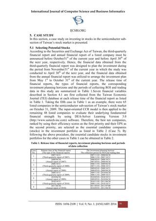
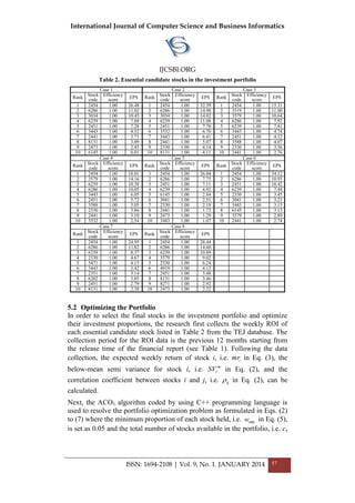
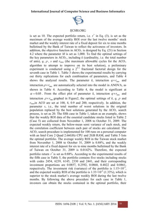
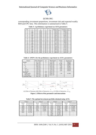
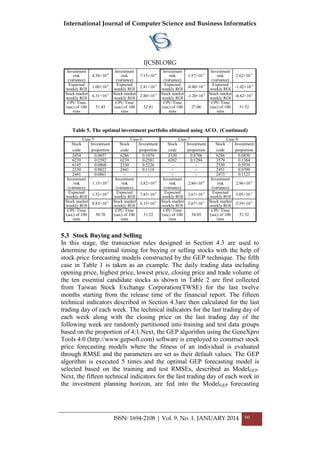
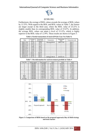
![International Journal of Computer Science and Business Informatics
IJCSBI.ORG
ISSN: 1694-2108 | Vol. 9, No. 1. JANUARY 2014 63
6. CONCLUSIONS
In this study, the data envelopment analysis (DEA), ant colony optimization
for continuous domains (ACO ) and gene expression programming (GEP)
are utilized to develop an integrated approach to deal with the portfolio
optimization problems. The feasibility and effectiveness of the proposed
procedure are verified through a case study on investing stocks in the
semiconductor sub-section of Taiwan stock market over the period from
November1, 2007 to July8, 2011. The obtained results show that the
average return on investment (ROI) of six months can attain a very high
level of 13.12%, as well as the ROI value for the worst case is still higher
than the normal yearly interest rate of a fixed deposit for six to nine months
in Taiwan. Next, the experimental results indicates that the third stage of the
proposed portfolio optimization procedure indeed functions to assist the
investors for determining the optimal timing for buying/selling stocks thus
avoiding a substantial investment loss and eventually making a superior
profit. Furthermore, the proposed procedure can positively assist the
investors to make profits even though the overall stock market suffers a loss.
The present study makes four main contributions to the literature. First, it
successfully proposes a systematic procedure for portfolio optimization
using based on DEA, ACOR and GEP based on the data collected from the
financial reports and stock markets. Second, it can help an investor to screen
stocks with the most profitable potential rapidly, even when he or she lacks
sufficient financial knowledge. Third, it can automatically determine the
optimal investment proportion of each stock to minimize the investment risk
while satisfying the target return on investment set by an investor. Fourth, it
can fill the scarcity of discussions about the timing for buying/selling stocks
in the literature by providing a set of transaction rules based on the actual
and forecasted stock prices.
REFERENCES
[1] Markowitz, H.M.Portfolio selection.J. Finance, 7, 1 (1952), 77–91.
[2] Anagnostopoulos, K.P.,and Mamanis, G. A portfolio optimization model with three
objectives and discrete variables.Comput. Oper. Res., 37, 7 (2010), 1285–1297.
[3] Zitzler, E., Laumanns, M., and Thiele, L. SPEA2: Improving the Strength Pareto
Evolutionary Algorithm. Computer Engineering and Networks Laboratory (TIK),
Department of Electrical Engineering, Swiss Federal Institute of Technology (ETH),
Zurich, Switzerland, 2001.
[4] Corne, D. W., Knowles, J. D., and Oates, M. J. The Pareto envelop-based selection
algorithm for multiobjective optimization.InProceedings of the 6th International
Conference on Parallel Problem Solving from Nature(Paris, France, September 18–20,
2000). Springer-Verlag, Heidelberg, Berlin, 2000, 839–848.
[5] Deng, G. F., and Lin, W. T. Ant colony optimization for Markowitz mean-variance
portfolio model. In Panigrahi, B. K., Das, S., Suganthan, P.N., and Dash, S. S. (Eds.),](https://image.slidesharecdn.com/vol9no1-january2014-171208072155/85/Vol-9-No-1-January-2014-66-320.jpg)
![International Journal of Computer Science and Business Informatics
IJCSBI.ORG
ISSN: 1694-2108 | Vol. 9, No. 1. JANUARY 2014 64
Swarm, Evolutionary, and Memetic Computing. Springer-Verlag, Heidelberg, Berlin,
2010, 238–245.
[6] Chen, Y., Mabu, S., and Hirasawa, K. A model of portfolio optimization using time
adapting genetic network programming.Comput. Oper. Res., 37, 10 (2010), 1697–
1707.
[7] Sun, J., Fang, W., Wu, X.J., Lai, C.H., and Xu, W.B.Solving the multi-stage portfolio
optimization problem with a novel particle swarm optimization.Expert Syst. Appl., 38,6
(2011), 6727–6735.
[8] Woodside-Oriakhi, M., Lucas, C., and Beasley, J.E.Heuristic algorithms for the
cardinality constrained efficient frontier.Eur. J. Oper. Res., 213, 3 (2011), 538–550.
[9] Chang, J.F., and Shi, P. Using investment satisfaction capability index based particle
swarm optimization to construct a stock portfolio. Inf. Sci., 181, 14 (2011), 2989–2999.
[10]Sadjadi, S. J., Gharakhani, M., and Safari, E. Robust optimization framework for
cardinality constrained portfolio problem. Appl. Soft Comput., 12, 1 (2012), 91–99.
[11]Yunusoglu, M. G., and Selim, H. A fuzzy rule based expert system for stock evaluation
and portfolio construction: an application to Istanbul Stock Exchange. Expert Syst.
Appl., 40, 3(2013), 908–920.
[12]Vercher, E., and Bermudez, J. D. A possibilistic mean-downside risk-skewness model
for efficient portfolio selection. IEEE. T. Fuzzy Syst., 21,3 (2013), 585–595.
[13]Farzi, S., Shavazi, A. R., and Pandari, A. Using quantum-behaved particle swarm
optimization for portfolio selection problem. Int. Arab J. Inf. Technol., 10, 2 (2013),
111–119.
[14]Markowitz, H.M.Portfolio Selection. John Wiley and Sons, New York, 1959.
[15]Charnes, A., Cooper, W. W., and Rhodes, E. Measuring the efficiency of decision
making units.Eur. J. Oper. Res., 2, 6 (1978), 429–444.
[16]Banker, R.D., Charnes, A., and Cooper, W. W. Some models for estimating technical
and scale inefficiencies in data envelopment analysis.Manage. Sci. 30, 9 (1984), 1078–
1092.
[17]Socha, K. ACO for continuous and mixed-variable optimization.In Dorigo, M.,
Birattari, M., Blum, C., Gambardella, L.M., Mondada, F., and Stutzel, T. (Eds.), Ant
Colony Optimization and Swarm Intelligence. Springer, Brussels, Belgium, 2004, 25–
36.
[18]Blum, C. Ant colony optimization: introduction and recent trends.Phys. Life Rev., 2, 4
(2005), 353–373.
[19]Ferreira, C. Gene expression programming: a new adaptive algorithm for solving
problems.Complex Syst., 13, 2 (2001), 87–129.
[20]Chen, Y. S., and Chen, B. Y. Applying DEA, MPI, and grey model to explore the
operation performance of the Taiwanese wafer fabrication industry. Technol.
Forecasting Social Change, 78, 3 (2011), 536–546.
[21]Lo, S. F., and Lu, W. M. An integrated performance evaluation of financial holding
companies in Taiwan. Eur. J. Oper. Res., 198, 1 (2009), 341–350.
[22]Chen, H. H. Stock selection using data envelopment analysis. Ind. Manage. Data Syst.,
108, 9 (2008), 1255–1268.
[23]Chang, P.C., and Liu, C.H.A TSK type fuzzy rule based system for stock price
prediction. Expert Syst. Appl., 34, 1 (2008), 135–144.](https://image.slidesharecdn.com/vol9no1-january2014-171208072155/85/Vol-9-No-1-January-2014-67-320.jpg)
![International Journal of Computer Science and Business Informatics
IJCSBI.ORG
ISSN: 1694-2108 | Vol. 9, No. 1. JANUARY 2014 65
[24]Huang, C.L., and Tsai, C.Y.A hybrid SOFM-SVR with a filter-based feature selection
for stock market forecasting. Expert Syst. Appl., 36, 2 (2009), 1529–1539.
[25]Ince, H., and Trafalis, T. B. Short term forecasting with support vector machines and
application to stock price prediction. Int. J. Gen. Syst., 37, 6 (2008), 677–687.
[26]Kim, K.J., and Han, I. Genetic algorithms approach to feature discretization in artificial
neural networks for the prediction of stock price index.Expert Syst. Appl., 19, 2 (2000),
125–132.
[27]Kim, K.J., and Lee, W.B.Stock market prediction using artificial neural networks with
optimal feature transformation.Neural Compu. Appl., 13, 3 (2004), 255–260.
[28]Tsang, P.M., Kwok, P., Choy, S.O., Kwan, R., Ng, S.C., Mak, J., Tsang, J., Koong, K.,
and Wong,T.L. Design and implementation of NN5 for Hong Kong stock price
forecasting.Eng. Appl. Artif. Intell., 20, 4 (2007), 453–461.
This paper may be cited as:
Hsu, C. M., 2014. An Integrated Procedure for Resolving Portfolio
Optimization Problems using Data Envelopment Analysis, Ant Colony
Optimization and Gene Expression Programming. International Journal of
Computer Science and Business Informatics, Vol. 9, No. 1, pp. 45-65.](https://image.slidesharecdn.com/vol9no1-january2014-171208072155/85/Vol-9-No-1-January-2014-68-320.jpg)
![International Journal of Computer Science and Business Informatics
IJCSBI.ORG
ISSN: 1694-2108 | Vol. 9, No. 1. JANUARY 2014 66
Emerging Technologies:
LTE vs. WiMAX
Mohammad Arifin Rahman Khan
Lecturer, Department of CSE
Bangladesh University
Dhaka, Bangladesh
Md. Sadiq Iqbal
Assistant professor, Department of CSE,
Bangladesh University
Dhaka, Bangladesh
ABSTRACT
There are two up-and-coming technologies and these two are the 3GPP LTE whose
complete meaning is Third Generation Partnership Project Long Term Evolution and the
IEEE 802.16 WiMAX whose full meaning is Worldwide Interoperability for Microwave
Access. The main aspire found from both technologies are to give mobile data transmission,
voice communication and video services by promoting sound level cost deployment and
service models through friendly architectures for Internet and protocols. It is as well as true
that, that are being well thought-out like a candidate for the Fourth Generation (4G) of
Mobile Communications or networks. However, the analyses from the case study of this
paper is performing a depth assessment between the LTE and WiMAX standards and
delves into the intricacies study with each of them.
Keywords
Long Term Evolution, Worldwide Interoperability for Microwave Access, Circuit Switched
(CS), Radio Access Network, Orthogonal Frequency Division Multiple Access, Quality of
Service.
1. INTRODUCTION
It is true that the telecommunication user is continuously growing up.
However, the first generation of wireless communication has followed by
the analog technology and has been replaced by the technique of digital
system. The telecommunication network of the second generation started
with a circuit-switched (CS) approach called the Global System for Mobile
Communication (GSM) [1]. From the technology guide, it is obvious that,
circuit-switched approach was well known Fixed Telephone System and as
well as got permission the compatibility of both systems. Without a doubt it
is understandable for everyone that, internet facility makes the mobile
communication more global. Again, General Packet Radio Service has
shown his own performance in the area of mobile communication when the
plan of bringing data transmission to the devices of mobile, lead to the
first packet-switching extension of Global System for Mobile](https://image.slidesharecdn.com/vol9no1-january2014-171208072155/85/Vol-9-No-1-January-2014-69-320.jpg)
![International Journal of Computer Science and Business Informatics
IJCSBI.ORG
ISSN: 1694-2108 | Vol. 9, No. 1. JANUARY 2014 67
communication. Furthermore, the unbroken growth of mobile users guides
to several GSM extensions and finally leads to Universal Mobile
Telecommunications System which was standardized by the Third
Generation Partnership Project. From the technological history it has cleared
to each person that, Third Generation has guided by the UMTS and it has
made the deployment more difficult with cost-intensive because Universal
Mobile Telecommunication System required new frequency and base
station. Alternatively, Telecommunication sector has given huge data rate
support for their client [1].
Moreover, from technological development, it has found that, the Fourth
Generation (4G) of mobile technology does not maintain any circuit-
switched domain. On the other hand it has found from a deep analysis result
that, the mobile user has grown dramatically and therefore, it has needed
more and more data transfer which shows that efficiencies and more
advanced mobile networks are needed [2]. It is also observable result that,
the mobile handset has continuously developed from plain phones to general
purpose computers which is called Smartphone is a key driver for the fourth
generation networks. From the smart phone, the mobile user has got further
mobile services that go beyond telephony and messaging. Particularly fresh
examine a scenario like Mobile Payment, IPTV or Real-time gaming has
need of very low delay, high bandwidth and also high availability [3]. In
addition to the communication networks of fourth generation can be used to
carry high speed access to more rural area’s which are not enclosed by the
help of fixed high speed networks. International Telecommunication Union
Radio and the Communication Sector have mentioned the International
Mobile Telecommunications Advanced specified the necessity for fourth
generation network standards. However, in the term of Fourth Generation
(4G) networks is broadly used for highly developed telecommunication
networks based on Orthogonal Frequency Division Multiple Access
(OFDMA), use Multiple Input Multiple Output (MIMO) and have an IP-
only architecture.
However, this paper will clearly present the two most ordinary approaches
for the next generation telecommunication networks that are Long Term
Evolution (LTE) and Worldwide Interoperability for Microwave Access
(WiMAX). The key explanation of protocol architecture and characteristics
for LTE and WiMAX will be discussed broadly in the Section of Protocols,
Hardware Configurations and Multimedia and from those section everyone
will be understand clearly the main difference for both of technologies in
various aspects such as hardware with Network scenarios and Multimedia.
From the part of Future Developments, it will be analysis briefly for the
comparison future development of LTE and WiMAX. Furthermore,](https://image.slidesharecdn.com/vol9no1-january2014-171208072155/85/Vol-9-No-1-January-2014-70-320.jpg)
![International Journal of Computer Science and Business Informatics
IJCSBI.ORG
ISSN: 1694-2108 | Vol. 9, No. 1. JANUARY 2014 68
summarizes for this paper will be publish from the last section in
conclusion.
2. PROTOCOLS
Networking protocols helps to establish the data communication between
the sender and receiver. However, it is very important to understand the type
of protocol because the Packet switching performance depends on the
quality and the structure of protocol.
2.1 WiMAX Protocol Architecture
The WiMAX communication system is an end-to-end, all-IP wireless
system designed to provide wide area mobile access to broadband IP
services. 802.16 employs the Open system interconnect OSI physical (PHY)
and media access control (MAC) layer to reference the air interface and the
wireless medium. The purpose of the Physical layer is the transport of data.
The PHY uses the following techniques to ensure efficient Delivery of data
[4]. They include OFDM, TDD, and FDD and Adaptive Antenna systems.
Table 1: Provides key physicals layer attributes of the Mobile WiMAX Parameters [5]
Duplex Primarily TDD
Channel Bandwidth From 1.25MHz to 10mhz
Modulation type QPSK, 16QAM,64QAM (down-link only)
Multiple Access Technique OFDMA
TDMA frame duration 5ms
Number of symbols per frame 48
Sub-carrier spacing 10.94 kHz
Symbol duration 102.9 us
Typical cyclic prefix 1/8 symbol period
Multipath migration OFDM/Cyclic prefix
Base station synchronization Frequency and time synchronization
required
Forward error correction Convolution is coding at rates1/2,2/4,3/4
and 5/6 and repetition coding at rates /2,1/3
and 1/6
Advanced antenna techniques Space time coding and spatial multiplexing
The MAC layer provides intelligence for the PHY layer by utilizing the
MAC protocol data units PDU to exchange information between the Base
Station and Subscriber Station. The WiMAX protocol stack also includes
sub- layers [6] and the functional purposes include:
The MAC privacy sub-layer, where most authentication, encryption and key
exchange for traffic encryption is handled, MAC sub-layer, where framing,](https://image.slidesharecdn.com/vol9no1-january2014-171208072155/85/Vol-9-No-1-January-2014-71-320.jpg)
![International Journal of Computer Science and Business Informatics
IJCSBI.ORG
ISSN: 1694-2108 | Vol. 9, No. 1. JANUARY 2014 69
packing error handling and quality of services are supported, MAC
convergence sub-layer, where an upper layer packet can be encapsulated for
transmission, Below is simplified illustration of IP - based WiMAX network
architecture [7]. All over the network can be divided by logically into the
following parts such as, Mobile Stations (MS) which is used from the last
part of user to right to use the network and the Base Station (BS) which is in
charge for given that the air interface to the MS. There are some
supplementary functions that may be part of the BS are micro mobility
management functions, for example, session management, multicast group
management, Dynamic Host Control Protocol (DHCH proxy), key
administration, handoff triggering and tunnel establishment, RRM whose
full meaning is Radio Resource Management, Quality of Service policy
enforcement also the traffic classification. ASN which means Access
Service Network, gateway generally acts as a layer two traffic aggregation
point within an Access Service Network. Supplementary functions include
the resource of radio management and admission control, caching of
subscriber profiles and encryption keys, the functionality of AAA Client,
CSN means Connectivity service network, which provides Internet Protocol
connectivity and all the Internet Protocol center network functions [8]. The
connectivity services network (CSN) similar to the UTRAN is used as a link
between the core network CN and the user equipment UE. Moreover, it is
also true that, the IP address Management is also maintains by the CSN.
Figure 1: IP-Based WiMAX Network Architecture](https://image.slidesharecdn.com/vol9no1-january2014-171208072155/85/Vol-9-No-1-January-2014-72-320.jpg)
![International Journal of Computer Science and Business Informatics
IJCSBI.ORG
ISSN: 1694-2108 | Vol. 9, No. 1. JANUARY 2014 70
2.2 LTE Protocol Structure
Table 2: Provides key physicals layer attributes of the Mobile LTE Parameters [10]
Duplex FDD and TDD
Channel Bandwidth From 1.25mhz to 20mhz
Modulation type QPSK,16QAM,64QAM (optional in UL)
Multiple Access Technique Downlink: OFDMA,
Uplink :SCFDMA
TDMA frame duration 10ms with 1 ms sub-frame
Number of symbols per frame 140
Sub-carrier spacing 15 kHz
Symbol duration 66.7 us
Typical cyclic prefix 4.69 and 16.67 us
Multipath migration OFDM/Cyclic prefix
Base station synchronization Frequency and time synchronization required
Forward error correction 1/3 rate Convolution and turbo coding
Advanced antenna techniques MIMO 2X2, 4X4
In general it is found from the 3GPP specifications for Long Term
Evaluation that the communication network of radio access is mainly
divided split two separate parts, the first one is E-UTRA whose full
meaning is the Evolved UMTS Terrestrial Radio Access and the another one
is E-UTRAN whose complete meaning is the Evolved UMTS Terrestrial
Radio Access Network [9]. Again, the Mobile part of LTE describes by the
E-UTRA and on the other hand E-UTRAN who explains the BS part and the
eNB sector has described by that explanation.
Again, from the side of LTE qualifications, 3GPP is running on a
complementary task called the SAE whose full meaning is System
Architecture Evolution and it is defines the split between EPC and LTE.
This new architecture is a flatterer, packet - only center network that will
assist deliver the highest throughput, lower latency and lower cost with the
purpose of LTE [12]. EPC component's description and is realized through
the following elements:
Serving Gateway (SG-W) - The main job for SGW is like a part of a data
plane whose major function is to manage the client for example, plane
mobility and be acting as a demarcation point between the core networks
and RAN. Again, SGW controls data paths between the PDN Gateway and
the eNodeBs. From a functional point of view, the SGW is shows like an](https://image.slidesharecdn.com/vol9no1-january2014-171208072155/85/Vol-9-No-1-January-2014-73-320.jpg)
![International Journal of Computer Science and Business Informatics
IJCSBI.ORG
ISSN: 1694-2108 | Vol. 9, No. 1. JANUARY 2014 71
extinction position of the data frame communication network crossing point
towards E-UTRAN [13][21]. Gateway (PGW) PDN – such as the SGW, the
PDN Gateway is the execution position of the packet data crossing point
towards the Packet Data Networks [21]. Like a great secure position when it
is thinking for sessions towards the outside Packet Data Networks, PDN
Gateway supports the MME whose full meaning is Mobility Management
Entity. However, from the function of Mobility Management Entity, it is
clear to understand that, he is doing like a jointing component with the
Exact Perform the signaling and controlling. This shows the exact perform
the signaling and control function to manage the UE access to network
connections. Mobility Management Entity maintains all control plane
functions related to client and the session management. Moreover, a lot of
eNode elements is maintains by the Mobility Management Entity (MME).
Figure 2: 3GPP LTE Network Architecture
3. HARDWARE CONFIGURATION
3.1 WiMAX Base station
In WIMAX, the base station has a connection with the public network
which utilizes optic fibers, cables, microwave links or any other point to
point connections offering a high speed. The base station feeds the customer
premises equipment (CPE) also known as the subscriber station by the use
of a non- line of sight or a line of sight point to multipoint connectivity. The
limitation in a worldwide acceptance of the broadband wireless access has
been as a result of the customer premises equipment (CPE).](https://image.slidesharecdn.com/vol9no1-january2014-171208072155/85/Vol-9-No-1-January-2014-74-320.jpg)
![International Journal of Computer Science and Business Informatics
IJCSBI.ORG
ISSN: 1694-2108 | Vol. 9, No. 1. JANUARY 2014 72
Figure 3: WiMAX Base Station and network backbone [14]
The base station for WiMAX is typically made of a tower and an indoor
electronics. In the theory WiMAX base station can cover up to a 50km
radius or 30miles while in practice it is only limited to 10km or 6miles.
Within the coverage distance of the base station, any node can be able to
have internet reception [15]. There is the allocation of uplink and downlink
bandwidth to its subscribers based on their need by the use of the MAC
layer in the standard. It is needed to justify the Components of WiMAX
Base Stations’ Hardware Structure and the hardware structure consists of
four parts:
Ethernet Switch Fabric: This helps to achieve system expansibility
by offering help to multi MAC line cards access through Giga
Ethernet.
Multi PHY Channel Cards: The card facilitate in the
QPSK/16QAM/64QAM modulation and demodulation. Also the
card has an RF front end module that performs RF signal
transceiver.
FPGA: This instigates the interface conversions between DS1 and
SP13, package router.
MAC line card; It has a maximum throughput of about 100Mbps and
it maintain up to four PHY channel card. The MAC line card centers
on Intel IKP2350 to implement WiMAX and IPV4 routing
Encrypt/Decrypt, Ethernet IPV4 forwarding.](https://image.slidesharecdn.com/vol9no1-january2014-171208072155/85/Vol-9-No-1-January-2014-75-320.jpg)
![International Journal of Computer Science and Business Informatics
IJCSBI.ORG
ISSN: 1694-2108 | Vol. 9, No. 1. JANUARY 2014 73
Figure 4: WiMAX Base Station hardware structures [14]
The Intel2350 help WiMAX MAC to carry out a high data throughput and
very scalable architecture to meet different standard options and service
requirements.
3.2 LTE Hardware
The hardware components making up the Long Term Evolution (LTE) are
the base stations, antennas, and feeders. The base station of an LTE is called
an eNodeB. This eNodeB is the major aspect of an LTE RAN (Radio
Access Network) structural design. To plan a network deployment for LTE
the operator takes some factors into consideration which includes,
determining if the existing cell site can support the new equipment. The
issue of antenna size for the new installation has to be considered. It should
be understood that LTE leverages Multiple In, Multiple Out (MIMO) which
control group of antenna at the base station. Also the distance of the cell site
to the wire line infrastructure is to be considered and the cell site can
leverage fiber for backhaul if it is located less than one mile. This is a good
practice for transporting LTE traffic.
3.3 Comparison of WiMAX and LTE Hardware
The technologies of both WiMAX and LTE are somewhat different but both
of them share the same methodology for downlinks. The two have Multiple
Input Multiple Output (MIMO) which means that two or more antennas are
used to receive information from a single cell site to expand reception. Also
both WiMAX and LTE use the downlink from the cell tower to the end user
which is enhanced with the Orthogonal Frequency Division Multiplexing
(OFDM) which allows video and multimedia transmission [15].](https://image.slidesharecdn.com/vol9no1-january2014-171208072155/85/Vol-9-No-1-January-2014-76-320.jpg)
![International Journal of Computer Science and Business Informatics
IJCSBI.ORG
ISSN: 1694-2108 | Vol. 9, No. 1. JANUARY 2014 74
4. MULTIMEDIA – WiMAX vs. LTE
In terms of mobile multimedia WiMAX and LTE systems can be used to
complement each other. LTE offers coverage over large areas and unlimited
roaming whist WiMAX offers high speed data rates offering mobile
broadband in hotspot areas [16].
4.1 Mobile Multimedia and standards
Mobile multimedia consisted almost entirely of devices that become mobile
by virtue of the cellular networks i.e. LTE/3G type networks. The
requirements for these devices have been defined by the third generation
partnership projects (3GPP and 3GPP2); thus devices used are called 3GPP
devices. An example of mobile TV technology standards, such as DVB-H,
DMB has emerged, which have aligned themselves closely to the 3GPP
standards.
However, it is possible with a WiMAX network to accommodate a range of
new devices and services that work on technologies such as Multicast
Streaming, IPTV, VoIP, Broadband Data and Multimedia downloads.
Because Interworking is an important part of a WiMAX network,
LTE/3GPP specifications are an important design consideration for
applications in WiMAX networks [17]. Example of a Multimedia device
working in a multiple standard environment as previously mentioned, if we
look at a case of a WiMAX mobile phone. It could say this phone should
have the ability to work under a Wi-Fi, CDMA, 3G-UMTS or GSM. So in
order to use this phone the manufacture will have to make sure it will
operate under the IEEE 802.16e Standard as well as to use the GSM forum
3GPP (2) standards and comply with OMA rules for encryption. Other
standards such as DVB-H would also have to be considered. An example of
this challenging standardization issue can be seen in Figure 5.
Figure 5: Example of standardization issues Concerning LTE and Wimax systems](https://image.slidesharecdn.com/vol9no1-january2014-171208072155/85/Vol-9-No-1-January-2014-77-320.jpg)
![International Journal of Computer Science and Business Informatics
IJCSBI.ORG
ISSN: 1694-2108 | Vol. 9, No. 1. JANUARY 2014 75
4.2 IP Multimedia Systems
IMS – IP Multimedia Subsystem is a standard gives the end user such
services as video, text, voice, pictures, basically a seamless multimedia
experience over wireless and wired networks. IMS architecture for
LTE/3GPP networks is defined as the element which gives a good maintains
capability for the services of multimedia. Moreover, that will be guided on
the switching of data packet include the QoS and the terms of AAA whose
full meaning is Authentication and Authorization. The way in which the
network is designed to split the core networking into two different networks,
one is to maintains the signaling network and the another one is to control a
data or transport network. The signaling network has a set of control
function nodes, whose task is to modify, establish and release media
sessions with QoS and AAA. In a WiMAX system the IEEE 802.16
provides a specification for a wireless last mile as well as providing the
backhaul for 801.11 hotspots (Wi-Fi). The 802.16d and e standard will be
the standard more applicable to multimedia applications i.e. it will support
low latency applications such as voice and video. It will also support
nomadic roaming and will provide broadband connectivity without line of
sight between nodes [18].
Figure 6: Diagram of IMS Architecture
The defined model architecture of IMS is split into three different areas as
follows:
The Application Layer – In this layer content and application servers are
used to provide Services to the end user. Also in this layer a SIP (Session](https://image.slidesharecdn.com/vol9no1-january2014-171208072155/85/Vol-9-No-1-January-2014-78-320.jpg)
![International Journal of Computer Science and Business Informatics
IJCSBI.ORG
ISSN: 1694-2108 | Vol. 9, No. 1. JANUARY 2014 76
Initiation Protocol) application server is used to implement generic service
enablers.
The Control Layer – This layer has the several for managing the call
functions, the most important of which being the CSCF (Call Session
Control Function), also known as the SIP server. The Connectivity Layer –
This layer is for the backbone and the access network, which will comprise
of switches and routers [19].
5. FUTURE DEVELOPMENTS
WiMAX is a high performance, next-generation wireless solution available
today, employing a proven OFDMA-MIMO based solution governed by the
IEEE 802.16 standard. From [19] has shown the statistical report that,
WiMAX is guided by an open, broad and also innovative ecosystem
together with more than 530 member companies in the WiMAX forum.
WiMAX addresses a range of profitable business models with much lower
cost per bit than other available technologies, making it suitable for
connecting remote villages or delivering mobile Internet services in urban
areas.
However, in the area of communication sector WiBro has effect with very
positive on voice and data transmission systems. Moreover, it is provided
from that company that, the Wireless Broadband facility in the areas of
metropolitan to go together their Code Division Multiple Access (CDMA)
2000 service with the contribution of a great performance for entertainment
service, multimedia messaging and video Conversation. Cellular Broadband
has got a great solution from the Wireless Broadband (WiBro). However, its
band has improved from 2.0 GHz to 2.3 GHz or more by ETRI whose
complete meaning is Electronics and Telecommunications Research
Institute, Korea. It is a great point that, for the future evaluation the internet
user needs higher speed and this problem will be possible to solve by mobile
WiMax and it can be used to support voice-over-IP services in the future.
Again, day after day the technology user wants to get more facility such as,
mobile entertainment. However, this facility has got from the differential
personal broadband service and more surprising is that WiMax has given
this milestone offer to their clients. Furthermore, it has also accepted from
the WiMax that, the multiple levels of QoS (Quality-of-Service) and the
flexible channel bandwidth to be used by service providence for the low
latency and the differentiated high bandwidth entertainment application. It is
possible to make it clear more by some great example, such as, video
service delivered to the portable media player and another example like
would be streaming audio services to MP3 or MP4 players. Again, Internet
Protocol Television (IP-TV) is one of the most important protocols for the](https://image.slidesharecdn.com/vol9no1-january2014-171208072155/85/Vol-9-No-1-January-2014-79-320.jpg)
![International Journal of Computer Science and Business Informatics
IJCSBI.ORG
ISSN: 1694-2108 | Vol. 9, No. 1. JANUARY 2014 77
telephone company because sometimes they move into the entertainment
area with that protocol. However, it will be possible to extend that
application by the use of portable WiMax [20].
On the other hand, for the downlink and uplink performance, it has got a
great support from the LTE and this is that, a peak data rate is 100Mbps or
more in the downlink and 50 Mbps or more in the uplink. It is very needed
to observe with carefully that, there have a great similarity found from LTE
and WiMax and this is that, both technologies involvement of the air
interface will possibly be the band on OFDM/OFDMA and Multiple
Input/Multiple Output (MIMO) [21][22].
Table 3: General Comparison between WiMAX and LTE
6. CONCLUSIONS
WiMAX and LTE are two mobile broadband systems designed for purely
packet bearer support. With these two wireless technologies, we now have
two true all-IP systems which define IP interfaces between base stations.
From the discussions, it is clear with the future pointing towards VOIP and
internet applications, an all-IP design is the best alternative. UMTS, HSPA
and leading to LTE are all IP based technologies, but they are encumbered
with numerous migration and backward compatibility requirements. LTE
overall Network architecture is encumbered by 3G legacy network protocols
and result is a network with many layers and proprietary protocols although
the EPC and SAE were designed to reduce such complexities. For higher](https://image.slidesharecdn.com/vol9no1-january2014-171208072155/85/Vol-9-No-1-January-2014-80-320.jpg)
![International Journal of Computer Science and Business Informatics
IJCSBI.ORG
ISSN: 1694-2108 | Vol. 9, No. 1. JANUARY 2014 78
data rate capabilities, it is found that, the accessible mobile operators’ are
less likely to adopt carry on along the path of WiMAX and more likely to
3G evolution. It can be shown like a scenario, however, in which established
mobile operators may set up WiMAX as a superimpose solution to make
available even higher data rates in certain metropolitan areas WiMAX thus
has good advantages from a few vantage points. The WiMAX architecture is
simple and protocol implementation is clean from the scratch based on IP.
WiMAX network is a flat, simple all-IP network with few protocols. All
protocols are IETF-based (Internet Engineering Task Force) and so WiMAX
may be simpler to implement.
REFERENCES
[1] Mishra, Ajay K, Fundamentals of Cellular Network Planning and Optimization.
2G/2.5G/3G…Evolution of 4G‖, John Wiley and Sons, 2nd
ed., 2004.
[2] Ivan Stojmenovic, Handbook of wireless networks and mobile computing. 2nd ed.,
New York, NY: Wiley, 2002.
[3] Haohong Wang Lisimachos P. Candy Ajay Luthra and Song Ci, 4G WIRELESS
VIDEO COMMUNICATIONS. Print ISBN: 978-0-470-77307-9, June 2, 2009.
[4] Agilent technologies, mobile WiMAX PHY layer (RF): operation and Measurement,
application note, literature number 5989-8309EN, july 17, 2008.
[5] Mark Grayson, Kevin Shatzkamer, Scott Wainner, IP Design for Mobile Networks.
ISBN 978-81-317-5811-3, First Impression 2011.
[6] Zerihan Abate, Wimax RF systems engineering. pg 188, Artech House, 2009.
[7] Louti Nuaymi, Wimax technology for broadband wireless access, pg 209, John Wiley
and Sons, 2007.
[8] 13th
November, 2012, [online] Available:
http://sqaisars.blogspot.com/2012/11/wimax.html
[9] Tutorial Point, 2013, [Online], Available:
http://www.tutorialspoint.com/wimax/wimax_network_model.htm
[10]Borko Furht, Long Term Evolution: 3GPP LTE Radio and Cellular Technology.
International Standard Book Number-13: 978-1-4200-7210-5 (Hardcover), Auerbach
Publications, 2009.
[11]H. Holma and A. Toskala, LTE for UMTS - Evolution to LTE-Advanced. 2nd
ed,. John
Wiley and Sons Ltd., 2011.
[12]J. M. Andreas Mitschele-Thiel, 3G Long-term Evolution (LTE) and System
Architecture Evolution (SAE). University Lecture, 2009.
[13]Available online: http://www.agilent.com/about/newsroom/tmnews/background/lte/
[14]Mark Grayson, Kevin Shatzhomer and Scott Wainner, IP Design for mobile networks.
pg 108, Cisco press 2009.
[15]Ming Wu, Fei Wu, and Changsheng Xie., The Design and Implementation of Wimax
Base station MAC Based on Intel Network Processor. 2008. ICESS Symposia '08.
International Conference on Date of 29-31 July, Page(s): 350 – 354, Conference
Location: Sichuan, Print ISBN: 978-0-7695-3288-2.](https://image.slidesharecdn.com/vol9no1-january2014-171208072155/85/Vol-9-No-1-January-2014-81-320.jpg)
![International Journal of Computer Science and Business Informatics
IJCSBI.ORG
ISSN: 1694-2108 | Vol. 9, No. 1. JANUARY 2014 79
[16]K.S Keshava Murthy. ―NextGen Wireless Access Gateway, Analysis of Combining
WiMAX and LTE Gateway functions‖, Internet Multimedia Services Architecture
and Applications, 2008. IMSAA 2008. 2nd International Conference on Date of 10-12
Dec. Page(s): 1-6, Conference Location : Bangalore, E-ISBN : 978-1-4244-2685-0,
Print ISBN: 978-1-4244-2684-3.
[17]Amitabh Kumar, Mobile Broadcasting with WiMax – Principles, Technology and
Applications. ISBN: 9780240810409, April 2008, Pages 64, Taylor and Francis
Group.
[18]Fangmin Xu, Luyong Zhang, and Zheng Zhou, Beijing University of Post and
Telecommunications, Interworking of Wimax and 3GPP networks based on IMS [IP
Multimedia Systems (IMS) Infrastructure and Services]. Communications Magazine,
IEEE, Volume:45 , Issue: 3, Date of Publication: March 2007, Page(s):144-150,
ISSN : 0163-6804, Sponsored by : IEEE Communications Society.
[19]White Paper – IMS IP Multimedia Subsystem – The value of using the IMS
architecture. Ericsson, Oct. 2004, 284 23 — 3001 Uen Rev A, Ericsson AB 2004.
[20]Fundamental of WiMax (P2), Tailieu.VN, [online]Available:
http://tailieu.vn/doc/fundamentals-of-wimax-p2-.244103.html
[21]An Alcatel-Lucent Strategic White Paper, [online] Available: http://next-generation-
communications.tmcnet.com/topics/end-to-end-ip-transformation/articles/53890-
introduction-evolved-packet-core.htm, April, 08, 2009.
[22]Jha Rakesh , Wankhede Vishal A., A Survey of Mobile WiMAX IEEE 802.16m
Standard. Vol. 8, No. 1, ISSN 1947-5500, April 2010.
This paper may be cited as:
Khan, M. A. R. and Iqbal, M. S., 2014. Emerging Technologies: LTE vs.
WiMAX. International Journal of Computer Science and Business
Informatics, Vol. 9, No. 1, pp. 66-79.](https://image.slidesharecdn.com/vol9no1-january2014-171208072155/85/Vol-9-No-1-January-2014-82-320.jpg)
![International Journal of Computer Science and Business Informatics
IJCSBI.ORG
ISSN: 1694-2108 | Vol. 9, No. 1. JANUARY 2014 80
Introducing E-Maintenance 2.0
Abdessamad Mouzoune
QSM Laboratory - Ecole Mohammadia d'ingénieurs
Mohammed V University – Agdal Rabat, Morocco
Saoudi Taibi
QSM Laboratory - Ecole Mohammadia d'ingénieurs
Mohammed V University – Agdal Rabat, Morocco
ABSTRACT
While research literature is still debating e-maintenance definition, a new reality is
emerging in business world confirming enterprise 2.0 model. Executives are more and more
forced to stop running against current trend towards social media and instead envisage
harnessing its power within the enterprise. Maintenance can‘t be an exception for long and
has to take advantage of new opportunities created by social technological innovations. In
this paper a combination of pure « e » perspective and « 2.0 » perspective is proposed to
avoid a lock-in and allow continuous evolution of e-maintenance within the new context of
business: A combination of data centric models and people oriented applications to form a
collaborative environment in order to conceive and achieve global goals of maintenance.
New challenges are also to be expected as to the efficient integration of enterprise 2.0 tools
within current e-maintenance platforms and further research work is still to be done in this
area.
Keywords
E-enterprise, E-maintenance, Enterprise 2.0, E-maintenance 2.0, Maintenance.
1. INTRODUCTION
The evolution of maintenance is naturally seen through the scope of the
evolution of industrialization itself, its mechanization and its automation.
Moubray traced the resulting evolution through three generations [1]. First
Generation: Within the period up to World War II industry was not very
highly mechanized and most equipment was simple and over-designed with
no significant need to worry about the prevention of equipment failure.
Systematic maintenance was mainly about simple cleaning and lubrication
routines with lower need for skills. Second Generation: Increased
mechanization and more complex equipment have made from downtime a
real concern bringing more focus to means and concepts that would prevent
equipment failures. Preventive maintenance in the sixties was principally
led as periodic general revisions of equipments. In addition to control
systems, this period also knew a significant trend toward maintenance
planning to control maintenance costs while trying to increase and take full
advantage of the life of the assets. The Third Generation: The new
expectations that have marked this period starting from the middle of the](https://image.slidesharecdn.com/vol9no1-january2014-171208072155/85/Vol-9-No-1-January-2014-83-320.jpg)
![International Journal of Computer Science and Business Informatics
IJCSBI.ORG
ISSN: 1694-2108 | Vol. 9, No. 1. JANUARY 2014 81
70‘s due to the acceleration of the change in industry were mainly:
Condition monitoring, Design for reliability and maintainability, Hazard
studies, Small fast computers, Failure Mode and Effect Analysis, Expert
systems, Multi-tasking and teamwork. Maintenance techniques that were
developed in this period such as FMEA have proven their suitability in
many critical fields including mobile health monitoring systems [2] where
proper functioning is of critical importance for the safety of patients.
In manufacturing, impacts of downtime are strengthened by the world wide
adoption of just-in-time systems. In this context, automation has the
potential to connect engineering design, manufacturing and enterprise
systems, enabling a customer-driven, responsive production environment.
With emerging applications of Internet, communication technologies and
the impact of e-intelligent paradigm [3], companies change their
manufacturing operations from local factory integration and automation to
global enterprise automation with the ability to exchange information and
synchronize with different e-business systems [4].
In these circumstances, the concept of e-maintenance emerged as a result of
the integration of ICT technologies in maintenance policies to deal with new
expectations of innovate solutions for e-manufacturing and e-business [5].
In section 2, we describe and motivate the problem we are going to consider
under the new reality set up by business 2.0 model. In section 3 and 4, we
will study respective characteristics of ―E‖ and ―2.0‖ perspectives and
propose their combination in section 5 to end with conclusion.
2. SETTING THE PROBLEM
Interested in general approaches, we gathered 107 publications for the
period from 2000 to the end of 2013 using internet research (Google
Scholar, IEEE Xplore ...) against the word « e-maintenance » in title or
keywords. A summary study showed us that « E » Perspective is
unanimously accepted: Within such a perspective, e-maintenance is
explicitly or implicitly included in a natural scope of E-enterprise that is an
instantiation of the e-business concept at the level of an enterprise.
However, Enterprise 2.0 is another emergent scope that is radically
changing the world of doing business. While Section 4 will cover this ―2.0‖
perspective, let us mention for now that maintenance managers are already
influenced by diverse 2.0 technologies and use them in a large amount of
their communications with all members of their staff and more often beyond
formal and secure IT systems. Instant messaging and wikis are examples of
such tools that can enhance organizational communication if well deployed
within an enterprise.](https://image.slidesharecdn.com/vol9no1-january2014-171208072155/85/Vol-9-No-1-January-2014-84-320.jpg)
![International Journal of Computer Science and Business Informatics
IJCSBI.ORG
ISSN: 1694-2108 | Vol. 9, No. 1. JANUARY 2014 82
In this paper we are interested in the question of how the evolution of e-
maintenance concept can be seen within this new reality as imposed by the «
2.0 » Perspective. We are especially focusing on the main characteristics
that distinguish the two perspectives as regarded to their respective data-or-
people founding models. In addition to that central founding characteristic,
we shall consequently consider collaboration and intelligence in this study.
From all publications we gathered in October 2013, very few were really
general articles from which we selected article [5] for its exhaustiveness.
While reviewing works in the field of e-maintenance for the first half of the
period we are considering, the selected paper is also the most cited general
article. Hence, we consider it has most influence on publications of the
second half of the period. The authors are also largely known for their
contributions within the e-maintenance community.
Although the definition of e-maintenance is still debated by researchers as in
[6], we retain the following definition that is proposed in the selected article
as it is the first tentative to federate a large number of known definitions:
―Maintenance support which includes the resources, services and
management necessary to enable proactive decision process execution. This
support includes e-technologies (i.e. ICT, Web-based, tether-free, wireless,
infotronics technologies) but also, e-maintenance activities (operations or
processes) such as e-monitoring, e-diagnosis, e-prognosis, etc‖ [5].
3. THE CURRENT « E » PERSPECTIVE
The common term in maintenance-related literature ―e-maintenance‖ is
introduced in 2000. In [5], the authors discussed the emergence of e-
maintenance concept as a maintenance strategy, as maintenance plan, as
maintenance type and as maintenance support while considering it as a key
element of the e-enterprise.
Citing [7], the e-enterprise is seen as a combination of ‗‗point-and-click‘‘
net business models and traditional ‗‗brick-and-mortar‘‘ assets leading to
next-generation organizations. The authors cite four characteristics that are
(1) real-time reaction to customer‘s demand; (2) an iterative learning
approach; (3) holistic methodologies to define each constituent of the
enterprise architecture; and (4) alignment of technological choice with the
business model.
For our part, we note the following characteristics regarding the « E »
perspective:
3.1 Data centric models
By considering e-maintenance as part of the e-enterprise, the key words are
then integration, openness and interoperability [8]. Data are at the centre of
that integration endeavor including standards development such as](https://image.slidesharecdn.com/vol9no1-january2014-171208072155/85/Vol-9-No-1-January-2014-85-320.jpg)
![International Journal of Computer Science and Business Informatics
IJCSBI.ORG
ISSN: 1694-2108 | Vol. 9, No. 1. JANUARY 2014 83
MIMOSA [9] and platforms development in e-maintenance such as
PROTEUS [8], DYNAMITE [10] and TELMA [11].
Those data centric models follow more or less OSA-CBM architecture [12]
that the authors of the selected article described in terms of several
successive layers: Data Acquisition, Data Manipulation, Condition Monitor,
Health Assessment, Prognostics, Automatic Decision Reasoning and
Human-Computer Interface.
3.2 Collaboration is about sharing information
For the most, definitions that are proposed for e-maintenance consider
explicitly or implicitly that collaboration is about sharing information. As an
example we cite H. K. Shivanand & al. [13]: ―It is a network that
integrates and synchronizes the various maintenance and reliability
applications to gather and deliver asset information where it is needed,
when it is needed.‖
At the best, collaboration is considered as a synchronized and coordinated
form of cooperation. When defining collaborative maintenance for instance,
the authors of the selected paper give examples such as on-line condition-
based monitoring and real-time process monitoring.
3.3 Intelligence is about automation
Some definitions clearly link intelligence to automation such as Zhang et al.
[14] considering that e-maintenance combines Web service and agent
technologies to endow the systems with intelligent and cooperative features
within an automated industrial system.
Crespo Marquez and Gupta [15] consider e-maintenance as an environment
of distributed artificial intelligence. Each time the authors of the selected
article qualify as intelligent a device or a task such as intelligent predictive
maintenance, that qualification mainly means its automation. We note that
we studied intelligence in current e-maintenance conception and its
tendency to automation more extensively in a previous article [16].
4. THE INELUCTABLE « 2.0 » PERSPECTIVE
In 2006, Andrew McAfee [17] coined the term "Enterprise 2.0" as ―the use
of emergent social software platforms within companies, or between
companies and their partners or customers.‖
The potential significance of Enterprise 2.0 and other related concepts and
products (Social Business and Enterprise Social Software) over the next
years in terms of global market is forecast to grow from $US721.3 million
in 2012 to $US6.18 billion in 2018 according to Markets-and-Markets 2013
as cited in [18].
However, e-maintenance community does not seem to address significant
interest to the emergence of the concept of Enterprise 2.0. David Andersson](https://image.slidesharecdn.com/vol9no1-january2014-171208072155/85/Vol-9-No-1-January-2014-86-320.jpg)
![International Journal of Computer Science and Business Informatics
IJCSBI.ORG
ISSN: 1694-2108 | Vol. 9, No. 1. JANUARY 2014 84
[19] mentions some other reasons that enterprise 2.0 is of great importance
in relation to enterprise system:
Communications are already held in companies by means of social
media and outside the boundaries of enterprise systems. Such a
situation where no record is kept within the system also represents a
great issue in terms of security.
Social media tools offer very helpful technologies to capitalize
knowledge within the enterprise concerning its equipments and its
processes. Experts‘ knowledge is then preserved in order to be used
by other people in the company even when initial experts leave it.
Dynamic formats such as wikis to document current processes as
well as their changes over time are a way to improve complex front
office processes (e.g. Engineering, Project management and others).
Peter Drucker predicted that competitive and participative environment was
leading working groups‘ members to become what he called ―knowledge
workers.‖ He goes further, arguing that each knowledge worker whose
contribution affects the performance of the organization is an "executive"
[20]. Hence, considering that most staff in maintenance if not all are
"knowledge workers", we list characteristics of the « 2.0 » perspective as
follows:
4.1 People oriented applications
Andrew McAfee created the acronym ―SLATES‖ about the use of social
software within the context of business. Each of the following six
components of the SLATES acronym standing for main people oriented
applications provides an essential component of Enterprise 2.0 as cited in
[21]:
Search: Knowledge workers in maintenance would be able to find
what they are looking for inside the company or outside via internet
by using personalized and more efficient keywords;
Links: Links are one of the key indicators that search engines use to
assess the importance of content in order to deliver accurate and
relevant results. They also provide guidance to knowledge workers
about what is valuable;
Authoring: The intranet would be no more created by a restricted
number of people to become a dynamic support of collective
knowledge if employees are given the tools to author information;
Tags : By allowing knowledge workers to attach tags to the
information they create and find valuable, taxonomies emerge based
on actual practice which is to help information architects to organize
information by meaning;](https://image.slidesharecdn.com/vol9no1-january2014-171208072155/85/Vol-9-No-1-January-2014-87-320.jpg)
![International Journal of Computer Science and Business Informatics
IJCSBI.ORG
ISSN: 1694-2108 | Vol. 9, No. 1. JANUARY 2014 85
Extensions: Tags, authoring and links would allow knowledge
engineers to identify patterns and use these as extensions to
information and relationships.
Signals: Technologies such as really simple syndication (RSS) allow
employees to efficient use information in a controlled way.
4.2 Collaboration is about expertise sharing:
The importance of collaboration is mentioned in media and literature
regarding Web 2.0 such as Hinchcliffe in [22] arguing that enterprise 2.0
and Web 2.0 is about new forms of collaboration and communities ―not
communities' new plumbing.‖
Since within e-maintenance literature, collaboration is often used as a form
of cooperation, it is of great interest to emphasize their differences in the
context of enterprise 2.0 as reminded in [21]:
Cooperation is based on the division of labor, each person responsible for
portion of work while tasks are split into independent subtasks and
coordination is only required when assembling partial results. Cooperation
is informal and for short term with no jointly defined goals. Individuals
retain authority and information is shared just as needed.
By contrast, collaboration necessitates long term mutual engagement of
participants in a coordinated effort to solve a problem and cognitive
processes are divided into intertwined layers. Commitment and goals are
shared and so are risks and rewards while collaborative structure determines
authority.
In the context of maintenance, collaboration technologies enable members
to communicate and collaborate as they deal with the opportunities and
challenges of asset maintenance tasks as mentioned in [23].
Expertise location capability is another concept related to this 2.0
perspective enabling companies to solve business problems that involve
highly skilled people or when those problems hardly lend themselves to
explicit communication [24].
In this orientation, expertise sharing is considered a new metaphor in
knowledge management evolution focusing on the inherently collaborative
and social nature of the problem [25].
4.3 Intelligence is a collective emergent property:
Harnessing collective intelligence is one of the eight principles of Web 2.0
that are described by O‘Reilly in [26] where the author mentions its three
aspects: (1) Peer Production without traditional hierarchy, (2) The Wisdom
of crowds where large groups of people outperform elite. (3) Network
effects from user contributions while sharing added value with others.](https://image.slidesharecdn.com/vol9no1-january2014-171208072155/85/Vol-9-No-1-January-2014-88-320.jpg)
![International Journal of Computer Science and Business Informatics
IJCSBI.ORG
ISSN: 1694-2108 | Vol. 9, No. 1. JANUARY 2014 86
5. COMBINING PERSPECTIVES FOR E-MAINTENANCE 2.0
In this section, we propose to combine the two perspectives for following
reasons:
To recognize that E-business is changing to new business models
within what is called e-business 2.0 [27];
To consider a combination of pure « e » perspective and the « 2.0 »
perspective as an evolution to take advantage of new opportunities
created by technological innovations while expecting new challenges
such as security;
To add capitalization of informal and/or implicit knowledge to
capitalization of formal and/or explicit knowledge;
To combine pure e-maintenance capabilities with social technologies
and people oriented collaborative applications and platforms within
each of maintenance services and tasks such as Condition
Monitoring, Diagnostics and Prognostics.
After having extracted main characteristics that differentiate both
perspectives in sections 3 and 4, we can combine those extracted
characteristics to construct a definition of e-maintenance 2.0 as follows
while Figure 1 illustrates this construction:
―A combination of data centric models and people oriented applications to
cooperatively and collaboratively share information and expertise in order
to conceive and achieve global goals of maintenance through automation
and human intervention.‖
To avoid auto definition, the terms ―e‖ and ―2.0‖ are intentionally omitted in
the proposed definition where the term ―maintenance‖ keeps its standard
definition. According to the European Standard EN 13306 -2001, the goals
of all technical and managerial actions of maintenance are retaining an item
in, or restoring it to , a state in which it can perform the required function.
Such goals are to be pursued during the whole life cycle of each item.
Global goals of maintenance extend maintenance goals at the scale of the
enterprise while insuring strategic alignment with its other constituents and
departments.
Automation of maintenance activities reflects the current e-maintenance
orientation based on data centric models with or without human
intervention.
Cooperation and collaboration are both evoked in order to keep their
distinction very explicit while collective emergent property of intelligence is
implicit and required not only to achieve goals but to conceive them as well.
Information (the know what) and expertise (the knowhow and know why)
form the specter of knowledge and sharing them implies the necessity of the](https://image.slidesharecdn.com/vol9no1-january2014-171208072155/85/Vol-9-No-1-January-2014-89-320.jpg)
![International Journal of Computer Science and Business Informatics
IJCSBI.ORG
ISSN: 1694-2108 | Vol. 9, No. 1. JANUARY 2014 87
presence of more than one actor be it human or machine. The more actors
join, the wider is the consequent network. Data sources are at the core of the
knowledge process and get richer as more people use them.
Figure 1. Illustration of e-maintenance 2.0 construct
At the end of this section, we note that the combination of the two former
perspectives into new one creates new challenges such as:
Security: To avoid compromising critical information by social
media, a high level of importance is to reserve to the ability to
ensure that critical information and content of internal conversations
is not accessed by unauthorized people.
Misdirection: Building social media functionalities like instant
messaging or wikis within an enterprise platform should ensure that
employees remain more productive and don‘t leave their working
context by using web 2.0 tools.
Integration: New challenges are also to be expected as to efficient
technical integration of enterprise 2.0 tools and further research work
is still to be done in this area [18].
In our current research, we are considering to deal with this issue within a
project we called ―Social CMMS‖: It is an ―e-CMMS 2.0‖ where a known
CMMS that is linked to some condition monitoring e-technologies and
associated with a collaborative platform as an internal social network
offering all SLATES components: The purpose is to explore at which level
informal knowledge can be integrated to enhance different services of e-
maintenance while following a framework we proposed in [16].](https://image.slidesharecdn.com/vol9no1-january2014-171208072155/85/Vol-9-No-1-January-2014-90-320.jpg)
![International Journal of Computer Science and Business Informatics
IJCSBI.ORG
ISSN: 1694-2108 | Vol. 9, No. 1. JANUARY 2014 88
6. CONCLUSIONS
This paper presents an overview of the evolution of the e-maintenance
concept within current research literature. It retraces the historical path that
the concept walked depending on the evolution of industrialization, its
mechanization and automation. This kind of path dependency evolution is
leading the concept to a lock-in forced by the e-enterprise perspective. A
selective review of literature allowed us from one side to confirm the lock-in
coming to prominence and, from the other side, to extract main
characteristics of the ―e‖ perspective: (1) data centric models (2)
collaboration is about sharing information and (3) Intelligence is about
automation. To allow the concept of e-maintenance to face the new reality
of enterprise 2.0 as it is emerging in business world, we first exposed main
characteristics of the new ―2.0‖ perspective : (1)people oriented applications
(2) Collaboration is about sharing expertise and (3) intelligence is a
collective emergent propriety. After explode extracting main characteristics
of both perspectives, a reconstruction of the new concept through a
combination of respective characteristics within e-maintenance 2.0 is
proposed. We considered the combination of pure « e » perspective and the
« 2.0 » perspective as a necessary evolution to take advantage of new
opportunities created by social technological innovations, e.g. adding
capitalization of informal and/or implicit knowledge to capitalization of
formal and/or explicit knowledge- while expecting new challenges such as
security. New challenges are also to be expected as to the efficient
integration of enterprise 2.0 tools within current e-maintenance platforms
and further research work is still to be done in this area.
REFERENCES
[1] Moubray, J 1997, Reliability-centered Maintenance, Industrial Press Inc.
[2] Cinque, M, Coronato, A & Testa, A 2013, 'A Failure Modes and Effects Analysis of
Mobile Health Monitoring Systems', Innovations and Advances in Computer,
Information, Systems Sciences, and Engineering, Springer, New York.
[3] Haider, A & Koronios, A 2006, 'E-prognostics: A step towards e-maintenance of
engineering assets', Journal of Theoretical and Applied Electronic Commerce
Research, vol 1, no. 1, pp. 42-55.
[4] Zurawski, R 2006, Integration technologies for industrial automated systems, CRC
Press.
[5] Muller, A, Marquez, AC & Iung, B 2008, 'On the concept of e-maintenance: Review
and current research', Reliability Engineering and System Safety, vol 93, pp. 1165–
1187.
[6] Kajko-Mattsson, M, Karim, R & Mirjamsdotter, A 2010, 'Fundamentals of the
eMaintenance Concept', 1st international workshop and congress on eMainteance,
Luleå, Sweden.
[7] Hoque, F 2000, E-enterprise business models, architecture, and components,
Cambridge University Press, Cambridge, U.K.](https://image.slidesharecdn.com/vol9no1-january2014-171208072155/85/Vol-9-No-1-January-2014-91-320.jpg)
![International Journal of Computer Science and Business Informatics
IJCSBI.ORG
ISSN: 1694-2108 | Vol. 9, No. 1. JANUARY 2014 89
[8] Bangemann, T, Reboul, D, Szymanski, J, Thomesse, J-P, Zerhouni, N & others 2004,
'PROTEUS-An integration platform for distributed maintenance systems', 4th
International Conference on Intelligent Maintenance Systems-IMS’2004.
[9] Mitchell, J, Bond, T, Bever, K & Manning, N 1998, 'MIMOSA—four years later',
Sound Vib, pp. 12–21.
[10]Holmberg, K, Helle, A & Halme, J 2005, 'Prognostics for industrial machinery
availability', POHTO 2005 International seminar on maintenance, condition
monitoring and diagnostics, Oulu, Finland.
[11]Levrat, E & Iung, B 2007, 'TELMA: A full e-maintenance platform', WCEAM CM
2007 2nd World congress on Engineering Asset Management, Harrogate UK.
[12]Provan, G 2003, 'Prognosis and condition-based monitoring: an open systems
architecture', Proceedings of the fifth IFAC symposium on fault detection, supervision
and safety of technical processes, Washington, USA.
[13]Shivanand, HK, Nanjundaradhya, NV, Kammar, P, Divya shree, S & Keshavamurthy,
Y July 2 - 4, 2008, 'E Manufacturing a Technology Review', World Congress on
Engineering 2008, London, U.K.
[14]Zhang, W, Halang, A & Diedrich, C 2003, 'An agent-based platform for service
integration in e-maintenance', 2003 IEEE International Conference on Industrial
Technology.
[15]Marquez, AC & Gupta, JND Jun. 2006, 'Contemporary maintenance management:
process, framework and supporting pillars', Omega.
[16]Mouzoune, A & Taibi, S 2013, 'Towards an intelligence based conceptual framework
for e-maintenance', 2013 8th International Conference on Intelligent Systems: Theories
and Applications (SITA), Rabat, Morocco.
[17]McAfee, A 2006, Enterprise 2.0, version 2.0, viewed 30 Nov 2013,
<http://andrewmcafee.org/2006/05/enterprise_20_version_20/>.
[18]Williams, S, Hausmann, V, Hardy, C & Schubert, P Jun. 2013, 'Enterprise 2.0
Research: Meeting the Challenges of Practice', BLED 2013 Proc.
[19]Andersson, D 2010, Selecting ERP for enterprise 2.0 and social media functionality,
viewed 30 Nov 2013, <http://download.ifsworld.com/shop/images/WP-
Social_media_and_ERP.pdf>.
[20]Drucker, PF 2007, The Effective Executive, Butterworth-Heinemann.
[21]Cook, N 2008, Enterprise 2.0: how social software will change the future of work,
Ashgate Pub., Hants, England.
[22]Hinchcliffe, D 2006, Effective collaboration: Form follows function?, viewed 30 Nov
2013, <http://www.zdnet.com/blog/hinchcliffe/effective-collaboration-form-follows-
function/47>.
[23]Syafar, F & Gao, J 2013, 'Building a Framework for Improving Mobile Collaborative
Maintenance in Engineering Asset Organisations', Journal of Mobile Technologies,
Knowledge & Society.
[24]Roebuck, K 2011, Expertise Location and Management: High-Impact Strategies -
What You Need to Know: Definitions, Adoptions, Impact, Benefits, Maturity, Vendors,
Emereo Pty Limited.
[25]Ackerman, MS & Halverson, C 2004, 'Sharing expertise: The next step for knowledge
management', Social capital and information.](https://image.slidesharecdn.com/vol9no1-january2014-171208072155/85/Vol-9-No-1-January-2014-92-320.jpg)
![International Journal of Computer Science and Business Informatics
IJCSBI.ORG
ISSN: 1694-2108 | Vol. 9, No. 1. JANUARY 2014 90
[26]O‘reilly, T 2007, 'What is Web 2.0: Design patterns and business models for the next
generation of software', Communications & Strategies, no. 1, p. 17.
[27]Kalakota, R & Robinson, M 2001, e-Business 2.0: A Look Over The New Horizon, eAI
Journal.
This paper may be cited as:
Mouzoune, A. and Taibi, S., 2014. Introducing E-Maintenance 2.0.
International Journal of Computer Science and Business Informatics, Vol.
9, No. 1, pp. 80-90.](https://image.slidesharecdn.com/vol9no1-january2014-171208072155/85/Vol-9-No-1-January-2014-93-320.jpg)
![International Journal of Computer Science and Business Informatics
IJCSBI.ORG
ISSN: 1694-2108 | Vol. 9, No. 1. JANUARY 2014 91
Detection of Clones in Digital Images
Minati Mishra
Department of Information and Communication Technology
Fakir Mohan University, Balasore, Odisha, India
Flt. Lt. Dr. M. C. Adhikary
Department of Applied Physics and Ballistics
Fakir Mohan University, Balasore, Odisha, India
ABSTRACT
During the recent years, tampering of digital images has become a general habit among
people and professionals. As a result, establishment of image authenticity has become a key
issue in fields those make use of digital images. Authentication of an image involves
separation of original camera outputs from their tampered or Stego counterparts. Digital
image cloning being a popular type of image tampering, in this paper we have
experimentally analyzed seven different algorithms of cloning detection such as the simple
overlapped block matching with lexicographic sorting (SOBMwLS) algorithm, block
matching with discrete cosine transformation, principal component analysis, discrete
wavelet transformation and singular value decomposition performed on the blocks (DCT,
DWT, PCA, SVD), two combination models where, DCT and DWT are combined with
singular value decomposition (DCTSVD and DWTSVD. A comparative study of all these
techniques with respect to their time complexities and robustness of detection against
various post processing operations such as cropping, brightness and contrast adjustments
are presented in the paper.
Keywords
Digital Image, Tampering, Splicing, Cloning, DCT, SVD, DWT, PCA
1. INTRODUCTION
Photographs were considered to be the most powerful and trustworthy
media of expression and were accepted as proves of evidences in a number
of fields such as forensic investigations, investigation of insurance claims,
scientific research and publications, crime detection and legal proceedings
etc. But with the availability of easy to use and cheap image editing
software, photo manipulations became a common practice. Now it has
become almost impossible to distinguish between a genuine camera output
and a tampered version of it and as a result of this, photographs have almost
lost their reliability and place as proves of evidences in all fields. This is
why digital image tamper detection has emerged as an important research
area to separate the tampered digital photographs from their genuine
counterparts and to establish the authenticity of this popular media [1].](https://image.slidesharecdn.com/vol9no1-january2014-171208072155/85/Vol-9-No-1-January-2014-94-320.jpg)
![International Journal of Computer Science and Business Informatics
IJCSBI.ORG
ISSN: 1694-2108 | Vol. 9, No. 1. JANUARY 2014 92
Images are manipulated for a number of reasons and all manipulations may
not be called tampering or forging. According to Oxford dictionary, the
literary meaning of „tampering‟ is interfering with something so as to make
unauthorized alterations or damages to it [2]. Therefore, when images are
manipulated to fake a fact and mislead a viewer to misbelieve the truth
behind a scene by hiding an important component of it or by adding new
components to it, it is called a tampering; not the simple manipulations
involving enhancements of contrast, color or brightness.
1.1 Active Vs Passive Detection Techniques
Active tampering detection techniques such as semi-fragile and robust
watermarking techniques require some predefined signature or watermark to
be embedded at the time of image creation whereas, the passive methods
neither require any prior information about the image nor necessitate the pre
embedding of any watermark or digital signature into the image. Hence the
passive techniques are more preferred over the active methods. Though a
carefully performed tampering does not leave any visual clue of alteration; it
is bound to alter the statistical properties of the image and the passive
tamper detection techniques try to detect digital tampering in the absence
the original photograph as well as without any pre inserted watermark just
by studying the statistical variations of the images [3].
1.1.1 Passive-Blind Detection Techniques
Passive detection again can be guided or blind depending upon whether the
original copy of the image is available for comparison or not. Most of the
time, it has been seen that once an image is manipulated to fake some fact,
the original image is generally deleted to destroy the evidence. In situations
where neither the original image is available nor the image was created with
a watermark embedded to it; tamper detection and image authentication
becomes a challenging problem. In such cases, passive-blind tamper
detection methods can be used to detect possible tampering. In this paper we
concentrate on passive-blind methods of cloning detection. The rest of the
paper is organized as follows:
Different types of tampering methods are discussed in section 2; different
techniques of cloning detection are discussed in section 3, performance
evaluation and experimental results are given in section 4 and finally a
summary of the experimental studies are presented in section 5.
2. Types of Tampering
Based on whether the manipulation is performed to the visible surface of the
image or to invisible planes, the manipulation techniques can be classified
broadly classified into two types: tampering and Steganography. Again,
based on whether the tampering is performed by making changes to the
context of the scene elements or without the change of the context,](https://image.slidesharecdn.com/vol9no1-january2014-171208072155/85/Vol-9-No-1-January-2014-95-320.jpg)
![International Journal of Computer Science and Business Informatics
IJCSBI.ORG
ISSN: 1694-2108 | Vol. 9, No. 1. JANUARY 2014 93
tampering can be classified as context based and content based tampering.
In the second case, the recipient is duped to believe that the objects in an
image are something else from what they really are but the image itself is
not altered [4].
The context based image tampering is generally achieved by copy-pasting
scene elements of an image into itself or to other and hence called the copy-
move forgery. If an image tampering is performed by copy-pasting a part of
an image to itself so as to conceal some object or recreate more instances of
the objects in the scene then the process is called cloning. On the other hand
if the forged image is created by copy-pasting a part of one image into
another then the process is known as splicing.
2.1 Image Splicing
In image splicing, a part of an image copied and pasted onto another image
without performing any post-processing smoothing operation. By Image
tampering, it generally means splicing followed by the post-processing
operations so as to make the manipulation imperceptible to human vision.
The image given in Figure.1 is an example of image splicing. The image
shown in the newspaper cutout is a composite of three different photographs
given at the bottom. The White House image is rescaled and blurred to
create an illusion of an out-of-focus background on which images of Bill
Clinton and Saddam Hussein are pasted [4, 5].
Figure.1: Spliced image of Bill Clinton with Saddam Hussein
Because the stitched parts of spliced images come from different images
those might have been be taken in different lighting conditions and
backgrounds and might have gone through transformation processes such as
zooming, cropping, rotation, contrast stretching so as to fit to the target
image therefore, careful study of the lighting conditions and other statistical
properties can reveal the tampering.](https://image.slidesharecdn.com/vol9no1-january2014-171208072155/85/Vol-9-No-1-January-2014-96-320.jpg)
![International Journal of Computer Science and Business Informatics
IJCSBI.ORG
ISSN: 1694-2108 | Vol. 9, No. 1. JANUARY 2014 94
2.2 Cloning
Cloning or copy-move forgery is a type of image tampering where a part of
the image is copy-pasted onto some other part of the same image generally
to hide some objects in the scene or to recreate few more instances of some
specific objects in an image [3]. It is one of the most commonly used image
manipulation techniques. The image in Figure.2 (a) is a clone of the image
Figure.2 (b). The person on the scene is hidden carefully copy- pasting and
blending a part of the scenery. Similarly, image given in Figure.2 (c) is a
clone of Figure.2 (d) where another instance of the gate is recreated copy-
pasting a part of the original image.
[a, b]
[c, d]
Figure.2: Images on the left are clones of the right side images
When done with care, it becomes almost impossible to detect the clone
visually and since the cloned region can be of any shape and size and can be
located anywhere in the image, it is not computationally possible to make an
exhaustive search of all sizes to all possible image locations. Hence clone
detection remains a challenging problem in image authentication.
3. Techniques of Clone Detection
3.1 Exhaustive Search Method
Given an image, the task here is to determine if it contains duplicated
regions of unknown location and shape. In an exhaustive search approach, it
is required to compare every possible pairs of regions with each other to
locate duplicate regions, if any. Though this is the simplest approach for
detecting clones in a digital image, the computational time is very high so as
to be effective for large size images [5].
3.2 Block Matching Procedures
3.2.1 Overlapped Block Matching
In this method, the test image of size (M x N) is first segmented into (M-
b+1) x (N-b+1) overlapping blocks by sliding a window size (b x b) along
the image from top-left corner to right and down by one pixel [6]. Then the
blocks are compared for matches. Figure.3 shows the result of this method](https://image.slidesharecdn.com/vol9no1-january2014-171208072155/85/Vol-9-No-1-January-2014-97-320.jpg)
![International Journal of Computer Science and Business Informatics
IJCSBI.ORG
ISSN: 1694-2108 | Vol. 9, No. 1. JANUARY 2014 95
with a block size of 8x8 pixels. In image given in Figure.3b, the regions
marked in red indicate the copy-pasted regions whereas in Figure 3.e the
regions given in orange are copied into regions shown in bluish green.
Figure.3d is created making multiple copies of a part of the image given in
Figure.3f and then cropping the copied regions so as to create a smooth,
visually non-detectable forgery. The result therefore, consists of fewer
orange blocks in comparison to the number of green blocks. Though this
method successfully detects the tampered regions, as can be seen from the
results, gives some false positive cases (the region in the sky). The false
positives are generated as natural images sometimes have regions with
similar pixel intensities. Other problems associated with this method are: (1)
dealing with time required to compare large number of blocks. Though, this
method requires less number of steps to detect the clones in comparison to
the exhaustive search still, the time complexity remains as large as O (b2
R2
),
where, R=(M-b+1) x (N-b+1) is the number of blocks and b2
is the size of
each block. For example, an image of 128x128 pixels can produce as many
as 14641, 15129, 15625 and 15876 blocks of size 8x8, 6x6, 4x4 and 3x3
respectively and direct comparison of each block with each other will
require lots of computation time.
[a b c]
[d e f]
Figure.3: [a, d] Cloned images, [b, e] duplicate regions detected, [c, f] Original Images
The second problem is: what should be the optimal block size? The
experiments to detect clone blocks in images are performed with multiple
block sizes and results are shown in the following Figure.4. It is clear from
the experimental results that smaller the block sizes, more better the
detection of duplicate regions. But if the block size becomes very small then
some false matches are also obtained as in case of the false matches detected
(magenta dots and blocks in the lower grass area and in the white sky areas)
in the following figure for block size of 3x3, 4x4. Therefore, a good clone
detection algorithm should be able to detect a duplicate region even if it is of
very small size and at the same time should minimize both the number of
false positives as well as computation time. It has been seen that selection of](https://image.slidesharecdn.com/vol9no1-january2014-171208072155/85/Vol-9-No-1-January-2014-98-320.jpg)
![International Journal of Computer Science and Business Informatics
IJCSBI.ORG
ISSN: 1694-2108 | Vol. 9, No. 1. JANUARY 2014 96
an appropriate block size can help recognizing smaller duplicate regions and
by careful design of the block matching step and dimension reduction, the
computational efficiency of the algorithm can be improved.
[a b c d e f g]
Figure.4: Overlapped block matching performed with multiple block sizes
3.2.2 Elimination of False Positives by Measuring Block Shift distances
The false positives can be eliminated by considering image blocks that are at
a constant distance, instead of looking for whole duplicated regions as all
the blocks of two duplicate regions are likely to be shifted by a fixed
distance. Therefore, the tampering decision can be made calculating the shift
distances for all matched blocks and then seeing if there are more than a
certain number of similar image blocks within the same distance. For
example, in the following Figure.5(b) and Figure.5(c), the wrong matches,
as detected in the sky area of Figure.5(a) and Figure.4(g), are successfully
eliminated by considering the number of blocks shifted through a fixed
distance and comparing against the threshold frequency (TH >= 100, in this
case).
[a b c]
Figure.5: Elimination of False Positives measuring the Block Shifts
The measures of various block shifts along x-axis (dx) and y-axis (dy) with
the number of blocks shifted (frequency) along each direction for images
given in Figure.5 (b) and Figure.5(c) are given in table.1 (a) and table.1 (b)
below. It can be seen from the first table that that 94 blocks are shifted just
by a single unit along the x-axis and 10 blocks are shifted by 4 units along
x-axis and 1 unit along y-axis. Similarly, in the 2nd
table, 51 blocks are
shifted by 1 pixel along x-direction. All these duplicate blocks represent
similar blocks in a natural image, not clones and hence are discarded.](https://image.slidesharecdn.com/vol9no1-january2014-171208072155/85/Vol-9-No-1-January-2014-99-320.jpg)
![International Journal of Computer Science and Business Informatics
IJCSBI.ORG
ISSN: 1694-2108 | Vol. 9, No. 1. JANUARY 2014 97
Table 1: Frequency of block shifts along a distance (dx, dy )
[a]
[b]
3.2.3 Improving the Search Time through Vectorization and Lexicographic
Sorting
The search time can be highly reduced by representing each block as a
vector or a row of a matrix A. As there are (M-b+1) x (N-b+1) number of
overlapped blocks of size b x b in an image of size M x N therefore, A will
have R= (M-b+1) x (N-b+1) rows of l= b2
elements each. Now by sorting
the rows of the matrix A in lexicographic order, the similar blocks can be
arranged into successive rows of the matrix and can be easily identified with
minimum comparison steps without required to compare each row with each
other row of the matrix. The lexicographic ordering will require O (lRlog2R)
steps in case of merger sort or O (lR) steps in case of bucket sort is used for
the purpose. Many authors represent the time complexity of lexicographic
ordering as O (Rlog2R) by considering l negligible in comparison to R. But,
when the block size increases the value of l increases, requiring more
computational steps. In our experiments, we found that the computation
time is greater for block sizes greater than 8x8 in comparison to those less
than it.
3.3 Dimension Reduction through DWT
The decomposition of images using basis functions that are localized in
spatial position, orientation, and scale (e.g., wavelets) have proven
extremely useful in image compression, image coding, noise removal, and
texture synthesis [7]. Therefore, by first decomposing the image into
wavelets by DWT and then considering only the low frequency (LL)
component of the transformed coefficients which will contain most of the
image information, the number of rows of the matrix can be further reduced
[8]. This reduces the size of the image to M/2 x N/2 pixels and hence the
number of rows of the matrix A to one-fourth [9]. The following Figure.6
shows the block diagram of a three-level DWT decomposition of an image
and Figure.7 shows the steps of the DWT based method.](https://image.slidesharecdn.com/vol9no1-january2014-171208072155/85/Vol-9-No-1-January-2014-100-320.jpg)
![International Journal of Computer Science and Business Informatics
IJCSBI.ORG
ISSN: 1694-2108 | Vol. 9, No. 1. JANUARY 2014 98
Figure.6: Decomposition of an Image through DWT
Figure.7: Block Diagram of Clone Detection through DWT
3.3.1 Further Reduction in feature Dimension through SVD
Singular value decomposition (SVD) is a method for transforming
correlated variables into a set of uncorrelated ones that better expose the
various relationships among the original data items. At the same time, it is a
method for identifying and ordering the dimensions along which data points
exhibit the most variation. Once it is identified where the most variation is,
it is possible to find the best approximation of the original data points using
fewer dimensions. SVD is a method for data reduction where a rectangular
matrix Bmn is expressed as the product of three matrices - an orthogonal
matrix U, a diagonal matrix S, and the transpose of an orthogonal matrix V
as follows[10]:
Bmn = UmmSmnVT
nn (1)
Where, UT
U = I, V T
V = I; the columns of U are orthonormal eigenvectors
of BBT
, the columns of V are orthonormal eigenvectors of BT
B, and S is a
diagonal matrix containing the square roots of eigenvalues from U or V in
descending order [10].
After reducing the total number of vectors (rows) of A to 1/4th
through
DWT, the feature dimension of the matrix (the number of columns) can be
reduced from b2
to b by decomposing each block through SVD and](https://image.slidesharecdn.com/vol9no1-january2014-171208072155/85/Vol-9-No-1-January-2014-101-320.jpg)
![International Journal of Computer Science and Business Informatics
IJCSBI.ORG
ISSN: 1694-2108 | Vol. 9, No. 1. JANUARY 2014 99
considering only the diagonal b elements of S for comparison in the
matching step. Therefore, the matrix A now can be viewed as a matrix with
R/4 rows and b columns requiring much less search time in comparison to
the original matrix. SVD can also be combined with DCT for robust and
efficient detection.
3.3.2 Robust Detection through DCT and PCA
The overlapped block matching method succeeds only when the duplicate
blocks have similar gray values (color intensities) but fails if the pixel
intensities of the copied region differ from the original region due to
contrast and brightness adjustments as in case of Figure.11 (a) where a part
of the image (from bottom right corner is copied and pasted into the bottom
left by reducing the pixel intensities. The block matching procedure fails
because in this case the source and target regions though have similar values
but no more have same values for the pixel intensities. The source (region)
pixels values vary from the target pixels with some constant. To detect the
matched blocks in such cases, the matching step can be performed after
DCT or PCA applied to blocks [5, 6]. Figure.8 shows the block diagram of
the DCT based algorithm.
The DCT coefficients F (u, v) of a given image block f(x, y) of size N x N,
can be calculated using the formula
1
0
1
0 2
)12(
cos
2
)12(
cos)()(),(),(
N
x
N
y N
vy
N
ux
vuyxfvuF
(2)
Where,
1..2,1
2
0
1
)(
Nkif
N
kif
Nk
Figure.8: Steps of DCT based Robust Detection Method](https://image.slidesharecdn.com/vol9no1-january2014-171208072155/85/Vol-9-No-1-January-2014-102-320.jpg)
![International Journal of Computer Science and Business Informatics
IJCSBI.ORG
ISSN: 1694-2108 | Vol. 9, No. 1. JANUARY 2014 100
After DCT is performed to the blocks, 1/4th
of the low frequency
components of each block can be considered for comparison discarding the
rest 3/4th
elements. By this way the size of each block reduces to b2
/4 and at
the same time the process becomes robust against intensity changes. The
blocks, in step3, can also be represented alternatively with a fewer elements
by performing principal component analysis (PCA) to each block. PCA is
an orthogonal linear transformation that uses orthogonal transformation to
convert a set of observations of correlated variables into a set of values of
linearly uncorrelated variables called principal components [11]. By
considering first few principal components of the data, the size of each
block reduces to b and this makes the detection process robust against
intensity changes, as well.
4. EXPERIMENTAL RESULTS AND DISCUSSIONS
To conduct the experiments, a number of cloned images are created by
copy-pasting, cropping, blending parts of some test images. Figure.9 gives
results of our experiments with their search times. All the test images
considered for this study are square images and preferably fall into three
sizes; 128 x 128, 256 x 256 and 512 x 512 pixels. Most of the test images
are either grayscale images or converted to gray scale using the formula:
Gray = 0.2126R + 0.7152G+ 0.0722B (3)
Original
Image
Test Image Clones Detected (Block size=4x4)
SimpleOBM SVD DCT DWT DCTSVD DWTSVD
clone1.bmp Time=.0472
count =1027
Time=.0368
Count=1162
Time=.0394
count= 1085
Time=.0320
count=129
Time=.0341
count=1197
Time=.0279
Count= 112
clone2.bmp
Time=.1312
count=1752
Time=.0460
count=1754
Time=.0488
Count=1798
Time=.0337
count=317
Time=.0365
count=1753
Time= .0325
count= 317
clone3.bmp Time=.1243
count=1573
Time=.0447
count=1574
Time=.0942
count=1625
Time=.0321
count=226
Time= .0435
count=1601
Time= .0313
count= 226
C11.bmp Time=.0459
count=1071
Time=.0406
count=1041
Time=.0425
count=1373
T ime=.0318
count=199
Time=.0401
count=1074
Time=.0305
count=149
Figure.9: Detection of Clones in Different Images using Different Methods](https://image.slidesharecdn.com/vol9no1-january2014-171208072155/85/Vol-9-No-1-January-2014-103-320.jpg)
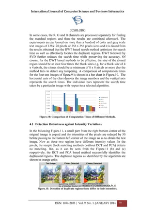
![International Journal of Computer Science and Business Informatics
IJCSBI.ORG
ISSN: 1694-2108 | Vol. 9, No. 1. JANUARY 2014 102
5. CONCLUSION AND FUTURE SCOPE
Cloning or copy-move forgery is one of the widely used image tampering
methods. In this paper we have discussed different methods of cloning
detection those successfully detect duplicated blocks in uncompressed
images. We also have shown how the time complexity of the algorithms can
be improved through DWT, SVD and how the DCT and PCA based
methods can be effetely used to detect duplicated blocks even after
brightness and contrast adjustments performed to the copy-pated regions.
However, these methods fail to detect tampering in JPEG compressed
images and unfortunately nowadays, almost all images are available in
JPEG format. We are trying to extend our work to detect tampering in JPEG
images as well.
REFERENCES
[1] Minati Mishra & MC Adhikary, “Digital Image Tamper Detection Techniques: A
Comprehensive Study”, International Journal of Computer Science and Business
Informatics (ISSN: 1694-2108), Vol. 2, No. 1, Pp. 1-12, JUNE 2013.
[2] The Oxford dictionary online. http://oxforddictionaries.com
[3] Hany Farid, “Image Forgery Detection: A survey”, IEEE signal processing
magazine, March 2009, Pp: 16-25.
[4] Kusam, Pawanesh Abrol and Devanand, “Digital Tampering Detection
Techniques: A Review”, BVICAM‟s International Journal of Information
Technology, Vol.1, No.2,
[5] J. Fridrich, D. Soukal, and J. Lukáš, “Detection of Copy- Move Forgery in Digital
Images”, In Proceedings of the Digital Forensic Research Workshop, Cleveland,
OH, August 2003.
[6] A. C. Popescu and H. Farid, “Exposing digital forgeries by detecting duplicated
image regions”, Technical Report, TR2004-515, Dartmouth College, Computer
Science, 2004.
[7] Farid, H., Lyu, S.: Higher-order wavelet statistics and their application to digital
forensics. In: IEEE Conference on Computer Vision and Pattern Recognition
Workshop (2003).
[8] Amara Graps, “An Introduction to Wavelets”, IEEE Computational Service and
Engineering, 1992, 2(2):50-61
[9] Guohui Li, Qiong WuI, Dan Tu, Shaojie Sun, “A Sorted Neighbourhood Approach
for Detecting Duplicated Regions in Image Forgeries Based on DWT and SVD”,
ICME 2007, 1750-1753.
[10] K. Baker, "Singular Value Decomposition Tutorial", 2005.Available at
http://www.cs.wits.ac.za/~michael/SVDTut.pdf
[11] http://en.wikipedia.org/wiki/Principal_component_analysis
This paper may be cited as:
Mishra, M. and Adhikary, M. C., 2014. Detection of Clones in Digital
Images. International Journal of Computer Science and Business
Informatics, Vol. 9, No. 1, pp. 91-102.](https://image.slidesharecdn.com/vol9no1-january2014-171208072155/85/Vol-9-No-1-January-2014-105-320.jpg)
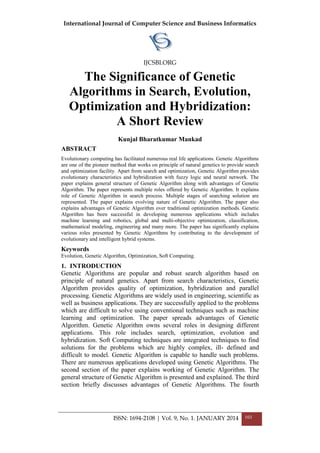
![International Journal of Computer Science and Business Informatics
IJCSBI.ORG
ISSN: 1694-2108 | Vol. 9, No. 1. JANUARY 2014 104
section represents multiple roles associated with Genetic Algorithms. These
roles include search capabilities, evolving capabilities, optimization and
hybridization. The paper explains various roles provided by Genetic
Algorithm. Comparison provided by traditional optimization algorithm and
Genetic Algorithm is presented. The role of Genetic Algorithm is explained
for hybridization with neural network and fuzzy logic. The final section of
the paper justifies significance of multiple roles of Genetic Algorithm by
providing summery of applications developed so far using Genetic
Algorithm.
2. GENETIC ALGORITHM
In recent years, cognitive systems have gained prominence by implementing
evolutionary approach to the computational modeling. The evolutionary
computation is best suited to following types of computational problems
that require following [1]: search through many possibilities to find a
solution, large search space. Parallel approaches are highly suitable for such
problems, an adaptive algorithm.
Genetic Algorithm is an evolutionary-based search or optimization
techniques that performs parallel, stochastic, but direct search method to
evolve the best solution. The area of GA has been traversed by three
prominent researchers namely Fraser in 1962, Bremermann in 1962 and
Holland in 1975 [2,3,4]. Genetic Algorithms are pioneered by John Holland
in 1970’s [5]. Genetic Algorithms are based on principle of natural
evolution which is popularly known as “Darwinian Evolution”.
GA is a population based search algorithm which consists of several
components.
Population of chromosome- Population of chromosome is basically
problem representation using encoding schemes.
Fitness evaluation: A fitness score is allocated to each solution. The
individual with the optimal fitness score is required to be found.
Genetic operations: The entire population evolves towards better
candidate solutions via the selection operations and genetic operators
such as crossover mutation and selection.
Crossover and Mutation: These operators are responsible to generate
new solutions.
Selection: It is responsible to select parent chromosome from available
chromosome. These parent chromosomes will be processed further to
generate new children chromosomes.](https://image.slidesharecdn.com/vol9no1-january2014-171208072155/85/Vol-9-No-1-January-2014-107-320.jpg)
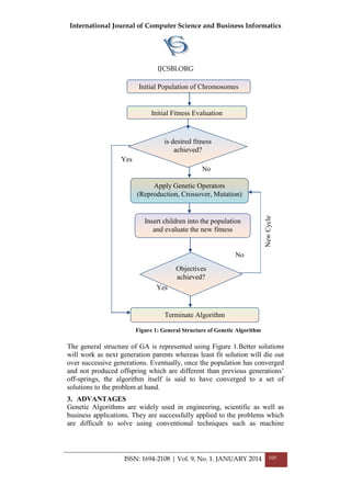
![International Journal of Computer Science and Business Informatics
IJCSBI.ORG
ISSN: 1694-2108 | Vol. 9, No. 1. JANUARY 2014 106
learning and optimization. The major benefit of GA is that it can be used to
find optimized values from large search space as well as makes system able
to learn. It is observed that GA provides following major advantages [6, 7]:
GA can be easily interfaced to obtainable simulations and models;
GA is easy to hybridize and easy to understand;
GA uses little problem specific code;
GA is modular, separate from application;
GA is capable to obtain answers always and gets better with time;
GA is inherently parallel and easily distributed;
GA optimizes with continuous or discrete variables;
GA deals with a large number of variables;
GA provides a list of optimal variables, not just a single solution;
GA encode the variables so that the optimization is done with the
encoded variables; and
GA works with numerically generated data, experimental data, or
analytical functions.
Genetic Algorithms become highly popular in the designing hybrid
intelligent systems and evolutionary systems. In the field of robotics,
Genetic Algorithms have been proven highly successful.
4. MULTIPLE ROLES OF GENETIC ALGORITHM
Compared to traditional search algorithm, Genetic Algorithm plays multiple
roles. These roles include robust search process, evolutionary
characteristics, quality of providing optimization and quality for providing
hybridization with other constituents of soft computing. Due to
aforementioned roles, GA is highly successful in solving real life
applications. The major application areas such as combinatorial search,
intelligent system design, machine learning, and evolutionary robotics have
been gaining proficient results due to capabilities of Genetic Algorithm.
4.1 Role of GA in Search
GA does not require any problem specific knowledge of the search space
because strings are evaluated with fitness quality and hence search is made
possible through the strings which are basically constituents of its structure.
Figure 2 shows process of searching solutions through fitness measures.](https://image.slidesharecdn.com/vol9no1-january2014-171208072155/85/Vol-9-No-1-January-2014-109-320.jpg)
![International Journal of Computer Science and Business Informatics
IJCSBI.ORG
ISSN: 1694-2108 | Vol. 9, No. 1. JANUARY 2014 107
Figure 2: Search Solutions through Fitness Measure
This type of search has capability to move towards multiple directions.
Here, the fitness is measured at one point of time and at the same time
population can be evolved also to next generation. This way parallel
processing is possible. Hence, GA is highly successful in providing
solutions for parallel processing problems.
4.2 Role of GA in Evolving Solutions
The area of evolutionary computation includes the study of the foundations
and the applications of computational techniques based on the principles of
natural evolution. Basically, evolutionary techniques can be considered as
either as search methods, or as optimization techniques [8]. There exist a
number of evolutionary techniques whose main similarity is the use of a
population of random or pseudo-randomly generated solutions to a problem.
A number of operators are applied to the individuals of the current
population to generate the individuals for the next generation population at
each of the iteration. Usually, Genetic Algorithm use an operator called
recombination or crossover to recombine two or more individuals to
produce new individuals. Mutation or modification operators are used to
create a self-adaptation of individuals. In order to select chromosome
(parents) who will generate children chromosomes in next generations,
selection process is designed.
The main categories of selection methods are as follows [9]:
Artificial selection: A selection process is designed such a way that it can
retain or eliminate specific features according to a goal.
Natural selection: According to natural phenomena, the individual who
possesses better existence qualities is able to survive for a longer period of
time. In such cases, better children can be reproduced with genetic material.
A selection process is similar to the Darwinian Theory of biological
evolution. In natural selection process, there is no actor who does the
selection. The selection is purely automatic or spontaneous without any
Solution
S1
• Fitness
Measure
Solution
S2
• Fitness
Measure
Solution
S3
• Fitness
Measure
Solution
S4
• Fitness
Mesure
Solution Sn](https://image.slidesharecdn.com/vol9no1-january2014-171208072155/85/Vol-9-No-1-January-2014-110-320.jpg)
![International Journal of Computer Science and Business Informatics
IJCSBI.ORG
ISSN: 1694-2108 | Vol. 9, No. 1. JANUARY 2014 108
predefined logic. Genetic Algorithm simulates process of natural selection.
Figure 3 represents steps of natural selection process.
Figure 3: Steps of Simulating Natural Selection Process
4.3 Role of GA in Optimization
Optimization is the process of finding decisions that satisfy given
constraints, and meet a specific outcome in terms of its optimal value.
Traditional methods of optimization include both gradient based as well as
direct search techniques. Being one of the prominent representatives of
evolutionary computation, Genetic Algorithm satisfies the requirement
providing optimum solution. The objective of global optimization is to find
the "best possible" solution in nonlinear decision models that frequently
have a number of sub-optimal (local) solutions [10]. In the absence of
global optimization methods, feasible solutions are only the solutions. There
are significant differences observed between GA and most of the traditional
optimization algorithms as summarized by [11,12,13,14]:
Traditional optimization method uses single point approach while GA
uses a population of multiple points at single run;
In traditional optimization, convergence to an optimal solution
depends on the chosen initial solution while in GA, due to randomness
, initial solution is always different;
A classical algorithm is efficient in solving one problem but the same
may not be efficient in solving a different problem while GA is
generic in nature for similar types of objective functions;
GA converts design space into genetic space;
GA works with coding of parameter set rather than actual value of
parameters;
A traditional algorithm may not be efficient to handle problems with
discrete variables or highly non-linear variables with constraints while
GA can be robustly applied to problems with any kinds of objective
functions, such as nonlinear or step functions; because only values of
the objective function for optimization are used to select genes;
Traditional algorithm can stuck at suboptimal solutions while GA can
have less chance to be trapped by local optima due to characteristics of
crossover and mutation operators; and
GA uses stochastic reproduction schemes rather that deterministic
ones.
Representation of
Chromosomes
Data Structure of
Individual
Selection process
of Parent
Chromosome](https://image.slidesharecdn.com/vol9no1-january2014-171208072155/85/Vol-9-No-1-January-2014-111-320.jpg)
![International Journal of Computer Science and Business Informatics
IJCSBI.ORG
ISSN: 1694-2108 | Vol. 9, No. 1. JANUARY 2014 109
The working of Genetic Algorithms for optimum solution is shown in
Figure 4. Due to its random nature, the Genetic Algorithm improves the
chances of finding a global solution [14]. Quite often, several applications
require several contradicting criterions to be satisfied simultaneously. These
problems are known as multi-objective optimization. Often those criterions
are contradicting and cannot have optimum at the same time, thus
improving the value one-criterion means getting worst values for another
[15]. Genetic Algorithms are capable to solve problems of multi-objective
optimization.
4.4 Role of GA in Hybridization
Soft Computing (SC) is not merely a clearly defined field but also a
discipline that deals with hybrid intelligent systems [16]. SC techniques are
integrated techniques to find solutions for the problems which are highly
complex, ill- defined and difficult to model. The family of soft computing is
constructed using four prime techniques: namely Fuzzy Logic (FL),
Evolutionary Computation (EC), Neural Networks (NN) and Probabilistic
Reasoning (PR). Each method is capable of providing distinguished as well
as sharable advantages and obviously carries certain weaknesses also. They
are considered complementary rather than competitive as desirable features
lacking in one approach are present in another. Recent years have
contributed to large number of new hybrid evolutionary systems. There are
several ways to hybridize a conventional evolutionary algorithm for solving
optimization problems. Evolutionary computing is based on Evolutionary
Algorithms (EA). Genetic Algorithms being one of the prominent types of
EA were not specifically designed as machine learning techniques like other
approaches such as neural networks but have been successfully applied to
many search, combinatorial and optimization problems. However, it is well
Figure 4: Working of GA for Optimum Solutions
GA
Model
Experimental Research
& Mathematical
Analysis
Numerical
Modeling
Mathematical
Equation
Solution 1
Solution 2
Solution 3
………
Solution n…
Searching for
optimum
Solutions
Optimum
Solution](https://image.slidesharecdn.com/vol9no1-january2014-171208072155/85/Vol-9-No-1-January-2014-112-320.jpg)
![International Journal of Computer Science and Business Informatics
IJCSBI.ORG
ISSN: 1694-2108 | Vol. 9, No. 1. JANUARY 2014 110
known that a learning task can be modeled as an optimization problem, and
thus can be solved through evolution which is efficiently offered by EA
[17].However, one of the significant limitations of GA; shown in the Table
1 is an inability of storing and handling imprecision. In order to remove
these limitations hybridization of GA with Fuzzy Logic and hybridization of
GA with Neural Network is required respectively.
Table 1: Advantages and Limitations of Constituents of SC
GA-FL Hybridization
In order to have learning and dealing with imprecise knowledge handling,
GA is hybridized with FL. This is popularly known as Genetic-Fuzzy
Hybridization. GA is able to encode and to evolve rule antecedent
aggregation operators, different rule semantics, rule- based aggregation
operators and de-fuzzification methods [18]. Hence, it is considered as
knowledge acquisition scheme. Due to the mentioned qualities optimization
of Fuzzy Rule Based Systems (FRBSs) is made possible. These optimized
Fuzzy Rule Based Systems are capable to design decisions regarding the
characteristics and performance measure [19].
GA-NN Hybridization
GA has been integrated with Neural Network to develop Genetic-Neural
systems. In this type of hybridization, Genetic Algorithms are used to
improve performance of Neural Networks. Several important applications
have been developed using this type of hybrid structures. This type of
hybridization includes following ways of designing Genetic-Neural systems
[20]:
GA based tuning of connecting weights, bias values and other
parameters.
GA based tuning of neural network topologies.
GA based preprocessing of data and interpretation of the output of NN.
Constituents
of SC
Advantages Limitations
GA Natural evolution and
optimization
Inability of storing and
handling imprecision
FL Approximate reasoning,
imprecision
Inability of learning
NN Learning and implicit
knowledge
representation
Inability for optimization
PR Uncertainty Inability of learning](https://image.slidesharecdn.com/vol9no1-january2014-171208072155/85/Vol-9-No-1-January-2014-113-320.jpg)
![International Journal of Computer Science and Business Informatics
IJCSBI.ORG
ISSN: 1694-2108 | Vol. 9, No. 1. JANUARY 2014 111
GA-PR Hybridization
The aim of a probabilistic logic (also probability logic and probabilistic
reasoning) is to combine the capacity of probability theory to handle
uncertainty with the capacity of deductive logic to exploit structure.
Integration of Genetic Algorithm with Probabilistic Reasoning (PR) has not
been widely popular so far. Bayesian Network is the most popular approach
of PR. In order to find optimal structure of Bayesian network for a given
database of training cases, GA is utilized. Bayesian optimization algorithms
are designed with help of GA-PR hybridization [18].
5. LITERATURE REVIEW OF APPLICATIONS USING GA
As a result of extensive literature survey; it has been observed that GA has
been successfully applied to real life application areas
[14,18,21,22,23,24,25,26,27,28, 29,30,31,32,33,34,35]. The summarized
information of major applications developed using implementation of
Genetic-Algorithm is represented in Table 2.
Table 2: Summarizing Major Applications of Genetic Algorithm
Application
Domain
Example of Applications
Global
Optimization
Travelling Salesperson Problems consists of
following:
Ex. routing of school buses, airlines, trucks, postal
carriers
Prediction Weather Forecasting, Financial Forecasting,
Marketing & Sales
Scheduling
Problems
Effective Distribution of Resources, Examples:
Timetabling problems, railway scheduling problems
Job shop Scheduling problems
Machine Learning Classification problems
Automated knowledge acquisition problems
Example based learning algorithms
Learning Robot Behavior
Multi-Objective
Optimization
Decision making problems in transportation
planning and management
Engineering
Problems
Designing intrusion detection in network, mobile
telecommunication networks, etc.
Applications in Mechanics, hydrodynamics,
aeronautics, etc.
Dynamic Data
Analysis
Continuous Analysis of event such as change in
stock prices, fashion industry, and any other real](https://image.slidesharecdn.com/vol9no1-january2014-171208072155/85/Vol-9-No-1-January-2014-114-320.jpg)
![International Journal of Computer Science and Business Informatics
IJCSBI.ORG
ISSN: 1694-2108 | Vol. 9, No. 1. JANUARY 2014 112
application
Classification Text Mining, information retrieval, Rule
Discovery
Computer Games Real time computer games
Automation In Object Oriented Software Engineering, unit test
cases are generated automatically
Computer automated design
Mathematical
Modeling
Graph coloring problems, artificial vision system
Hybrid Systems Evolutionary–fuzzy system for robotics, decision
making, medical diagnostic system
Neural-Genetic-Fuzzy Modeling for control
system
Media
Segmentation
Applications of media segmentation includes
image, video, and music segmentation
Some of the major applications from Table 2 are explained as under:
GAs has been successful in achieving solutions for the variety of
scheduling problems which need to deal with effective distribution of
resources. During the scheduling process many constraints have to be
considered [22]. Genetic Algorithm has been also used to solve the train
timetabling problem. The railway scheduling problem considered in this
work implies the optimization of trains on a railway line that is occupied
(or not) by other trains with fixed timetables. The timetable for the new
trains is obtained with a Genetic Algorithm (GA) that includes a guided
process to build the initial population [23].
In the engineering of mobile telecommunication networks, two major
problems can occur in the design of the network and the frequency
assignment. The design of telecommunication network is of the type of
multi-objective constrained combinatorial optimization problem. In
order to achieve this type of optimization, GA is proposed to increase
the speed of the search process; the GA is implemented parallel on a
network of workstations [28].
Genetic Algorithms are designed to play real-time computer strategy
games. Unknown and non-linear search space can be explored using GA
and spatial decision making strategies and population have been
implemented within the individuals of a Genetic Algorithm [31].
Genetic Algorithm has been proven highly successful in large number of
application areas. In order to make GA more effective and efficient, robust
fitness function and effective crossover operator should be designed. GA
has been providing significant advantages searching, optimization and](https://image.slidesharecdn.com/vol9no1-january2014-171208072155/85/Vol-9-No-1-January-2014-115-320.jpg)
![International Journal of Computer Science and Business Informatics
IJCSBI.ORG
ISSN: 1694-2108 | Vol. 9, No. 1. JANUARY 2014 113
evolution. The most promising research area is Genetic Algorithm based
hybrid systems. Hybridization of genetic algorithms have contributed a lot
in designing intelligent systems, robotics, evolutionary systems, machine
learning systems, etc. The solutions provided by Genetic Algorithms are
very rapid, reliable and precise.
6. CONCLUSION
The paper explains Genetic Algorithm and its working characteristics.
Various advantages of Genetic Algorithm are presented. Genetic
Algorithms possesses several important features such as evolution, search,
optimization and hybridization. The paper explains multiple roles of
Genetic Algorithms. One of the major beneficial characteristics of Genetic
Algorithm is to implement efficient search process compared to traditional
search algorithms. Genetic Algorithms are capable to simulate process of
natural evolution. The various steps of natural evolution are presented in
this paper. Genetic Algorithm plays extremely important role in providing
global optimization. The paper explains how Genetic Algorithm is utilized
for achieving optimized outcome compared to traditional optimization
methods. This paper presents advantages and limitations of major
constituents of soft computing family i.e. Genetic Algorithm, fuzzy logic,
neural network and probabilistic reasoning. Being one of the important
constituents of Soft Computing, Genetic Algorithm is greatly advantages in
designing hybrid intelligent systems. The hybrid systems have strength of
each of the technique used in designing the systems. The paper highlights
importance of Genetic-Fuzzy System, Genetic-Neural system, Genetic-
Bayesian system. The literature survey of the applications developed so far
using implementation of Genetic Algorithm includes significant real world
applications. Thus, the paper justifies significance of varied roles of Genetic
Algorithm by providing summery of applications developed so far using
Genetic Algorithm. It also outlines future trends and research direction of
Genetic Algorithms.
REFERENCES
[1] Leung, J. et al. (2011). Genetic Algorithms and Evolution Strategies [Online].
Available:http://pages.cpsc.ucalgary.ca/~jacob/Courses/Winter2000/CPSC533/Slides/0
4.3.1-ES-GA.ppt [Accessed: June 2013].
[2] Fraser, A.S., Simulation of genetic systems, J. Theoretical Biology, vol. 2, no.3, pp.
329- 346, May 1962.
[3] Bremermann, H. J., Optimization through evolution and recombination, in Self –
organizing Syst., M.C. Yovits, et al., Eds. Washington D.C.: Spartan Books, 1962, pp.
93-106.
[4] Holland, J. H., Adaptation in natural and artificial systems. Ann arbor: The University
of Michigan Press, 1975.
[5] Holland, J. H., Hierarchical descriptions of universal spaces and adaptive systems, in
Essays on cellular automata, A.W. Bruks , Ed. Urbana: Univ. Illinois Press,1970, pp.
320-353.](https://image.slidesharecdn.com/vol9no1-january2014-171208072155/85/Vol-9-No-1-January-2014-116-320.jpg)
![International Journal of Computer Science and Business Informatics
IJCSBI.ORG
ISSN: 1694-2108 | Vol. 9, No. 1. JANUARY 2014 114
[6] Williams, W., Meta-heuristic Algorithms: Genetic Algorithm: A Tutorial
[Online].Available: https://www.cs.drexel.edu/~spiros/teaching/SE320/slides/ga.pdf
[Accessed: May 2013].
[7] Haput, R. and Haput, L., Practical Genetic Algorithms, 2nd
Edition,A JOHN WILEY &
SONS, 2004.
[8] Reyes, C. and Sipper, M., Evolutionary computation in medicine: an overview,
Artificial Intelligence in Medicine, vol. 19, pp.1-23, 2000.
[9] Mankad, K. B. and Sajja, P. S. (July 2012). Measuring human intelligence by applying
soft computing techniques: A genetic fuzzy approach , in Diagnostic Test
Approaches to Machine Learning and Commonsense Reasoning Systems, X.A.
Naidenova and D. Ignatov, Eds. Hershey, PA: IGI Global, pp.128-153 [Online].
Available: http://www.irma-international.org/viewtitle/69407/ [Accessed July 2013].
[10]Bajpai, P. and Kumar, M., Genetic Algorithm – an Approach to Solve Global
Optimization Problems, Indian J. Computer Sci. and Eng., vol. 1, no. 3, pp. 199-206,
Oct.-Nov. 2010.
[11]Karry, F. O. and Silva, C. D. Soft computing and intelligent system design: Theory,
tools and applications, 1st ed., New York, NY: Pearson, 2004, pp. 44, 64, 368,374-
375,379,382,390.
[12]Padhy, N. P., Artificial Intelligence and Intelligent System. New Delhi, India: Oxford
University Press, 2005, pp. 23,279,330-333,363,463,483-499.
[13]Rajsekaran, S. and Pai, V., Neural Networks, Fuzzy Logic, and Genetic Algorithms
Synthesis and Applications. New Delhi: PHI, 2003, pp.11, 228,249.
[14]Deb, K. Revolutionary Optimization by Evolutionary Principles, [online]Available:
http://www.iitk.ac.in/directions/directsept04/deb~new.pdf
[15]Andrey, P. ,Genetic Algorithm for Optimization, User Manual, Hamburg, 2005.
[16]Akerakar, R. and Sajja, P.S. Knowledge-Based Systems. Sudbury, MA: Jones and
Bartlett, 2010, pp. 67,129,152,218,239,243.
[17]Herrera, F. (2009). Lecture Notes for Data Mining and Soft Computing- Session 6,
Genetic-Fuzzy Systems- I. Dept. Computer Science and A.I., University of Granada,
Spain [Online].
Available:http://www.isa.cie.uva.es/estudios/doctorado/documentacion2009/DM-SC-
06-I-Genetic-Fuzzy-Systems.pdf [Accessed: Jan 2014].
[18]Cor'don, O. et al., Genetic Fuzzy Systems Evolutionary tuning and learning of fuzzy
knowledgebases. Singapore: World Scientific, 2001,pp. 1, 2,40,79-80,87,89,130, 132-
136,142-144,375-380,414-416.
[19]Puig, A.O. et al., Evolving Fuzzy Rules with UCS: Preliminary Results, in Learning
Classifier Systems, J. Bacardit et.al., Eds.vol. 4998, Berlin, Heidelberg: Springer-
Verlag, 2008, pp. 57-76.
[20]Pratihar, D. K. Soft Computing. New Delhi: Narosa, 2008.
[21]Valenzuela, C. L. Evolutionary Divide and Conquer: a novel genetic approach to the
TSP, Ph.D. dissertation, Dept. Comput., Univ. London, London, England,1995.
[22]Sigl, B. et al., Solving Timetable Scheduling Problem by Using Genetic Algorithms, in
Proc. 25th Int. Conf. IT Interfaces, June 2003, pp. 519 – 524.
[23]Tormos, P. et al., A Genetic Algorithm for Railway Scheduling Problems, in
Metaheuristics for Scheduling in Industrial and Manufacturing Applications, F. Xhafa
and A.Abraham, Eds. vol.128, Berlin, Heidelberg: Springer, 2008, pp. 255–276.
[24]Fidelis, M. V. et al., Discovering comprehensible classification rules with a Genetic
Algorithm, in Proc. 2000 Congr. Evol. Comput., vol. 1, R. Dienstbier, Ed. July 2000,
pp. 805-810.
[25]Ribeiro, A. et al., Automatic Rules Generation by GA for Eggshell Defect
Classification, presented at Proc. European Congr. Comput. Methods in Appl. Sci. and
Eng., Barcelona , Spain, 2000.](https://image.slidesharecdn.com/vol9no1-january2014-171208072155/85/Vol-9-No-1-January-2014-117-320.jpg)
![International Journal of Computer Science and Business Informatics
IJCSBI.ORG
ISSN: 1694-2108 | Vol. 9, No. 1. JANUARY 2014 115
[26]Srinivas, N. and Deb, K., Multi-objective Optimization Using Non-dominated Sorting
in Genetic Algorithms, Evol .Compu., vol.2, no.3, pp. 221-248,1994.
[27]William, H. K. and Yin, Y., Genetic Algorithm-Based Approach for Transportation
Optimization Problems, in The Practical Handbook of Genetic Algorithms, 2nd Ed., L.
Chambers, Eds. MA: Hall& Chapman/CRC Press, 2000, pp. 236-244.
[28]Meunier, H. et al., A multi-objective Genetic Algorithm for radio network
optimization, in Proc. 2000 Cong. Evol. Compu., vol.1, La Jolla, CA, July 2000, pp.
317- 324.
[29]Li, W. Using Genetic Algorithm for Network Intrusion Detection, in Proc.US. Dept.
Energy Cyber Security Group 2004 Training Conf., Kansas City, Kansas,2004, pp. 24-
27.
[30]Quintana, D. et al., Evolutionary Rule-Based System for IPO Under-pricing Prediction,
in Proc. Genetic and Evo. Comput. Conf., Washington , DC, June 2005, pp. 983-989.
[31]Miles, C. and Louis, S.J., Towards the Co-Evolution of Influence Map Tree Based
Strategy Game Players, in IEEE Symp. Comput. Intell. and Games, May 2006, pp. 75–
82.
[32]Gupta, N. K. and Rohil, M. Using Genetic Algorithm for Unit Testing of object
oriented software, in Proc. First Int. Conf .Emerging Trends in Eng. and Techno., July
2008, pp. 308-313.
[33]Eiben, A. E. and Hauw, J. K., Graph Coloring with Apadtive Genetic Algorithm , J.
Heuristics, vol. 4, no. 1, pp. 25-46, Jun. 1998.
[34]Rafael, B., Affenzeller , M., Wagner, S., Application of an Island Model Genetic
Algorithm for a Multi-track Music Segmentation Problem, in P. Machado, Eds.
Evolutionary and Biologically Inspired Music, Sound, Art and Design,pp.13-24,
Springer Berlin Heidelberg, April 3-5, 2013.
[35]Spanos, A. C.,et.al., A new hybrid parallel genetic algorithm for the job-shop
scheduling problem, International Transactions in Operational Research, Oct 2013,
DOI: 10.1111/itor.12056.
This paper may be cited as:
Mankad, K. B., 2014. The Significance of Genetic Algorithms in Search,
Evolution, Optimization and Hybridization: A Short Review. International
Journal of Computer Science and Business Informatics, Vol. 9, No. 1, pp.
103-115.](https://image.slidesharecdn.com/vol9no1-january2014-171208072155/85/Vol-9-No-1-January-2014-118-320.jpg)