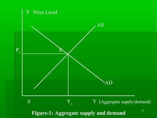
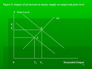
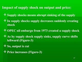
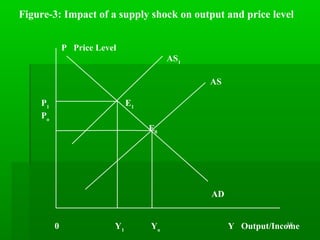
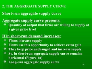
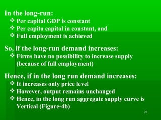
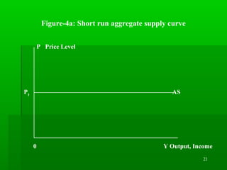
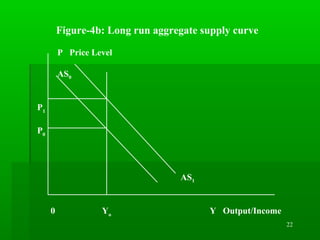
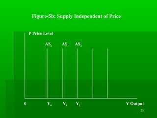
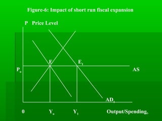
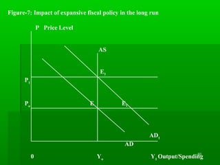
1
AGGREGATE SUPPLY AND AGGREGATE DEMAND
MD Siyam Hossain
Bangladesh Institute of Business & Technology
Narayangonj,Dhaka
Dhaka,Bangladesh
www.facebook.com/mdsiyamhossain
2
1. AGGREGATE SUPPLY AND DEMAND MODEL
 Aggregate Supply-Demand Schedule
Aggregate supply-demand curves are tool for studying:
 Fluctuations in output
 Price level and
 Inflation rate
Aggregate supply-demand curves helps to understand:
 Why the economy deviates from growth path over
time
 Aggregate supply-demand curves helps to investigate
the impact of policies on:
 Employment
 Output, and
 Inflation
3
Aggregate Supply Schedule
Aggregate supply curve (AS) represent:
 Quantity of output firms willing to supply for a given
price levels
 Aggregate Supply curve is upward sloping
Aggregate Supply Says:
 At higher price firms are willing to supply more
output and
 At lower price firms supply les output (Figure-1)
4
Aggregate Demand Schedule
Aggregate demand (AD) Schedule shows that goods and
money markets are in equilibrium at certain (Figure-1):
Price level and
Level of output
Aggregate demand (AD) Schedule is downward sloping
Aggregate demand (AD) Schedule shows that higher
prices:
 Reduce the value of the money and
 Demand for output sinks
 Intersection of the AD and AS Schedule
5
Intersection of the AD and AS determines:
Equilibrium level of output and
Equilibrium level of output price
Intersection of AD and AS at E determines the
equilibrium level of output Yo
, and the equilibrium price
level, Po
(Figure-1)
Shift either of demand and supply schedule
causes:
Change in price level and
Change in output level (Figure-1)
6
P Price Level
AS
Po
E
AD
0 Yo
Y (Aggregate supply/demand)
Figure-1: Aggregate supply and demand
7
Causes for Shifting of Aggregate Demand Schedule
On following grounds the aggregate demand curve shifts:
 Increases in government spending,
 Cuts in taxes
 Increases in the money supply and
 Consumer and investor confidence also
 (i) Increases in government spending
Increase in government spending increases:
 Could increase money supply
As a result:
 Demand of output increases
 And price increases and AD curve moves to the right
8
(i) Cuts in taxes
Tax Cuts:
 Increases ultimate income and demand
 This shifts the demand schedule rightward
As a result:
 Demand of output increases
 Output increases
 And price increases
9
(ii) Increase in confidence of the consumer and investor
Increase in the confidence of the consumer:
 Increase in the confidence of the consumer increases
demand
 The AD curve moves to the right
As a result:
 Demand of output increases
 Output increases
 And price increases
 Increase in the confidence of the investor increases:
 Increase in the confidence of the investor increases
investment
10
As a result:
 Output increases,
 Demand increases
 And price increases
 The AD curve moves to the right
 When confidence of consumer and investor drops
demand
 Demand decreases
 Output decreases
 Price decreases
 The AD curve moves to the left
11
(iii) Increases in the money supply
Increase in money supply is only then real money supply,
when:
 Money supply increases the value of the money
 That is, when money supply increases real income
 When money supply increases income then it is
called real money supply
Increases in the real money supply:
 Increases income
 Increases demand
 Increases output
 Increases price
12
Condition of real money supply
 Real money supply depends on the value of M/P
 Where M is money supply and P is price level
 So, when M/P increases, real money supply increases
 That is, when increase in money supply (M) more
than price (P) increases
 When M/P decreases, real money supply decreases
 That is, when price (P) increase is more than money
supply (M)
13
When money supply causes real money supply, then:
 Interest rate falls
 Investment rises
 Output also increases
 Real income increases
 Aggregate demand increase
On the contrary, when money supply decreases value of
money:
 Interest rate increases
 Investment decreases
 Output also decreases
 Real income decreases
 Aggregate demand decreases
14
ANALYSING BEHAVIOUR OF THE SUPPLY AND DEMAND
CURVE
Let us suppose that the government increases the
money supply
What impact will have this on the price level?
Will have the increase in the money supply cause
inflation?
Will the output increase?
Or do both output and the price level rise?
15
An increase in the money supply:
 Shifts the aggregate demand curve AD to the right to
AD1
(Figure-2)
 Shifting of aggregate demand curve moves
equilibrium of economy from E to E1
 The price level rises from Po
to P1
 This shifting moves also the level of output from Yo
to Y1
 Increase in money supply increases level of output
and price (Figure-2)
16
Figure-2: Impact of an increase in money supply on output and price level
P Price Level
AS
P1
Po
E1
E
0 Yo
Y1
Demanded Output
17
Impact of supply shock on output and price:
 Supply shocks means abrupt sinking of the supply
 In supply shocks supply decreases suddenly creating
shock
 OPEC oil embargo from 1973 created a supply shock
 As by supply shock supply sinks, supply curve shifts
leftward (Figure-3)
 So, output is cut
 Price increases (Figure-3)
18
Figure-3: Impact of a supply shock on output and price level
P Price Level
AS1
AS
P1
E1
Po
E0
AD
0 Y1
Yo
Y Output/Income
19
2. THE AGGREGATE SUPPLY CURVE
Short-run aggregate supply curve
Aggregate supply curve presents:
 Quantity of output that firms are willing to supply at
a given price level
If in short-run demand increases:
 Firms increase supply
 Firms use this opportunity to achieve extra gain
 They keep price unchanged and increase supply
 So, in short-run aggregate supply curve remains
horizontal (Figure-4a)
 Long-run aggregate supply curve
20
In the long-run:
 Per capital GDP is constant
 Per capita capital in constant, and
 Full employment is achieved
So, if the long-run demand increases:
 Firms have no possibility to increase supply
(because of full employment)
Hence, if in the long run demand increases:
 It increases only price level
 However, output remains unchanged
 Hence, in the long run aggregate supply curve is
Vertical (Figure-4b)
21
Figure-4a: Short run aggregate supply curve
P Price Level
P1
AS
0 Y Output, Income
22
Figure-4b: Long run aggregate supply curve
P Price Level
AS0
P1
P0
AS1
0 Yo
Y Output/Income
23
2.1 CHANG OF AGGREGATE SUPPLY CURVE OVER TIME
 Over time the economy accumulates resources, technology
improves and GDP grows
 So, over time aggregate supply curve moves to the right
(Figure-5a Figure-5b)
 The Changes of GDP over a short period is usually small
(Bangladesh 5%)
 So, a single vertical line can be drawn to represent short-run
supply of GDP
 Annual changes of GDP do not depend on the price level
 Annual supply of GDP is ‘exogenous to the price level’
(Figure-5b)
24
Figure-5a: Output Change Over Time
Y Output
Y2
Y1
Y0
0 to
t1
t2
Time
25
Figure-5b: Supply Independent of Price
P Price Level
ASo
AS1
AS2
0 Y0
Y1
Y2
Y Output
26
2.2 SHORT RUN (KEYNESIAN) AGGREGATE
SUPPLY CURVE
 The idea of short run supply curve implies that
there is unemployment
 The firms can obtain as much labour as they want
at present wage
 So, the costs of production do not to change as
output levels change
 Firms are willing to supply as much as demanded
at existing price
 So, short run (Keynesian) aggregate supply is
horizontal
 This indicates that firms supply whatever
demanded at the existing price
27
2.3 FRIC11ONAL OR NATURAL UNEMPLOYMENT
 Classical model implies that there is no
unemployment
 Everyone who wants to work get work
 But practically there is always some
unemployment
 This unemployment is associated with
market friction
 Labour market is in continuous change
 Some people are moving and changing jobs
 Other looking for jobs
28
 Some firms are expanding and hiring new workers
 Others firms reduce employment by firing workers
 Under such condition to find the right job toilsome
 So, there is always some frictional unemployment
 Frictional unemployment exists because of shifting
one job and for new
 Such unemployment is also called the natural
unemployment
 It exists when the labour market is in equilibrium
 Currently natural rate in United States is about
5.5%
In spite of some frictional unemployment, we can say
there is full employment:
 If those who wish to work are able to get work
29
2.4 STRUCTURAL UNEMPLOYMENT
 In modem economy, man by himself hardly produces
anything
 Even primitive man needed some tools like bow and
arrow for his livelihood
 With growth of technology, much more capital
needed for productive activity
 All instruments of production constitute stock of
capital
 Now, if working force grows faster than capital stock
of a country, entire labour force cannot be absorbed
in productive employment
 So, some will remain unemployed
 Such unemployment is known as structural
(Marxian) unemployment
30
2.5 SEASONAL UNEMPLOYMENT
 Some productive activity has seasonal character
 In these sectors (activities), during the slack season
people become unemployed
 Such unemployment is known as seasonal
unemployment
 Agriculture work is normally a seasonal occupation
 So, farmers have not sufficient work to do during
the slack season
 Other examples of seasonal industry are:
 Ice factories
 Rice mills
 Sugar factories, etc
31
2.6. KEYNESIAN UNEMPLOYMENT OR CYCLICAL
UNEMPLOY-MENT
 Equilibrium level of income and employment may be
established at less than full employment level
 That means, there is some unemployment
 It is known as Keynesian unemployment
 It is due to deficiency of aggregate effective demand
 It is also called cyclical unemployment
 It is called cyclical, because business depression
occurs at cyclical intervals
 During depression, business activity is at low ebb and
unemployment increases
 Some people are thrown out of employment
altogether
 Some are partially employed
32
 This type of unemployment arises not because of too
little capital as for structural unemployment
 It occurs because of too much capital
 This type of unemployment occurs because total
effective demand is not sufficient to absorb the entire
production of goods that can be produced with the
available stock of capital
 Business cannot sell their entire output
 So, output is reduced that occurs creates
unemployment
33
Measures Removing Cyclical or Keynesian Unemployment
 This unemployment is due to the deficiency of effective
demand
 It could be removed by boosting effective demand
 Boosting effective demand following should be done:
 Government boost consumption by reducing tax rates
on incomes and consumption
 Government subsidies private consumption
 Government increases its own consumption
34
4. FISCAL AND MONETARY POLICY UNDER
ALTERNATIVE SUPPLY ASSUMPTIONS
4.1 SHORT RUN (KEYNESIAN) FISCAL POLICY
Fiscal policy includes govt income (tax) and
expenditure policy
The fiscal policy could be expansionary or contractive
Expansionary fiscal policy includes tax cut and
expansion of the market
Contractive fiscal policy includes increasing tax and
cutting market
Let the market is equilibrium in at point E (Figure-6)
At point E the aggregate demand and supply
schedules intersect
Let us now consider a short run change
35
 Let us consider a fiscal expansion
 Let government expands spending (or cut tax)
 Demand increases and shifts rightward from AD to
AD1
(Figure-6)
 As it is a short run change, supply schedule is a
horizontal line AS passing through E
 The Supply schedule intersects the new demand
schedule at equilibrium point E1
 Output increases, but no prices increase (Figure-6)
 Impact of higher government spending (or tax cut) is:
 Increase in output (Y1)
 No prices increase (P0)
 Generate employment
36
Figure-6: Impact of short run fiscal expansion
P Price Level
E E1
Po
AS
AD1
0 Yo
Y1
Output/Spending
37
4.2 IMPACT OF LONG RUN FISCAL POLICY
 Let us analyse the impact of fiscal policy in the long
run
 Fiscal policy includes govt income (tax) and
expenditure policy
 Fiscal policy could be expansionary or contractive
 Expansionary fiscal policy means tax cut and
expansion of the market
 Contractive fiscal policy means increasing tax and
cutting market
 Let us consider that government follows an
expansionary fiscal policy
 Let government expands spending
38
 In long run the aggregate supply curve is vertical
 Supply cannot be increased because there is full-
employment
 Level of output (Y*) remains constant (Figure-7)
 Impact of Expansionary fiscal policy in the long run
is:
 No increase in output
 Per capital GDP remains constant
 Price increase
 Let us consider that government follows an
expansionary fiscal policy
It cuts tax, so:
 Demand increases and demand schedule shifts
rightward from AD to AD1
39
 If there is unemployment economy move to E1
in short
run
 Supply increase by unchanged price P0
to E1
 Firms cannot obtain labour to produce more output
New demand schedule intersects the vertical aggregate
supply schedule at point E2
 This is new equilibrium and at point E2
there is full
employment
 Supply of output cannot be increased to meet
increased demand
 Firms charge higher prices for their output and price
increases
 Impact of tax cut in the long run is:
No increase in output
Price increase
40
Figure-7: Impact of expansive fiscal policy in the long run
P Price Level
AS
E1
P1
Po
E E1
AD1
AD
0 Yo
Y1
Output/Spending
41
The process of price increase:
 Let before the tax cut the real money stock was M/P
 M was money supple, P was the price level and there
was equilibrium
 Let because of tax cut money supply increases to M1
 Demand increases
 Output can’t be increased
 So, price level increases
Price level increases to P1
so that:
 M/P = M1
/P1
 There is new equilibrium at higher price (P1)
 That means, same output is supplied at higher price
42
4.2.1 Crowding Out
 Let there was equilibrium between government and
private sector spending
 Let now government spends more
 (Govt either increases tax or borrows from bank)
 So, private sector spends less
 (Because the total income is constant)
 Spending of private sector falls by amount that
government spends more
 This is known as crowding out
 Crowding out occurs when increase in government
spending lessens private sector spending
 There is full or partial crowding out
43
5. ONGOING MONEY GROWTH AND INFLATION
IN LONG RUN
 In long run money supply leads to increase price
level
 If money supply grows 10% a year
 Demand schedule would move up 10% annually
 Point of equilibrium of demand and supply would
move up 10%
 It means, in the long run prices would rise 10%
annually
 So we see ongoing money growth leads to inflation
 In the long run fiscal policy cannot affect output
 So, neutrality of money has strong policy
implications
44
 If money were neutral, inflation could be reduced
 For this, growing of the money stock would have to be
stopped
 In practice, it is difficult to reduce inflation without
recession
 Lower growth rate of money leads to demand sinks
 Consequently, output sinks and unemployment
increases
 So, money is not neutral
 Changes in quantity of money have real effects
 Monetary policy affects the level of output
45
6. SUPPLY-SIDE ECONOMICS
Some economists favour policies:
 Those shift supply curve right ward
 And increases GDP
Arguments are:
 Increased supply creates job
 And increases per capita income
46
So, following policies suggested for increasing supply:
 Removing unnecessary regulation of the economy
 Cutting tax rates
 Encouraging technological progress
 Some economists refer ‘supply-side economics’ as
‘voodoo (curse) economics’
Let us analyse what happens if tax rates are cut
 Tax cut has effects both on aggregate supply and
aggregate demand
 Aggregate demand increases
 (Demand schedule shifts right from AD to
AD1
/Figure-7)
47
 This shift is relatively large
 Aggregate supply also increases
 (Supply curve shifts to the right from AS to
AS1
/Figure -7)
 Lower tax rates increase the incentive to work
 The effect of such an incentive is quite small
 So, rightward shift of GDP is small
 So, in short run GDP is higher but very small amount
 However, total tax collections fall and the deficit rises
 In addition, prices are permanently higher
48
Supply Side Economics: Experiences in the USA
Tax was cut in USA in 1981-1983
 Output increased very small
 Price increased
 Budget deficit increased
 Many economists don't believe in magic of tax cut
 Conservative economists argue that tax cut has a
small but real effective incentive
 They suggest that cutting of tax & govt spending
should fall at same time:
 Tax collections fall, so fall also government
spending
 So, effect on budget is nearly neutralised

Aggregate supply and aggregate demand

  • 1.
    1 AGGREGATE SUPPLY ANDAGGREGATE DEMAND MD Siyam Hossain Bangladesh Institute of Business & Technology Narayangonj,Dhaka Dhaka,Bangladesh www.facebook.com/mdsiyamhossain
  • 2.
    2 1. AGGREGATE SUPPLYAND DEMAND MODEL  Aggregate Supply-Demand Schedule Aggregate supply-demand curves are tool for studying:  Fluctuations in output  Price level and  Inflation rate Aggregate supply-demand curves helps to understand:  Why the economy deviates from growth path over time  Aggregate supply-demand curves helps to investigate the impact of policies on:  Employment  Output, and  Inflation
  • 3.
    3 Aggregate Supply Schedule Aggregatesupply curve (AS) represent:  Quantity of output firms willing to supply for a given price levels  Aggregate Supply curve is upward sloping Aggregate Supply Says:  At higher price firms are willing to supply more output and  At lower price firms supply les output (Figure-1)
  • 4.
    4 Aggregate Demand Schedule Aggregatedemand (AD) Schedule shows that goods and money markets are in equilibrium at certain (Figure-1): Price level and Level of output Aggregate demand (AD) Schedule is downward sloping Aggregate demand (AD) Schedule shows that higher prices:  Reduce the value of the money and  Demand for output sinks  Intersection of the AD and AS Schedule
  • 5.
    5 Intersection of theAD and AS determines: Equilibrium level of output and Equilibrium level of output price Intersection of AD and AS at E determines the equilibrium level of output Yo , and the equilibrium price level, Po (Figure-1) Shift either of demand and supply schedule causes: Change in price level and Change in output level (Figure-1)
  • 6.
    6 P Price Level AS Po E AD 0Yo Y (Aggregate supply/demand) Figure-1: Aggregate supply and demand
  • 7.
    7 Causes for Shiftingof Aggregate Demand Schedule On following grounds the aggregate demand curve shifts:  Increases in government spending,  Cuts in taxes  Increases in the money supply and  Consumer and investor confidence also  (i) Increases in government spending Increase in government spending increases:  Could increase money supply As a result:  Demand of output increases  And price increases and AD curve moves to the right
  • 8.
    8 (i) Cuts intaxes Tax Cuts:  Increases ultimate income and demand  This shifts the demand schedule rightward As a result:  Demand of output increases  Output increases  And price increases
  • 9.
    9 (ii) Increase inconfidence of the consumer and investor Increase in the confidence of the consumer:  Increase in the confidence of the consumer increases demand  The AD curve moves to the right As a result:  Demand of output increases  Output increases  And price increases  Increase in the confidence of the investor increases:  Increase in the confidence of the investor increases investment
  • 10.
    10 As a result: Output increases,  Demand increases  And price increases  The AD curve moves to the right  When confidence of consumer and investor drops demand  Demand decreases  Output decreases  Price decreases  The AD curve moves to the left
  • 11.
    11 (iii) Increases inthe money supply Increase in money supply is only then real money supply, when:  Money supply increases the value of the money  That is, when money supply increases real income  When money supply increases income then it is called real money supply Increases in the real money supply:  Increases income  Increases demand  Increases output  Increases price
  • 12.
    12 Condition of realmoney supply  Real money supply depends on the value of M/P  Where M is money supply and P is price level  So, when M/P increases, real money supply increases  That is, when increase in money supply (M) more than price (P) increases  When M/P decreases, real money supply decreases  That is, when price (P) increase is more than money supply (M)
  • 13.
    13 When money supplycauses real money supply, then:  Interest rate falls  Investment rises  Output also increases  Real income increases  Aggregate demand increase On the contrary, when money supply decreases value of money:  Interest rate increases  Investment decreases  Output also decreases  Real income decreases  Aggregate demand decreases
  • 14.
    14 ANALYSING BEHAVIOUR OFTHE SUPPLY AND DEMAND CURVE Let us suppose that the government increases the money supply What impact will have this on the price level? Will have the increase in the money supply cause inflation? Will the output increase? Or do both output and the price level rise?
  • 15.
    15 An increase inthe money supply:  Shifts the aggregate demand curve AD to the right to AD1 (Figure-2)  Shifting of aggregate demand curve moves equilibrium of economy from E to E1  The price level rises from Po to P1  This shifting moves also the level of output from Yo to Y1  Increase in money supply increases level of output and price (Figure-2)
  • 16.
    16 Figure-2: Impact ofan increase in money supply on output and price level P Price Level AS P1 Po E1 E 0 Yo Y1 Demanded Output
  • 17.
    17 Impact of supplyshock on output and price:  Supply shocks means abrupt sinking of the supply  In supply shocks supply decreases suddenly creating shock  OPEC oil embargo from 1973 created a supply shock  As by supply shock supply sinks, supply curve shifts leftward (Figure-3)  So, output is cut  Price increases (Figure-3)
  • 18.
    18 Figure-3: Impact ofa supply shock on output and price level P Price Level AS1 AS P1 E1 Po E0 AD 0 Y1 Yo Y Output/Income
  • 19.
    19 2. THE AGGREGATESUPPLY CURVE Short-run aggregate supply curve Aggregate supply curve presents:  Quantity of output that firms are willing to supply at a given price level If in short-run demand increases:  Firms increase supply  Firms use this opportunity to achieve extra gain  They keep price unchanged and increase supply  So, in short-run aggregate supply curve remains horizontal (Figure-4a)  Long-run aggregate supply curve
  • 20.
    20 In the long-run: Per capital GDP is constant  Per capita capital in constant, and  Full employment is achieved So, if the long-run demand increases:  Firms have no possibility to increase supply (because of full employment) Hence, if in the long run demand increases:  It increases only price level  However, output remains unchanged  Hence, in the long run aggregate supply curve is Vertical (Figure-4b)
  • 21.
    21 Figure-4a: Short runaggregate supply curve P Price Level P1 AS 0 Y Output, Income
  • 22.
    22 Figure-4b: Long runaggregate supply curve P Price Level AS0 P1 P0 AS1 0 Yo Y Output/Income
  • 23.
    23 2.1 CHANG OFAGGREGATE SUPPLY CURVE OVER TIME  Over time the economy accumulates resources, technology improves and GDP grows  So, over time aggregate supply curve moves to the right (Figure-5a Figure-5b)  The Changes of GDP over a short period is usually small (Bangladesh 5%)  So, a single vertical line can be drawn to represent short-run supply of GDP  Annual changes of GDP do not depend on the price level  Annual supply of GDP is ‘exogenous to the price level’ (Figure-5b)
  • 24.
    24 Figure-5a: Output ChangeOver Time Y Output Y2 Y1 Y0 0 to t1 t2 Time
  • 25.
    25 Figure-5b: Supply Independentof Price P Price Level ASo AS1 AS2 0 Y0 Y1 Y2 Y Output
  • 26.
    26 2.2 SHORT RUN(KEYNESIAN) AGGREGATE SUPPLY CURVE  The idea of short run supply curve implies that there is unemployment  The firms can obtain as much labour as they want at present wage  So, the costs of production do not to change as output levels change  Firms are willing to supply as much as demanded at existing price  So, short run (Keynesian) aggregate supply is horizontal  This indicates that firms supply whatever demanded at the existing price
  • 27.
    27 2.3 FRIC11ONAL ORNATURAL UNEMPLOYMENT  Classical model implies that there is no unemployment  Everyone who wants to work get work  But practically there is always some unemployment  This unemployment is associated with market friction  Labour market is in continuous change  Some people are moving and changing jobs  Other looking for jobs
  • 28.
    28  Some firmsare expanding and hiring new workers  Others firms reduce employment by firing workers  Under such condition to find the right job toilsome  So, there is always some frictional unemployment  Frictional unemployment exists because of shifting one job and for new  Such unemployment is also called the natural unemployment  It exists when the labour market is in equilibrium  Currently natural rate in United States is about 5.5% In spite of some frictional unemployment, we can say there is full employment:  If those who wish to work are able to get work
  • 29.
    29 2.4 STRUCTURAL UNEMPLOYMENT In modem economy, man by himself hardly produces anything  Even primitive man needed some tools like bow and arrow for his livelihood  With growth of technology, much more capital needed for productive activity  All instruments of production constitute stock of capital  Now, if working force grows faster than capital stock of a country, entire labour force cannot be absorbed in productive employment  So, some will remain unemployed  Such unemployment is known as structural (Marxian) unemployment
  • 30.
    30 2.5 SEASONAL UNEMPLOYMENT Some productive activity has seasonal character  In these sectors (activities), during the slack season people become unemployed  Such unemployment is known as seasonal unemployment  Agriculture work is normally a seasonal occupation  So, farmers have not sufficient work to do during the slack season  Other examples of seasonal industry are:  Ice factories  Rice mills  Sugar factories, etc
  • 31.
    31 2.6. KEYNESIAN UNEMPLOYMENTOR CYCLICAL UNEMPLOY-MENT  Equilibrium level of income and employment may be established at less than full employment level  That means, there is some unemployment  It is known as Keynesian unemployment  It is due to deficiency of aggregate effective demand  It is also called cyclical unemployment  It is called cyclical, because business depression occurs at cyclical intervals  During depression, business activity is at low ebb and unemployment increases  Some people are thrown out of employment altogether  Some are partially employed
  • 32.
    32  This typeof unemployment arises not because of too little capital as for structural unemployment  It occurs because of too much capital  This type of unemployment occurs because total effective demand is not sufficient to absorb the entire production of goods that can be produced with the available stock of capital  Business cannot sell their entire output  So, output is reduced that occurs creates unemployment
  • 33.
    33 Measures Removing Cyclicalor Keynesian Unemployment  This unemployment is due to the deficiency of effective demand  It could be removed by boosting effective demand  Boosting effective demand following should be done:  Government boost consumption by reducing tax rates on incomes and consumption  Government subsidies private consumption  Government increases its own consumption
  • 34.
    34 4. FISCAL ANDMONETARY POLICY UNDER ALTERNATIVE SUPPLY ASSUMPTIONS 4.1 SHORT RUN (KEYNESIAN) FISCAL POLICY Fiscal policy includes govt income (tax) and expenditure policy The fiscal policy could be expansionary or contractive Expansionary fiscal policy includes tax cut and expansion of the market Contractive fiscal policy includes increasing tax and cutting market Let the market is equilibrium in at point E (Figure-6) At point E the aggregate demand and supply schedules intersect Let us now consider a short run change
  • 35.
    35  Let usconsider a fiscal expansion  Let government expands spending (or cut tax)  Demand increases and shifts rightward from AD to AD1 (Figure-6)  As it is a short run change, supply schedule is a horizontal line AS passing through E  The Supply schedule intersects the new demand schedule at equilibrium point E1  Output increases, but no prices increase (Figure-6)  Impact of higher government spending (or tax cut) is:  Increase in output (Y1)  No prices increase (P0)  Generate employment
  • 36.
    36 Figure-6: Impact ofshort run fiscal expansion P Price Level E E1 Po AS AD1 0 Yo Y1 Output/Spending
  • 37.
    37 4.2 IMPACT OFLONG RUN FISCAL POLICY  Let us analyse the impact of fiscal policy in the long run  Fiscal policy includes govt income (tax) and expenditure policy  Fiscal policy could be expansionary or contractive  Expansionary fiscal policy means tax cut and expansion of the market  Contractive fiscal policy means increasing tax and cutting market  Let us consider that government follows an expansionary fiscal policy  Let government expands spending
  • 38.
    38  In longrun the aggregate supply curve is vertical  Supply cannot be increased because there is full- employment  Level of output (Y*) remains constant (Figure-7)  Impact of Expansionary fiscal policy in the long run is:  No increase in output  Per capital GDP remains constant  Price increase  Let us consider that government follows an expansionary fiscal policy It cuts tax, so:  Demand increases and demand schedule shifts rightward from AD to AD1
  • 39.
    39  If thereis unemployment economy move to E1 in short run  Supply increase by unchanged price P0 to E1  Firms cannot obtain labour to produce more output New demand schedule intersects the vertical aggregate supply schedule at point E2  This is new equilibrium and at point E2 there is full employment  Supply of output cannot be increased to meet increased demand  Firms charge higher prices for their output and price increases  Impact of tax cut in the long run is: No increase in output Price increase
  • 40.
    40 Figure-7: Impact ofexpansive fiscal policy in the long run P Price Level AS E1 P1 Po E E1 AD1 AD 0 Yo Y1 Output/Spending
  • 41.
    41 The process ofprice increase:  Let before the tax cut the real money stock was M/P  M was money supple, P was the price level and there was equilibrium  Let because of tax cut money supply increases to M1  Demand increases  Output can’t be increased  So, price level increases Price level increases to P1 so that:  M/P = M1 /P1  There is new equilibrium at higher price (P1)  That means, same output is supplied at higher price
  • 42.
    42 4.2.1 Crowding Out Let there was equilibrium between government and private sector spending  Let now government spends more  (Govt either increases tax or borrows from bank)  So, private sector spends less  (Because the total income is constant)  Spending of private sector falls by amount that government spends more  This is known as crowding out  Crowding out occurs when increase in government spending lessens private sector spending  There is full or partial crowding out
  • 43.
    43 5. ONGOING MONEYGROWTH AND INFLATION IN LONG RUN  In long run money supply leads to increase price level  If money supply grows 10% a year  Demand schedule would move up 10% annually  Point of equilibrium of demand and supply would move up 10%  It means, in the long run prices would rise 10% annually  So we see ongoing money growth leads to inflation  In the long run fiscal policy cannot affect output  So, neutrality of money has strong policy implications
  • 44.
    44  If moneywere neutral, inflation could be reduced  For this, growing of the money stock would have to be stopped  In practice, it is difficult to reduce inflation without recession  Lower growth rate of money leads to demand sinks  Consequently, output sinks and unemployment increases  So, money is not neutral  Changes in quantity of money have real effects  Monetary policy affects the level of output
  • 45.
    45 6. SUPPLY-SIDE ECONOMICS Someeconomists favour policies:  Those shift supply curve right ward  And increases GDP Arguments are:  Increased supply creates job  And increases per capita income
  • 46.
    46 So, following policiessuggested for increasing supply:  Removing unnecessary regulation of the economy  Cutting tax rates  Encouraging technological progress  Some economists refer ‘supply-side economics’ as ‘voodoo (curse) economics’ Let us analyse what happens if tax rates are cut  Tax cut has effects both on aggregate supply and aggregate demand  Aggregate demand increases  (Demand schedule shifts right from AD to AD1 /Figure-7)
  • 47.
    47  This shiftis relatively large  Aggregate supply also increases  (Supply curve shifts to the right from AS to AS1 /Figure -7)  Lower tax rates increase the incentive to work  The effect of such an incentive is quite small  So, rightward shift of GDP is small  So, in short run GDP is higher but very small amount  However, total tax collections fall and the deficit rises  In addition, prices are permanently higher
  • 48.
    48 Supply Side Economics:Experiences in the USA Tax was cut in USA in 1981-1983  Output increased very small  Price increased  Budget deficit increased  Many economists don't believe in magic of tax cut  Conservative economists argue that tax cut has a small but real effective incentive  They suggest that cutting of tax & govt spending should fall at same time:  Tax collections fall, so fall also government spending  So, effect on budget is nearly neutralised