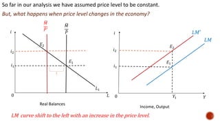
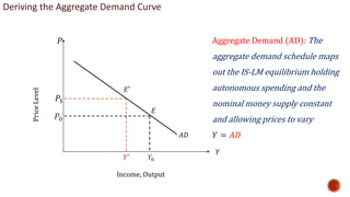
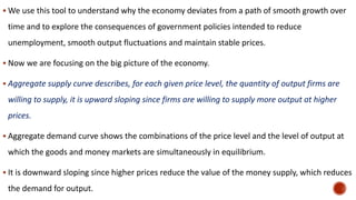
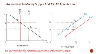
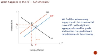
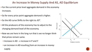
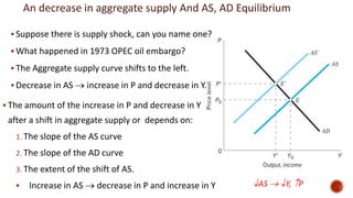
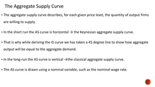
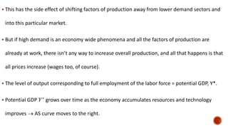
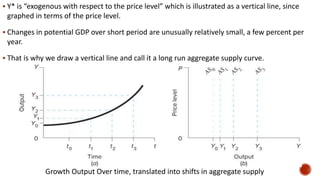
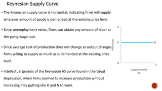
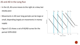
This document provides an overview of aggregate demand and aggregate supply concepts in macroeconomics. It defines key terms like aggregate demand curve, aggregate supply curve, equilibrium output and price level. It explains how shifts in aggregate demand and aggregate supply due to factors like money supply changes, government policies, supply shocks etc. affect equilibrium output and price level in both short-run and long-run. The document also discusses concepts like Keynesian and classical aggregate supply curves, supply-side economics and price adjustment mechanism.

1. AGGREGATE DEMAND AND
SUPPLY
Instructor: Dr. Amrita Kamalini Bhattacharyya
E-MAIL: ambhattacharyy@imt.edu
Mobile: 943293856
Institute Of Management Technology, Ghaziabad

2. So far in our analysis we have assumed price level to be constant.
But, what happens when price level changes in the economy?
𝑖
0 0 𝑌
𝐿
𝑖
𝐿1
𝑖2
𝑖1
𝑌1
Income, Output
𝑀
𝑃
Real Balances
𝐸1
𝐸2
𝐿𝑀
𝑀
𝑃′
𝐸1
𝐸2
𝐿𝑀′
𝑖1
𝑖2
𝐿𝑀 curve shift to the left with an increase in the price level.

3. Deriving the Aggregate Demand Curve
𝐴𝐷
𝑌
𝑃
𝐸
𝑃0
𝑌0
𝑌′
𝑃1
𝐸′
Income, Output
Price
Level
Aggregate Demand (AD): The
aggregate demand schedule maps
out the IS-LM equilibrium holding
autonomous spending and the
nominal money supply constant
and allowing prices to vary
𝑌 = 𝐴𝐷

4.  Macroeconomics is concerned with the behavior of the economy as a whole with booms and recessions,
the economy’s total output of goods and services, and the rates of inflation and unemployment.
 During Great Depression output of US fell by nearly 30%, between 1930 and 1940 the unemployment
rate averaged 18.8%.
 Unemployment rate of 2009 was 10%.
 During the great depression purchasing power of dollar rose by one-fourth.
 The AS/AD model is the basic macroeconomic tool for studying output fluctuations and the
determination of the price level and the inflation rate.
 This model is used to explain how the economy deviates from a path of smooth growth over time, and
to explore the consequences of government policies intended to reduce unemployment and output
fluctuations, and maintain stable price.

5.  We use this tool to understand why the economy deviates from a path of smooth growth over
time and to explore the consequences of government policies intended to reduce
unemployment, smooth output fluctuations and maintain stable prices.
 Now we are focusing on the big picture of the economy.
 Aggregate supply curve describes, for each given price level, the quantity of output firms are
willing to supply, it is upward sloping since firms are willing to supply more output at higher
prices.
 Aggregate demand curve shows the combinations of the price level and the level of output at
which the goods and money markets are simultaneously in equilibrium.
 It is downward sloping since higher prices reduce the value of the money supply, which reduces
the demand for output.

6. What we are here to learn and understand.
Suppose the RBI increases the money supply, what effect will that have on the
price level and on output?
Does increase in money supply lead to price level to rise, causing inflation?
Or does level of output rises?
Or do both inflation and output will rise?

7. AS, AD and Equilibrium
 AS and AD intersect at point E in Figure
 Equilibrium: AS = AD
 Equilibrium output is Y0 = observed level of
output in the economy at particular point in
time
 Equilibrium price level is P0 = observed price
level in the economy at particular point in
time

8. 𝑖
0 0 𝑌
𝐿
𝑖
𝐿1
𝑖2
𝑖1
𝑌1
Income, Output
𝑀′
𝑃
Real Balances
𝐸1
𝐸2
𝐿𝑀′
𝑀
𝑃
𝐸1
𝐸2
𝐿𝑀
𝑖1
𝑖2
𝐿𝑀 curve shift to the right with an increase in the money supply.
An Increase In Money Supply And AS, AD Equilibrium

9. What happens to the 𝐼𝑆 − 𝐿𝑀 schedule?
𝐿𝑀′
𝐼𝑆
𝑌
𝑖
𝐸
𝑖0
𝑌0
𝐸′
𝑌′
𝑖1
𝐿𝑀
Income, Output
Interest
Rate
We find that when money
supply rises in the economy LM
curve shift to the right and
aggregate demand for goods
and services rises and interest
rate decreases in the economy.

10. An Increase In Money Supply And AS, AD Equilibrium
 For the current price level aggregate demand in the economy
increases.
 So for every price point aggregate demand is higher.
 So the AD curve Shifts to the right to 𝐴𝐷′.
 All the producers of the economy has to adjust to the
changing demand level of the economy.
 Now we are here in the long run that is we no longer think
that prices remain same.
 Increase in AD  increase in P and Y
 an increase in AD resulting from an increase in money
supply.

11.  Thus an increase in the money stock causes both the level of output and the price level to rise.
 The amount of the increase in P and Y after a shift in aggregate demand depends on:
1. The slope of the AS curve
2. The slope of the AD curve
3. The extent of the shift of AD.
 Decrease in AD  decrease in P and Y
 Few things to remember, Price in microeconomics means the ratio at which two goods trade; in
contrast in macroeconomics price means the nominal price level, the cost of a basket of all the
goods we buy measured in money terms.

12.  Suppose there is supply shock, can you name one?
 What happened in 1973 OPEC oil embargo?
 The Aggregate supply curve shifts to the left.
 Decrease in AS  increase in P and decrease in Y.
 The amount of the increase in P and decrease in Y
after a shift in aggregate supply or depends on:
1. The slope of the AS curve
2. The slope of the AD curve
3. The extent of the shift of AS.
 Increase in AS  decrease in P and increase in Y
An decrease in aggregate supply And AS, AD Equilibrium
AS  Y, P

13. The Aggregate Supply Curve
 The aggregate supply curve describes, for each given price level, the quantity of output firms
are willing to supply.
 In the short run the AS curve is horizontal → the Keynesian aggregate supply curve.
 That is why while deriving the IS curve we has taken a 45 degree line to show how aggregate
output will be equal to the aggregate demand.
 In the long-run the AS curve is vertical →the classical aggregate supply curve.
 The AS curve is drawn using a nominal variable, such as the nominal wage rate.

14.  In the short-run, the nominal wage rate is fixed. As a result, an increasing price facilitated by an
increasing aggregate demand indicates higher profits that justify the expansion of output.
 When demand is continuously high, there are few production processes that have unemployed
fixed outputs. Any increase in demand production causes the prices to increase which results in
a steep or vertical AS curve.

15. Classical Supply Curve
 The classical supply curve is vertical, indicating that the same
amount of goods will be supplied, regardless of price.
 Based upon the assumption that the labor market is in equilibrium
with full employment of the labor force
 Remember, price level here means overall price level.
 In a single market manufacturers faced with high demand can raise
the price for their products and go out and buy more materials,
more labors and so forth.

16.  This has the side effect of shifting factors of production away from lower demand sectors and
into this particular market.
 But if high demand is an economy wide phenomena and all the factors of production are
already at work, there isn’t any way to increase overall production, and all that happens is that
all prices increase (wages too, of course).
 The level of output corresponding to full employment of the labor force = potential GDP, Y*.
 Potential GDP 𝑌∗
grows over time as the economy accumulates resources and technology
improves  AS curve moves to the right.

17.  Y* is “exogenous with respect to the price level” which is illustrated as a vertical line, since
graphed in terms of the price level.
 Changes in potential GDP over short period are unusually relatively small, a few percent per
year.
 That is why we draw a vertical line and call it a long run aggregate supply curve.
Growth Output Over time, translated into shifts in aggregate supply

18. Keynesian Supply Curve
 The Keynesian supply curve is horizontal, indicating firms will supply
whatever amount of goods is demanded at the existing price level.
 Since unemployment exists, firms can obtain any amount of labor at
the going wage rate.
 Since average cost of production does not change as output changes,
firms willing to supply as much as is demanded at the existing price
level.
 Intellectual genesis of the Keynesian AS curve found in the Great
Depression, when firms seemed to increase production without
increasing P by putting idle K and N to work.

19.  Additionally, prices are viewed as “sticky” in the short run. In the short run firms are reluctant
to change prices(and wages) when demand shifts.
 Instead at least for a while they increase or decrease output.
 As a result, aggregate supply curve is quite flat in the short run.
 In truth even in the very short run, the aggregate supply curve has a very slight upward tilt.

20. Frictional Unemployment or Natural Rate Of Unemployment
 Taken literally, the classical model implies that there is no involuntary unemployment 
everyone who wants to work is employed.
 In reality there is some unemployment due to frictions in the labor market (Ex. Someone is
always moving and looking for a new job).
 There will always be some frictional unemployment as people search for jobs.
 The unemployment rate associated with the full employment level of output that is known as
natural rate of unemployment.
 Natural rate of unemployment is the rate of unemployment arising from normal labor market
frictions that exist when the labor market is in equilibrium.

21. AD Curve And Shifts In AD
• AD shows the combination of the price level and level of output
at which the goods and money markets are simultaneously in
equilibrium.
• Expansionary policies such as increasing government spending,
cuts in taxes and increases in money supply move the aggregate
demand schedule to the right.
• Consumers and investors confidence also affects the aggregate
demand curve.
• Shifts in AD due to:
1. Policy measures (changes in G, T, and MS)
2. Consumer and investor confidence
Figure shows an increase in AD

22. AD Relationship Between Output And Prices
 Key to the AD relationship between output and prices is the dependency of AD on real money
supply.
 Real money supply = value of money provided by the central bank and the banking system.
 Real money supply is written as , where is the nominal money supply, and P is the price
level.
 For a given level of , high prices result in low OR high prices mean that the value of the
number of available dollars is low and thus a high P = low level of AD
P
M
M
M P
M
AD
I
r
P
M



 AD
I
r
P
M





23. AD Policy & The Keynesian Supply Curve
 AD schedule and the Keynesian aggregate supply schedule
 Initial equilibrium is at point E (AS = AD).
 At E goods and asset market are in equilibrium.
 Suppose an aggregate demand policy increases AD to AD’
this will shift the aggregate demand to the right, due to
increase in government spending or cut in taxes or increase
in money supply.
 The new equilibrium point, E’, corresponds to the same price
level, and a higher level of output (employment is also likely
to increase) cause firms are willing to supply any amount of
output at the level of prices 𝑃0, there is no effect in prices.

24. AD Policy & The Classical Supply Curve
 In the classical case, AS schedule is vertical at full employment
level of output.
 Firms will supply the level of output 𝑌∗
whatever the price level.
 The price level is not given, but depends upon the interaction
between AS and AD.
 The initial equilibrium point is E. Now a shift in AD schedule will
cause excess demand in the economy.
 When AD increases to AD’, spending increases to E’. But firms can
not obtain the labor required to meet the increased demand to
produce more output.

25. AD Policy & The Classical Supply Curve
 Firms hire more workers & wages and costs of production
rise  firms must charge higher price.
 Move up AS and AD curves to E’’ where AS = AD’
• Increase in demand then only increases prices not the
output level of the economy.
• Increase in prices reduces the real money stock and leads
to reduction in spending.
• Economy moves up AD’ schedule until prices have risen
enough and M/P has fallen enough to reduce spending to
a level consistent with full-employment output.
• This is when price level reaches 𝑃′
At point 𝐸′′ aggregate demand is once again
equal to aggregate supply only with higher
level of government spending.

26. Keynesian and Classical- Short run and Long run
 We have repeatedly used the term Keynesian and classical to describe assumptions of a horizontal or
vertical aggregate supply curve.
 Note that these are not alternative models providing alternative descriptions of the world.
 Both models are true: The Keynesian model holds in the short run, and the classical model holds in the
long run.
 Economists do have contentious disagreements over the time horizons in which either model applies.
 Almost all economists (almost all) agree that the Keynesian model holds over a period of a few months
or less and the classical model holds when the time frame is a decade or more.
 Unfortunately, the interesting time frame for policy relevance is several quarters to a few years.
 The speed with which prices adjust- that is, how long it takes the aggregate supply curve to rotate from
horizontal to vertical - is an area of active research.

27. SUPPLY SIDE ECONOMICS
 Supply side economics focuses on AS as the driver in the economy.
 Supply side policies are those that encourage growth in potential output  shift AS to right.
 Such policy measures include:
 Removing unnecessary regulation
 Maintaining efficient legal system
 Encouraging technological progress
 Politicians use the term supply side economics in reference to the idea that cutting taxes will
increase AS enough that tax collections will actually increase, rather than fall

28. Supply Side Economics
• Cutting tax rates has an impact on both AS and AD
–AD shifts to AD’ due to increase in disposable income
–Shift is relatively large compared to that of the AS
–AS shifts to AS’ as the incentive to work increases
• In short run, move to E’: GDP increases, tax revenues fall
proportionately less than tax cut (AD effect)
• In the LR, moves to E’’: GDP is higher, but by a small amount,
tax collections fall as the deficit rises, and prices rise (AS
effect)

29. Supply Side Economics
 Supply side policies are useful, despite previous example.
 Only supply side policies can permanently increase output.
 Demand side policies are useful for short run results
 Many economists support cutting taxes for the incentive effect, but with a simultaneous
reduction in government spending.
 Tax collections fall, but the reduction in government spending minimizes the impact on the
deficit

30. AS and AD in the Long Run
• In the LR, AS curve moves to the right at a slow, but
steady pace
• Movements in AD over long periods can be large or
small, depending largely on movements in money
supply
• Figure 5-12 shows a set of AS/AD curves for the
period 1970-2010

31. AS and the Price Adjustment Mechanism
 AS curve describes the price adjustment mechanism within the economy.
 The below figure shows the flat short-run aggregate supply curve in black and the vertical long
run curve in blue.
The dynamic
return to long
run aggregate
supply

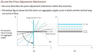
32.  It illustrates an entire spectrum of intermediate run curves.
 Think of aggregate supply curve is rotating counter
clockwise from horizontal to vertical with the passage of
time.
 The AS curve that applies say for 1-year horizon is a black
dashed line and medium sloped.
 If aggregate demand was higher than potential output 𝑌∗
then this black dashed line i.e. intermediate curve indicates
that after a year’s time prices will have risen enough to
partially , but not completely push GDP back down to
potential output.
 The figure on the left gives a static representation of a
dynamic process which is useful as well.
The AS curve is defined by the
equation:
where Pt-1 is the price level next
period, Pt is the price level today,
and Y* is potential output.
)]
(
1
[ *
1 Y
Y
P
P t
t 


 

33. )]
(
1
[ *
1 Y
Y
P
P t
t 


 
• What does the aggregate supply equation say?
• From the pure equation stand point it says, the price level of a period will depend on the price
level of previous period and how far the actual output of a country is from the potential
output.
• But what is the economic theory behind the idea?
• If output is above potential output , prices will rise and be higher next period; if prices are
below potential output, prices will fall and be lower next period.
• Prices will continue to rise or fall over time until output returns to potential output.
• The difference between actual GDP and potential GDP, 𝑌 − 𝑌∗
, is called GDP gap, or the
output gap.

34. AS And The Price Adjustment Mechanism
 Speed of the price adjustment mechanism controlled by 
 Policy implication: If  is large, the AS mechanism will return the economy to Y* relatively
quickly; if  is small, might want to use AD policy to speed up the adjustment process
)]
(
1
[ *
1 Y
Y
P
P t
t 


 

35. Let us summarize:
 A relatively flat aggregate supply curve means that changes in output and employment have a small
impact on prices.
 So a horizontal short-run AS curve moves up slowly in response to increases in output or employment.
 The coefficient 𝜆 captures this output/price linkages.
 The position of the short-run AS schedule depends on the level of prices. The schedule passes through
the full-employment level of output, 𝑌∗
, at 𝑃𝑡+1 = 𝑃𝑡.
 At higher output levels there is overemployment, hence prices next period will be higher than those this
period.
 The short run As shifts over time. If output is maintained above the full employment level, 𝑌∗
prices will
continue to rise over time.

36. THANK
YOU