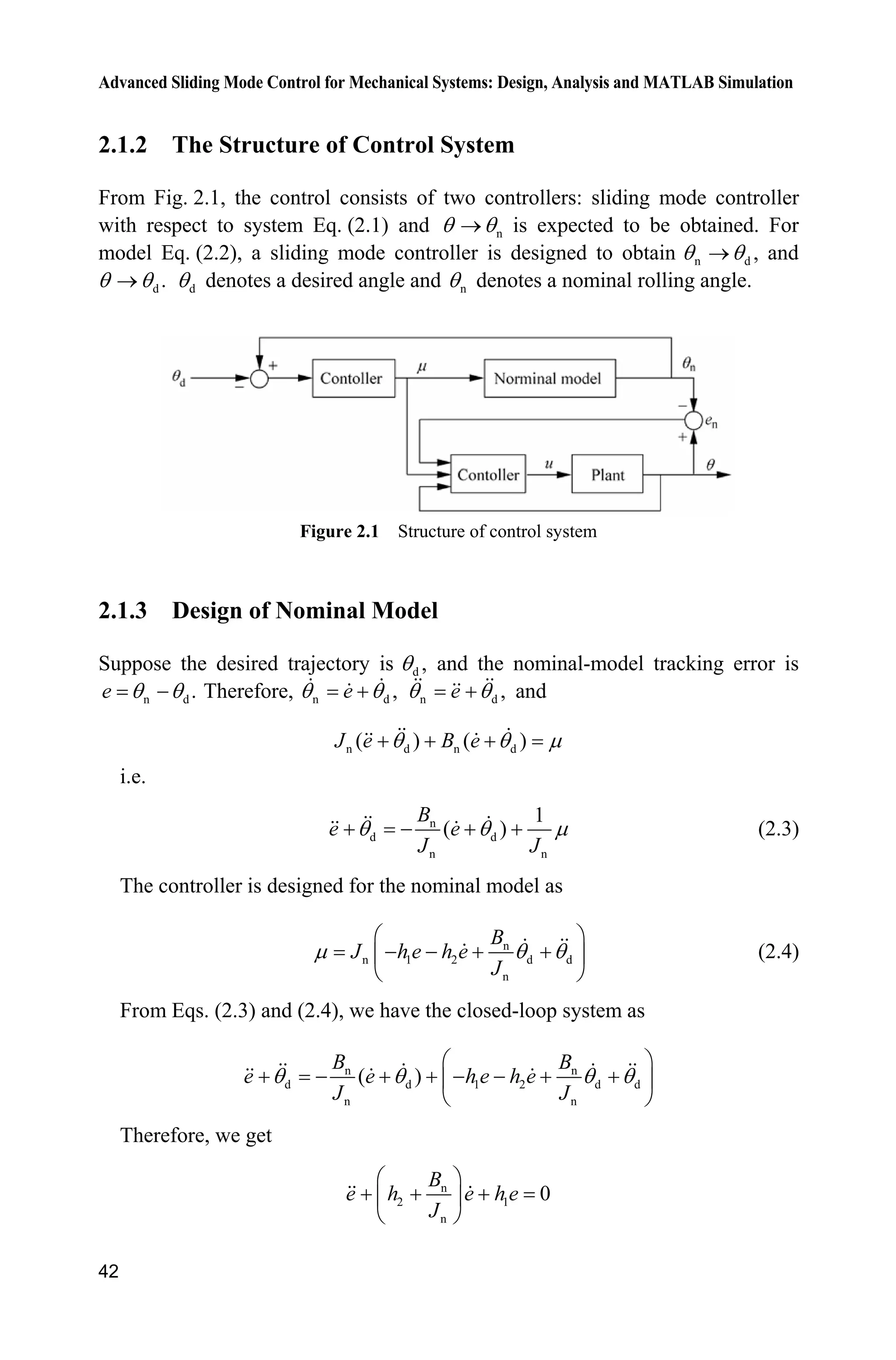
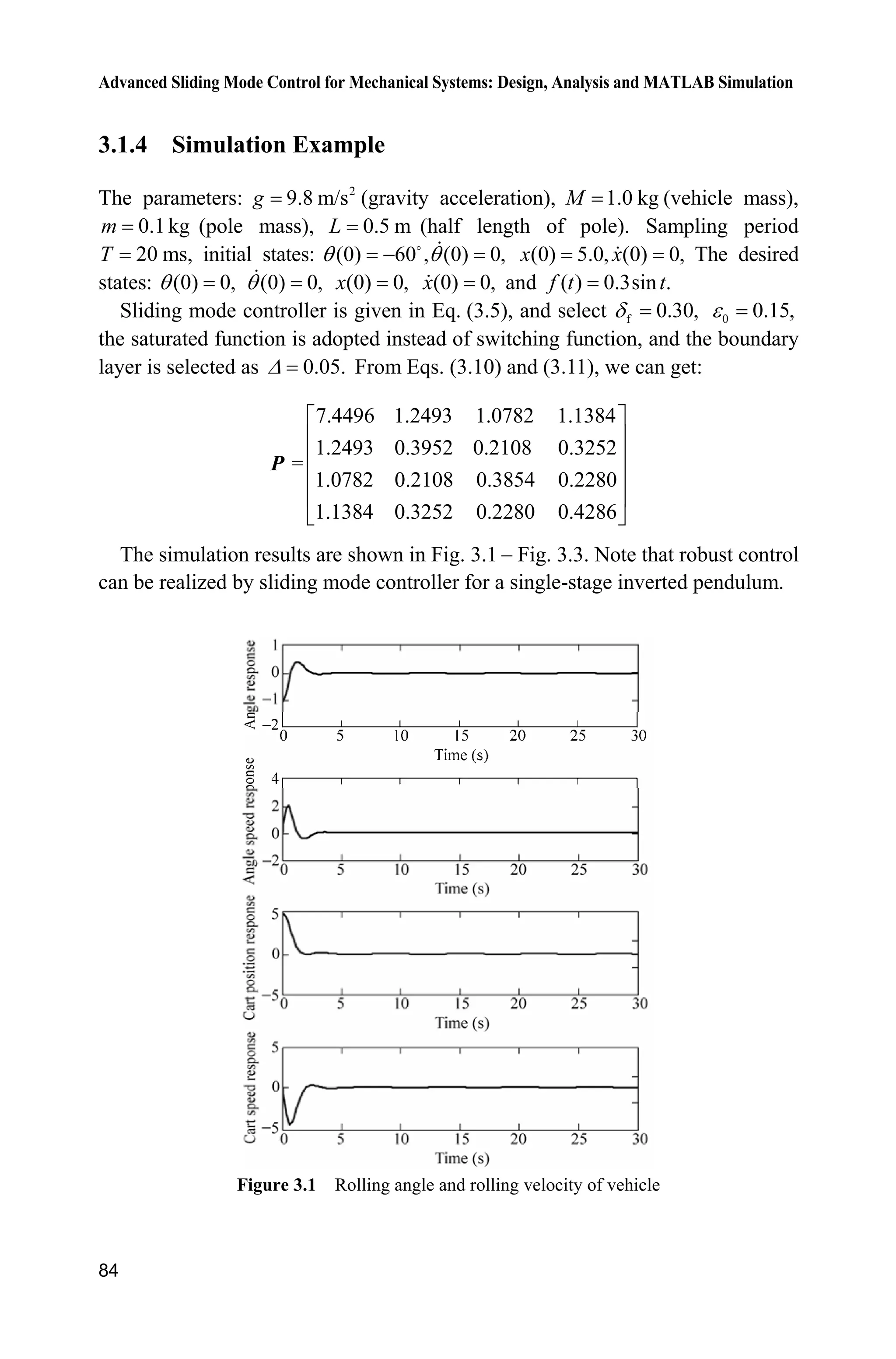
This document provides an overview and table of contents for a book on advanced sliding mode control for mechanical systems. The book covers topics such as sliding mode controller design, analysis, and MATLAB simulation. It includes 11 chapters that discuss various sliding mode control approaches, such as normal sliding mode control, advanced sliding mode control, discrete sliding mode control, adaptive sliding mode control, terminal sliding mode control, and sliding mode control based on observers. Case studies and MATLAB programs are provided to illustrate practical applications of the theory.
![1 Introduction
Jinkun Liu
Beijing University of Aeronautics and Astronautics
P.R.China
E-mail: ljk@buaa.edu.cn
Xinhua Wang
National University of Singapore
Singapore
E-mail: wangxinhua04@gmail.com
Abstract This chapter introduces the concept of sliding mode control and
illustrates the attendant features of robustness and performance specification
using a straightforward example, several typical sliding mode controllers for
continuous system are given, a concrete stability analysis, simulation examples
and Matlab programs are given too.
Keywords sliding mode control, sliding surface, Reaching Law, quasi-sliding
mode, equivalent control
One of the methods used to solve control problems are the sliding mode techniques.
These techniques are generating greater interest.
This book provides the reader with an introduction to classical sliding mode
control design examples. Fully worked design examples, which can be used as
tutorial material, are included. Industrial case studies, which present the results of
sliding mode controller implementations, are used to illustrate successful practical
applications of the theory.
Typically, discrepancies may occur between the actual plant and the mathematical
model developed for the controller design. These mismatches may be due to various
factors. The engineer’s role is to ensure required performance levels despite such
mismatches. A set of robust control methods have been developed to eliminate any
discrepancy. One such approach to the robust control controller design is called
the sliding mode control (SMC) methodology. This is a specific type of variable
structure control system (VSCS).
In the early 1950s, Emelyanov and several co-researchers such as Utkins and
Itkis[1]
from the Soviet Union, proposed and elaborated the variable structure control
Advanced Sliding Mode Control for Mechanical Systems
© Tsinghua University Press, Beijing and Springer-Verlag Berlin Heidelberg 201
J. Liu et al.,
2](https://image.slidesharecdn.com/advancedslidingmodecontrolformechanicalsystems-130611121131-phpapp01/75/Advanced-sliding-mode-control-for-mechanical-systems-15-2048.jpg)
![Advanced Sliding Mode Control for Mechanical Systems: Design, Analysis and MATLAB Simulation
2
(VSC) with sliding mode control. During the past decades, VSC and SMC have
generated significant interest in the control research community.
SMC has been applied into general design method being examined for wide
spectrum of system types including nonlinear system, multi-input multi-output
(MIMO) systems, discrete-time models, large-scale and infinite-dimension systems,
and stochastic systems. The most eminent feature of SMC is it is completely
insensitive to parametric uncertainty and external disturbances during sliding
mode[2]
.
VSC utilizes a high-speed switching control law to achieve two objectives.
Firstly, it drives the nonlinear plant’s state trajectory onto a specified and user-
chosen surface in the state space which is called the sliding or switching surface.
This surface is called the switching surface because a control path has one gain if
the state trajectory of the plant is “above” the surface and a different gain if the
trajectory drops “below” the surface. Secondly, it maintains the plant’s state
trajectory on this surface for all subsequent times. During the process, the control
system’s structure varies from one to another and thereby earning the name
variable structure control. The control is also called as the sliding mode control[3]
to emphasize the importance of the sliding mode.
Under sliding mode control, the system is designed to drive and then constrain
the system state to lie within a neighborhood of the switching function. Its two
main advantages are (1) the dynamic behavior of the system may be tailored by
the particular choice of switching function, and (2) the closed-loop response
becomes totally insensitive to a particular class of uncertainty. Also, the ability to
specify performance directly makes sliding mode control attractive from the
design perspective.
Trajectory of a system can be stabilized by a sliding mode controller. The
system states “slides” along the line 0s after the initial reaching phase. The
particular 0s surface is chosen because it has desirable reduced-order dynamics
when constrained to it. In this case, the 1 1,s cx x 0c ! surface corresponds to
the first-order LTI system 1 1,x cx which has an exponentially stable origin. Now,
we consider a simple example of the sliding mode controller design as under.
Consider a plant as
( ) ( )J t u tT (1.1)
where J is the inertia moment, ( )tT is the angle signal, and ( )u t is the control
input.
Firstly, we design the sliding mode function as
( ) ( ) ( )s t ce t e t (1.2)
where c must satisfy the Hurwitz condition, 0.c !
The tracking error and its derivative value are
d( ) ( ) ( ),e t t tT T d( ) ( ) ( )e t t tT T](https://image.slidesharecdn.com/advancedslidingmodecontrolformechanicalsystems-130611121131-phpapp01/75/Advanced-sliding-mode-control-for-mechanical-systems-16-2048.jpg)
![1 Introduction
3
where ( )tT is the practical position signal, and d ( )tT is the ideal position signal.
Therefore, we have
d d
1
( ) ( ) ( ) ( ) ( ) ( ) ( ) ( )s t ce t e t ce t t t ce t u t
J
T T T (1.3)
and
d
1
ss s ce u
J
T
§ ·
¨ ¸
© ¹
Secondly, to satisfy the condition 0,ss we design the sliding mode controller as
d( ) ( sgn( )),u t J ce sT K
1, 0
sgn( ) 0, 0
1, 0
s
s s
s
!
°
®
° ¯
(1.4)
Then, we get
| | 0ss sK
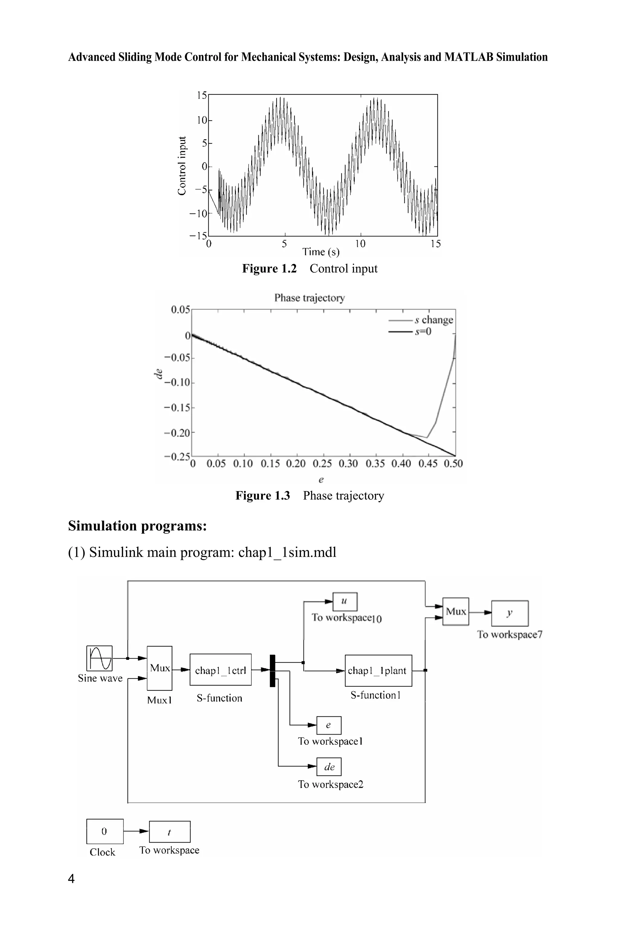
A simulation example is presented for explanation. Consider the plant as
( ) ( )J t u tT
where 10.J
The initial state is set as [0.5 1.0] after choosing the position ideal signal
d ( ) sin .t tT Using controller Eq. (1.4) wherein 0.5,c 0.5K the results are
derived as shown in Fig. 1.1 Fig. 1.3.
Figure 1.1 Position and speed tracking](https://image.slidesharecdn.com/advancedslidingmodecontrolformechanicalsystems-130611121131-phpapp01/75/Advanced-sliding-mode-control-for-mechanical-systems-17-2048.jpg)
![1 Introduction
5
(2) Controller: chap1_1ctrl.m
function [sys,x0,str,ts] = spacemodel(t,x,u,flag)
switch flag,
case 0,
[sys,x0,str,ts]=mdlInitializeSizes;
case 3,
sys=mdlOutputs(t,x,u);
case {2,4,9}
sys=[];
otherwise
error(['Unhandled flag = ',num2str(flag)]);
end
function [sys,x0,str,ts]=mdlInitializeSizes
sizes = simsizes;
sizes.NumContStates = 0;
sizes.NumDiscStates = 0;
sizes.NumOutputs = 3;
sizes.NumInputs = 3;
sizes.DirFeedthrough = 1;
sizes.NumSampleTimes = 0;
sys = simsizes(sizes);
x0 = [];
str = [];
ts = [];
function sys=mdlOutputs(t,x,u)
thd=u(1);
dthd=cos(t);
ddthd=-sin(t);
th=u(2);
dth=u(3);
c=0.5;
e=th-thd;
de=dth-dthd;
s=c*e+de;
J=10;
xite=0.50;
ut=J*(-c*de+ddthd-xite*sign(s));
sys(1)=ut;
sys(2)=e;
sys(3)=de;
(3) Plant: chap1_1plant.m
function [sys,x0,str,ts]=s_function(t,x,u,flag)
switch flag,
case 0,
[sys,x0,str,ts]=mdlInitializeSizes;
case 1,](https://image.slidesharecdn.com/advancedslidingmodecontrolformechanicalsystems-130611121131-phpapp01/75/Advanced-sliding-mode-control-for-mechanical-systems-19-2048.jpg)
![Advanced Sliding Mode Control for Mechanical Systems: Design, Analysis and MATLAB Simulation
6
sys=mdlDerivatives(t,x,u);
case 3,
sys=mdlOutputs(t,x,u);
case {2, 4, 9 }
sys = [];
otherwise
error(['Unhandled flag = ',num2str(flag)]);
end
function [sys,x0,str,ts]=mdlInitializeSizes
sizes = simsizes;
sizes.NumContStates = 2;
sizes.NumDiscStates = 0;
sizes.NumOutputs = 2;
sizes.NumInputs = 1;
sizes.DirFeedthrough = 0;
sizes.NumSampleTimes = 0;
sys=simsizes(sizes);
x0=[0.5 1.0];
str=[];
ts=[];
function sys=mdlDerivatives(t,x,u)
J=10;
sys(1)=x(2);
sys(2)=1/J*u;
function sys=mdlOutputs(t,x,u)
sys(1)=x(1);
sys(2)=x(2);
(4) Plot program: chap1_1plot.m
close all;
figure(1);
subplot(211);
plot(t,y(:,1),'k',t,y(:,2),'r:','linewidth',2);
legend('Ideal position signal','Position tracking');
xlabel('time(s)');ylabel('Angle response');
subplot(212);
plot(t,cos(t),'k',t,y(:,3),'r:','linewidth',2);
legend('Ideal speed signal','Speed tracking');
xlabel('time(s)');ylabel('Angle speed response');
figure(2);
plot(t,u(:,1),'k','linewidth',0.01);
xlabel('time(s)');ylabel('Control input');
c=0.5;
figure(3);
plot(e,de,'r',e,-c'.*e,'k','linewidth',2);
xlabel('e');ylabel('de');
legend('s change','s=0');
title( phase trajectory');](https://image.slidesharecdn.com/advancedslidingmodecontrolformechanicalsystems-130611121131-phpapp01/75/Advanced-sliding-mode-control-for-mechanical-systems-20-2048.jpg)
![1 Introduction
7
Sliding mode control is a nonlinear control method that alters the dynamics of
a nonlinear system by the multiple control structures are designed so as to ensure
that trajectories always move towards a switching condition. Therefore, the ultimate
trajectory will not exist entirely within one control structure. The state-feedback
control law is not a continuous function of time. Instead, it switches from one
continuous structure to another based on the current position in the state space.
Hence, sliding mode control is a variable structure control method. The multiple
control structures are designed so as to ensure that trajectories always move
towards a switching condition. Therefore, the ultimate trajectory will not exist
entirely within one control structure. Instead, the ultimate trajectory will slide
along the boundaries of the control structures. The motion of the system as it
slides along these boundaries is called a sliding mode[3]
and the geometrical locus
consisting of the boundaries is called the sliding (hyper) surface. Figure 1.3 shows
an example of the trajectory of a system under sliding mode control. The sliding
surface is described by s 0, and the sliding mode along the surface commences
after the finite time when system trajectories have reached the surface. In the
context of modern control theory, any variable structure system like a system
under SMC, may be viewed as a special case of a hybrid dynamical system.
Intuitively, sliding mode control uses practically infinite gain to force the
trajectories of a dynamic system to slide along the restricted sliding mode
subspace. Trajectories from this reduced-order sliding mode have desirable
properties (e.g., the system naturally slides along it until it comes to rest at a
desired equilibrium). The main strength of sliding mode control is its robustness.
Because the control can be as simple as a switching between two states, it need
not be precise and will not be sensitive to parameter variations that enter into the
control channel. Additionally, because the control law is not a continuous function,
the sliding mode can be reached in finite time (i.e., better than asymptotic behavior).
There are two steps in the SMC design. The first step is designing a sliding
surface so that the plant restricted to the sliding surface has a desired system
response. This means the state variables of the plant dynamics are constrained to
satisfy another set of equations which define the so-called switching surface. The
second step is constructing a switched feedback gains necessary to drive the
plant’s state trajectory to the sliding surface. These constructions are built on the
generalized Lyapunov stability theory.
1.1 Parameters of Sliding Surface Design
For linear system
, ,n
u u x Ax b x R R (1.5)
where x is system state, A is an nun matrix, b is an nu1 vector, and u is control
input. A sliding variable can be designed as](https://image.slidesharecdn.com/advancedslidingmodecontrolformechanicalsystems-130611121131-phpapp01/75/Advanced-sliding-mode-control-for-mechanical-systems-21-2048.jpg)
![Advanced Sliding Mode Control for Mechanical Systems: Design, Analysis and MATLAB Simulation
8
1
T
1 1
( )
n n
i i i i n
i i
c x c x x
¦ ¦s x C x (1.6)
where x is state vector, T
1 1[ 1] .nc c C
In sliding mode control, parameters 1 2 1, , , nc c c should be selected so that
the polynomial 1 2
1 2 1
n n
np c p c p c
is a Hurwitz polynomial, where p
is a Laplace operator.
For example, 2,n 1 1 2( ) ,c x xs x to satisfy the condition that the polynomial
1p c is Hurwitz, the eigenvalue of 1 0p c should have a negative real part,
i.e. 1 0.c !
Consider another example, 3,n 1 1 2 2 3( ) ,c x c x x s x to satisfy the condition
that the polynomial 2
2 1p c p c is Hurwitz, the eigenvalue of 2
2p c p 1 0c
should have a negative real part. For a positive constant O in 2
( ) 0,p O we
can get 2 2
2 0.p pO O Therefore, we have 2 2 ,c O 2
1 .c O
1.2 Sliding Mode Control Based on Reaching Law
Sliding mode based on reaching law includes reaching phase and sliding phase.
The reaching phase drive system is to maintain a stable manifold and the sliding
phase drive system ensures slide to equilibrium. The idea of sliding mode can be
described as Fig. 1.4.
Figure 1.4 The idea of sliding mode
1.2.1 Classical Reaching Laws
(1) Constant Rate Reaching Law
sgn( ), 0s sH H ! (1.7)](https://image.slidesharecdn.com/advancedslidingmodecontrolformechanicalsystems-130611121131-phpapp01/75/Advanced-sliding-mode-control-for-mechanical-systems-22-2048.jpg)
![Advanced Sliding Mode Control for Mechanical Systems: Design, Analysis and MATLAB Simulation
10
Therefore, we have
( ) ( ) ( ) ( ( )) ( ( ))
( ( )) ( ( , ) ( ))
s t ce t e t c r t r t
c r t r f t bu t
T T
T T
(1.13)
According to the exponential reaching law, we have
sgn , 0, 0s s ks kH H ! ! (1.14)
From Eqs. (1.13) and (1.14), we have
( ( )) ( ( , ) ( )) sgnc r t r f t bu t s ksT T H
Then we can get the sliding mode controller as
1
( ) ( sgn( ) ( ( )) ( , ))u t s ks c r t r f t
b
H T T (1.15)
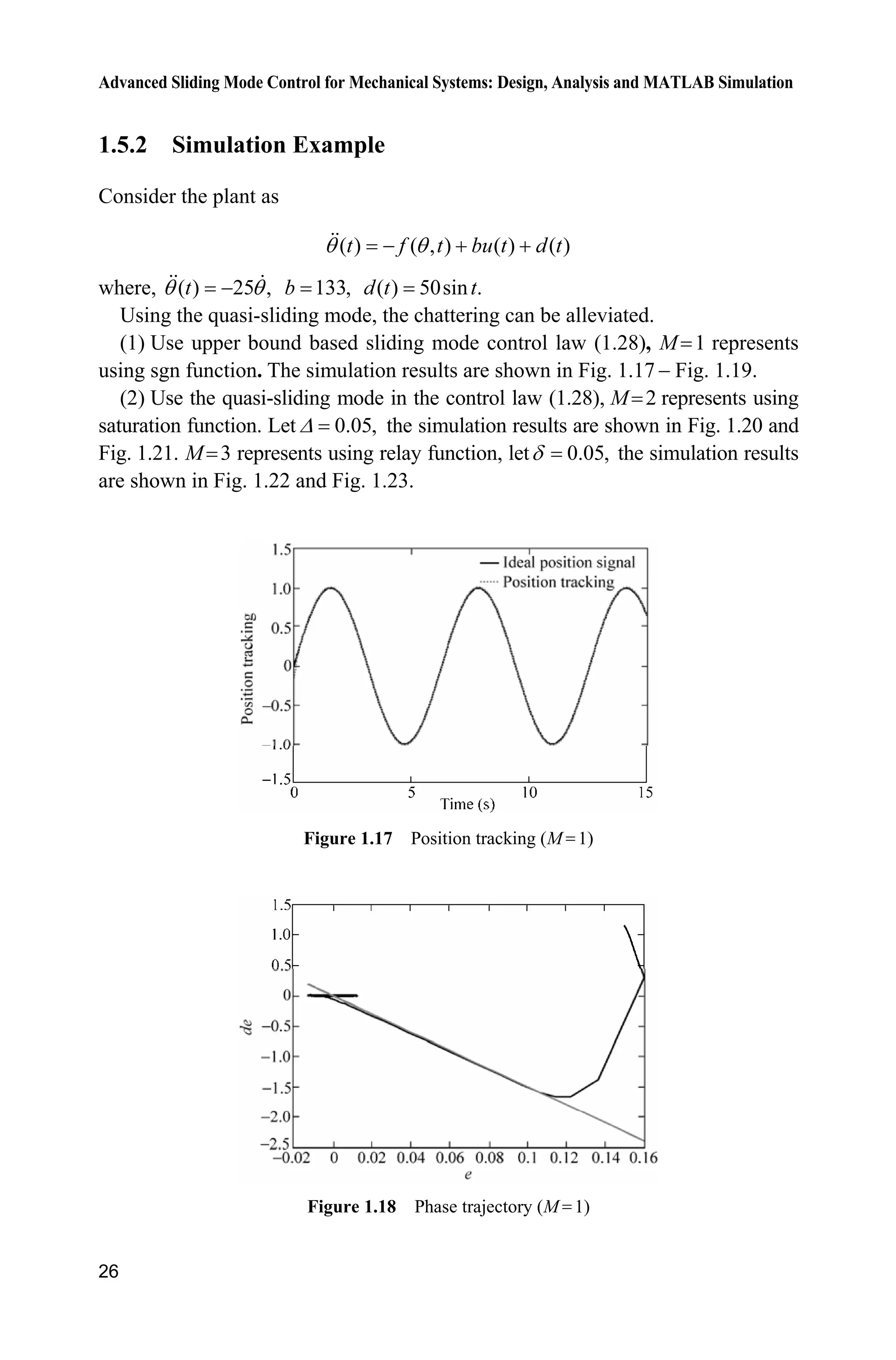
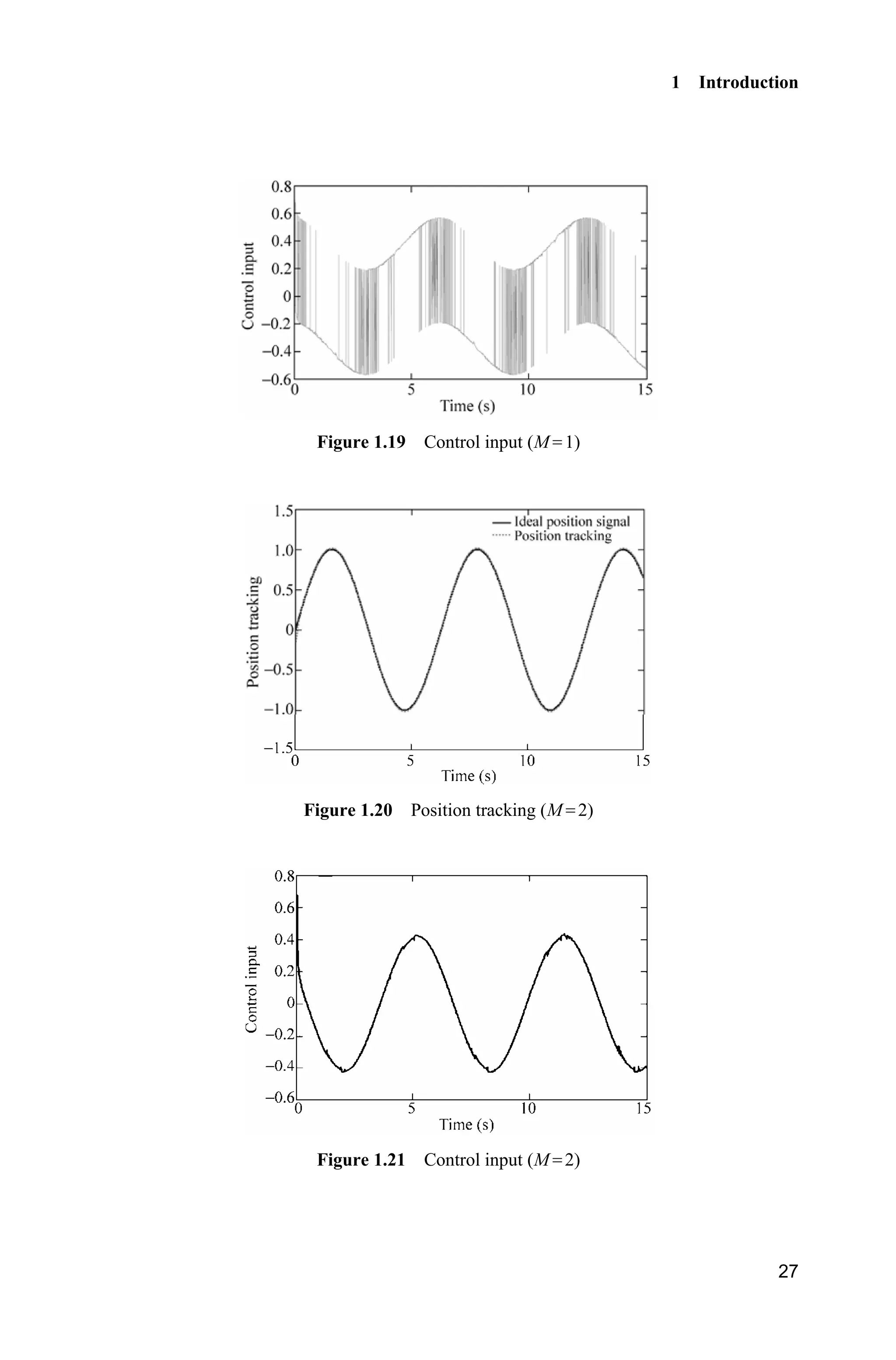
1.2.2.2 Simulation Example
Consider the plant as
( ) ( , ) ( )t f t bu tT T
where ( ) 25 ,tT T 133b .
Choosing position ideal signal ( ) sin ,r t t the initial state is set as
[ 0.15 0.15], using controller Eq. (1.15), 15,c 5,H 10,k the results
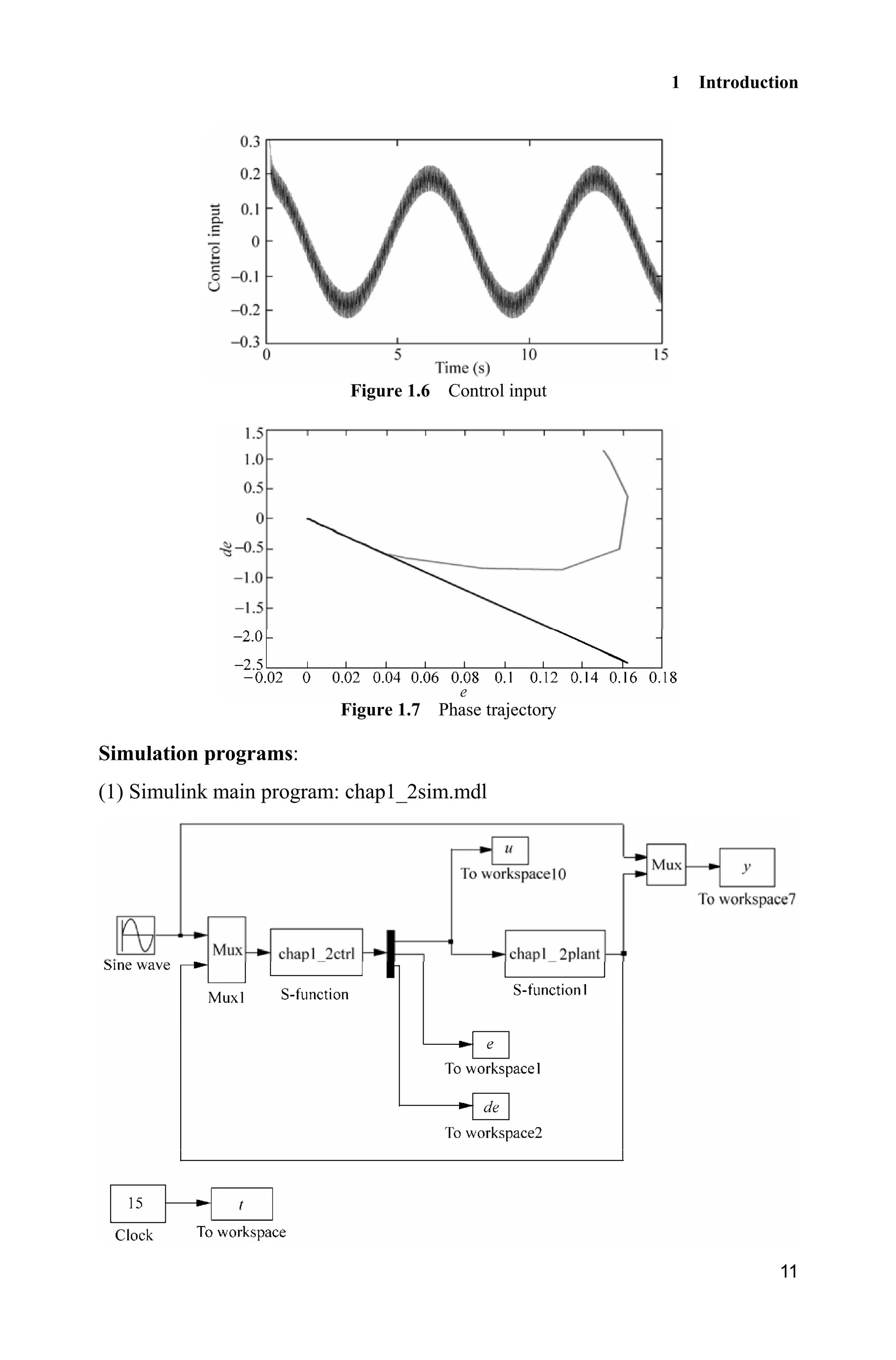
can be seen in Fig. 1.5 Fig. 1.7.
Figure 1.5 Position tracking](https://image.slidesharecdn.com/advancedslidingmodecontrolformechanicalsystems-130611121131-phpapp01/75/Advanced-sliding-mode-control-for-mechanical-systems-24-2048.jpg)
![Advanced Sliding Mode Control for Mechanical Systems: Design, Analysis and MATLAB Simulation
12
(2) Controller: chap1_2ctrl.m
function [sys,x0,str,ts] = spacemodel(t,x,u,flag)
switch flag,
case 0,
[sys,x0,str,ts]=mdlInitializeSizes;
case 3,
sys=mdlOutputs(t,x,u);
case {2,4,9}
sys=[];
otherwise
error(['Unhandled flag = ',num2str(flag)]);
end
function [sys,x0,str,ts]=mdlInitializeSizes
sizes = simsizes;
sizes.NumContStates = 0;
sizes.NumDiscStates = 0;
sizes.NumOutputs = 3;
sizes.NumInputs = 3;
sizes.DirFeedthrough = 1;
sizes.NumSampleTimes = 0;
sys = simsizes(sizes);
x0 = [];
str = [];
ts = [];
function sys=mdlOutputs(t,x,u)
r=u(1);
dr=cos(t);
ddr=-sin(t);
th=u(2);
dth=u(3);
c=15;
e=r-th;
de=dr-dth;
s=c*e+de;
fx=25*dth;
b=133;
epc=5;k=10;
ut=1/b*(epc*sign(s)+k*s+c*de+ddr+fx);
sys(1)=ut;
sys(2)=e;
sys(3)=de;
(3) Plant: chap1_2plant.m
function [sys,x0,str,ts]=s_function(t,x,u,flag)](https://image.slidesharecdn.com/advancedslidingmodecontrolformechanicalsystems-130611121131-phpapp01/75/Advanced-sliding-mode-control-for-mechanical-systems-26-2048.jpg)
![1 Introduction
13
switch flag,
case 0,
[sys,x0,str,ts]=mdlInitializeSizes;
case 1,
sys=mdlDerivatives(t,x,u);
case 3,
sys=mdlOutputs(t,x,u);
case {2, 4, 9 }
sys = [];
otherwise
error(['Unhandled flag = ',num2str(flag)]);
end
function [sys,x0,str,ts]=mdlInitializeSizes
sizes = simsizes;
sizes.NumContStates = 2;
sizes.NumDiscStates = 0;
sizes.NumOutputs = 2;
sizes.NumInputs = 1;
sizes.DirFeedthrough = 0;
sizes.NumSampleTimes = 0;
sys=simsizes(sizes);
x0=[-0.15 -0.15];
str=[];
ts=[];
function sys=mdlDerivatives(t,x,u)
sys(1)=x(2);
sys(2)=-25*x(2)+133*u;
function sys=mdlOutputs(t,x,u)
sys(1)=x(1);
sys(2)=x(2);
(4) Plot program: chap1_2plot.m
close all;
figure(1);
plot(t,y(:,1),'k',t,y(:,2),'r:','linewidth',2);
legend('Ideal position signal','Position tracking');
xlabel('time(s)');ylabel('Angle response');
figure(2);
plot(t,u(:,1),'k','linewidth',0.01);
xlabel('time(s)');ylabel('Control input');
c=15;
figure(3);
plot(e,de,'r',e,-c'.*e,'k','linewidth',2);
xlabel('e');ylabel('de');](https://image.slidesharecdn.com/advancedslidingmodecontrolformechanicalsystems-130611121131-phpapp01/75/Advanced-sliding-mode-control-for-mechanical-systems-27-2048.jpg)
![1 Introduction
15
where, cd is chosen to guarantee the reaching condition.
Substituting Eq. (1.21) into Eq. (1.18) and simplifying the result, we get
c( ) sgn( )s t s ks d dH (1.22)
The term cd can be chosen to ensure the reaching condition. It is reasonable to
assume that d is bounded, therefore, so is c.d That is
L U( )d d t d (1.23)
where the bounds Ld and Ud are known.
Referring to Eq. (1.22), cd is chosen according to the following logic;
When ( ) 0,s t ! c( ) ,s t ks d dH we want ( ) 0,s t so let c Ld d
When ( ) 0,s t c( ) ,s t ks d dH we want ( ) 0,s t ! so let c Ud d
Therefore, if we define U L
1 ,
2
d d
d
U L
2 ,
2
d d
d
then we can get
c 2 1 sgn( )d d d s (1.24)
1.3.2 Simulation Example
Consider the plant as
( ) ( , ) ( ) ( )t f t bu t d tT T
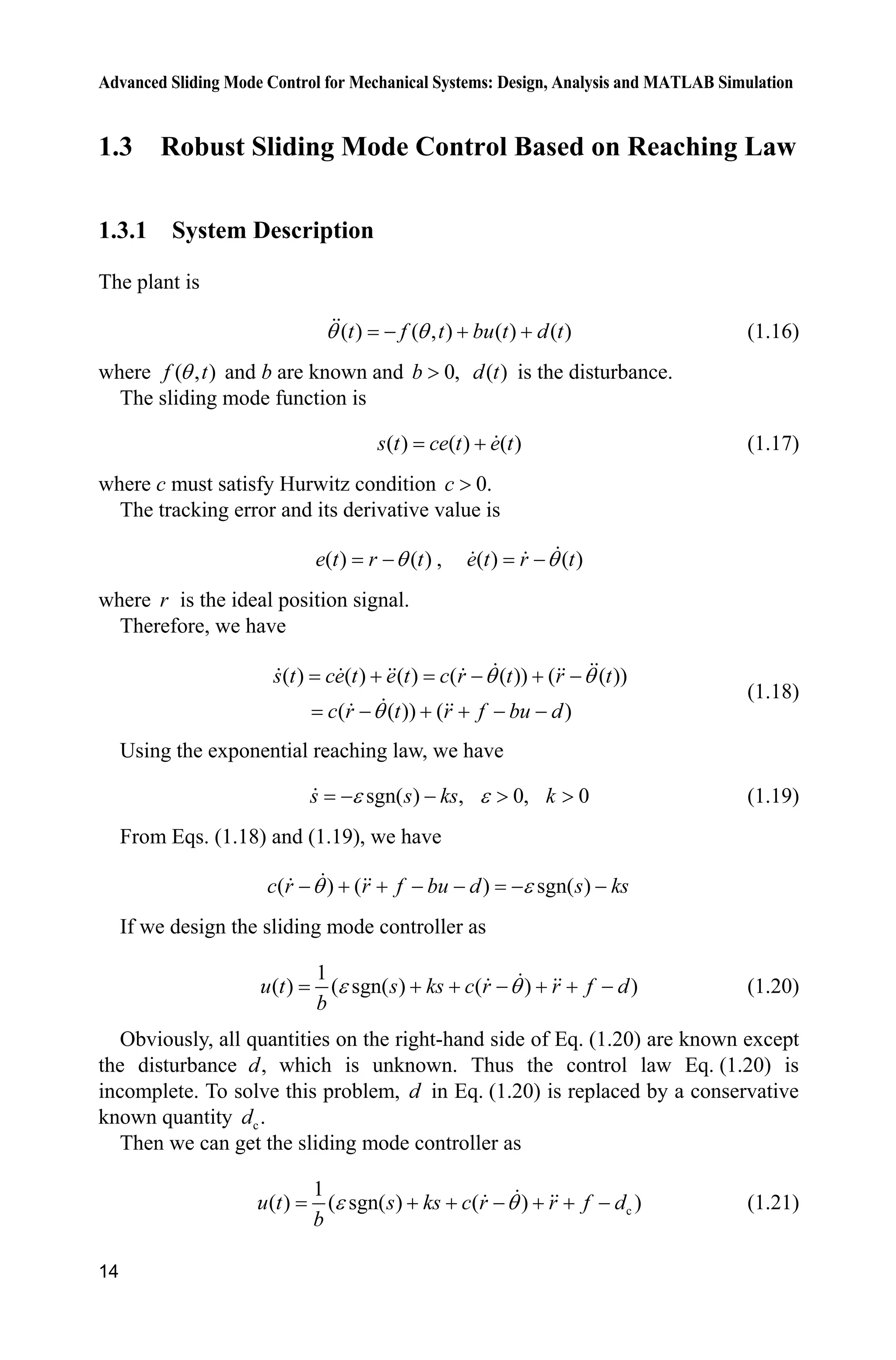
where ( ) 25 ,tT T 133,b ( ) 10sin ( ).d t tS
Choosing position ideal signal ( ) sin ,r t t the initial state is set as
[ 0.15 0.15], using controller Eq. (1.21), 15,c 0.5,H 10,k the results
can be seen in Fig. 1.8 Fig. 1.10.
Figure 1.8 Position tracking](https://image.slidesharecdn.com/advancedslidingmodecontrolformechanicalsystems-130611121131-phpapp01/75/Advanced-sliding-mode-control-for-mechanical-systems-29-2048.jpg)
![1 Introduction
17
(2) Controller: chap1_3ctrl.m
function [sys,x0,str,ts] = spacemodel(t,x,u,flag)
switch flag,
case 0,
[sys,x0,str,ts]=mdlInitializeSizes;
case 3,
sys=mdlOutputs(t,x,u);
case {2,4,9}
sys=[];
otherwise
error(['Unhandled flag = ',num2str(flag)]);
end
function [sys,x0,str,ts]=mdlInitializeSizes
sizes = simsizes;
sizes.NumContStates = 0;
sizes.NumDiscStates = 0;
sizes.NumOutputs = 3;
sizes.NumInputs = 3;
sizes.DirFeedthrough = 1;
sizes.NumSampleTimes = 0;
sys = simsizes(sizes);
x0 = [];
str = [];
ts = [];
function sys=mdlOutputs(t,x,u)
r=u(1);
dr=cos(t);
ddr=-sin(t);
th=u(2);
dth=u(3);
c=15;
e=r-th;
de=dr-dth;
s=c*e+de;
fx=25*dth;
b=133;
dL=-10;dU=10;
d1=(dU-dL)/2;
d2=(dU+dL)/2;
dc=d2-d1*sign(s);
epc=0.5;k=10;
ut=1/b*(epc*sign(s)+k*s+c*de+ddr+fx-dc);
sys(1)=ut;
sys(2)=e;
sys(3)=de;](https://image.slidesharecdn.com/advancedslidingmodecontrolformechanicalsystems-130611121131-phpapp01/75/Advanced-sliding-mode-control-for-mechanical-systems-31-2048.jpg)
![Advanced Sliding Mode Control for Mechanical Systems: Design, Analysis and MATLAB Simulation
18
(3) Plant: chap1_3plant.m
function [sys,x0,str,ts]=s_function(t,x,u,flag)
switch flag,
case 0,
[sys,x0,str,ts]=mdlInitializeSizes;
case 1,
sys=mdlDerivatives(t,x,u);
case 3,
sys=mdlOutputs(t,x,u);
case {2, 4, 9 }
sys = [];
otherwise
error(['Unhandled flag = ',num2str(flag)]);
end
function [sys,x0,str,ts]=mdlInitializeSizes
sizes = simsizes;
sizes.NumContStates = 2;
sizes.NumDiscStates = 0;
sizes.NumOutputs = 2;
sizes.NumInputs = 1;
sizes.DirFeedthrough = 0;
sizes.NumSampleTimes = 0;
sys=simsizes(sizes);
x0=[-0.15 -0.15];
str=[];
ts=[];
function sys=mdlDerivatives(t,x,u)
sys(1)=x(2);
sys(2)=-25*x(2)+133*u+10*sin(pi*t);
function sys=mdlOutputs(t,x,u)
sys(1)=x(1);
sys(2)=x(2);
(4) Plot program: chap1_3plot.m
close all;
figure(1);
plot(t,y(:,1),'k',t,y(:,2),'r:','linewidth',2);
legend('Ideal position signal','Position tracking');
xlabel('time(s)');ylabel('Position tracking');
figure(2);
plot(t,u(:,1),'k','linewidth',2);
xlabel('time(s)');ylabel('Control input');
c=15;
figure(3);
plot(e,de,'k',e,-c'.*e,'r','linewidth',2);
xlabel('e');ylabel('de');](https://image.slidesharecdn.com/advancedslidingmodecontrolformechanicalsystems-130611121131-phpapp01/75/Advanced-sliding-mode-control-for-mechanical-systems-32-2048.jpg)
![1 Introduction
19
1.4 Sliding Mode Robust Control Based on Upper Bound
1.4.1 System Description
Consider a second-order nonlinear inverted pendulum as follows:
0( , ) ( , ) ( , ) ( , ) ( )f f g u g u d tT T T T T T T T T ' ' (1.25)
where f and g are known nonlinear functions, u R and y RT are the
control input and measurement output respectively. 0 ( )d t is the disturbance, and
| ( , , ) | ,d t DT T D is a positive constant.
Let 0( , , ) ( , ) ( , ) ( ),d t f g u d tT T T T T T' ' therefore, Eq. (1.25) can be written
as
( , ) ( , ) ( , , )f g u d tT T T T T T T (1.26)
1.4.2 Controller Design
Let desired position input be d ,T and d .e T T The sliding variable is selected as
s = e+ce (1.27)
where 0.c ! Therefore,
d ds e +ce ce f gu d ceT T T
The controller is adopted as
d
1
[ sgn( )]u f ce s
g
T K (1.28)
elect the Lyapunov function as
21
2
L s
Therefore, we have
d
d d
( )
( ( sgn( )) )
( sgn ( ))
| |
L ss s f gu d ce
s f f ce s d ce
s d s
sd s
T
T T K
K
K
If ,DK then
| | 0L sd sK](https://image.slidesharecdn.com/advancedslidingmodecontrolformechanicalsystems-130611121131-phpapp01/75/Advanced-sliding-mode-control-for-mechanical-systems-33-2048.jpg)
![Advanced Sliding Mode Control for Mechanical Systems: Design, Analysis and MATLAB Simulation
20
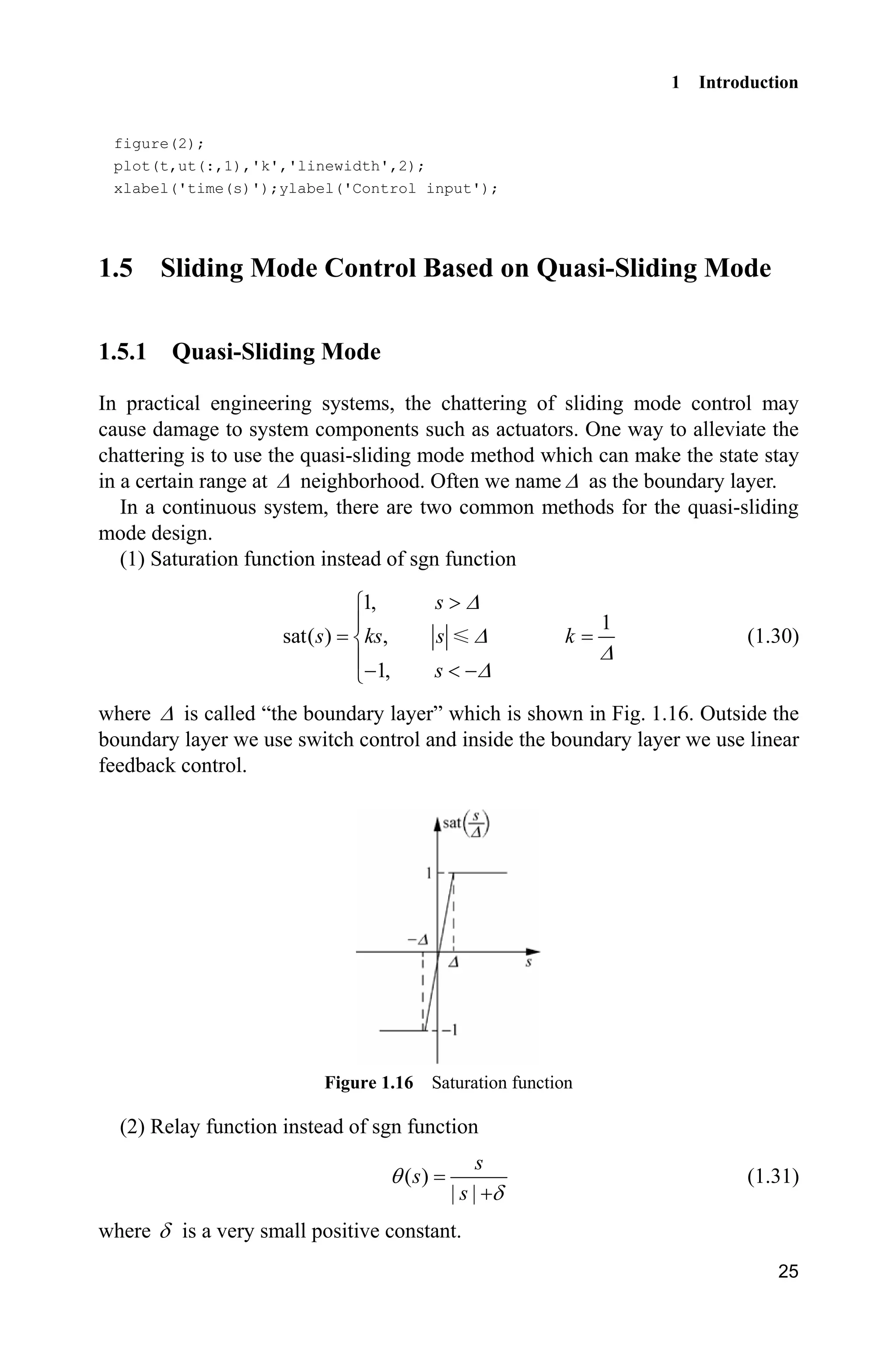
In order to restrain the chattering phenomenon, the saturated function sat( )s
is adopted instead of sgn( )s in Eq. (1.29) as
1,
sat( ) , | | , 1/
1,
s
s ks s k
s
'
' '
'
!
°
®
° ¯
(1.29)
where ' is the “boundary layer”.
The nature of saturated function is: out of the boundary layer, switch control is
selected, in the boundary layer, the usual feedback control is adopted. Therefore,
the chattering phenomenon can be restrained thoroughly.
1.4.3 Simulation Example
The dynamic equation of inverted pendulum is
1 2
2 ( ) ( )
x x
x f g u
®
˜¯ x x
where
2
1 2 1 1 c
2
1 c
sin cos sin /( )
( )
(4/3 cos /( ))
g x mlx x x m m
f
l m x m m
x
1 c
2
1 c
cos /( )
( )
(4/3 cos /( ))
x m m
g
l m x m m
x
where 1 2[ ],x xx 1x and 2x are the oscillation angle and oscillation rate respec-
tively, 2
9.8 m/s ,g cm is the vehicle mass, c 1kg,m m is the mass of pendulum
bar, 0.1kg,m l is one half of pendulum length, 0.5 m,l u is the control input.
Figure 1.11 Inverted pendulum system
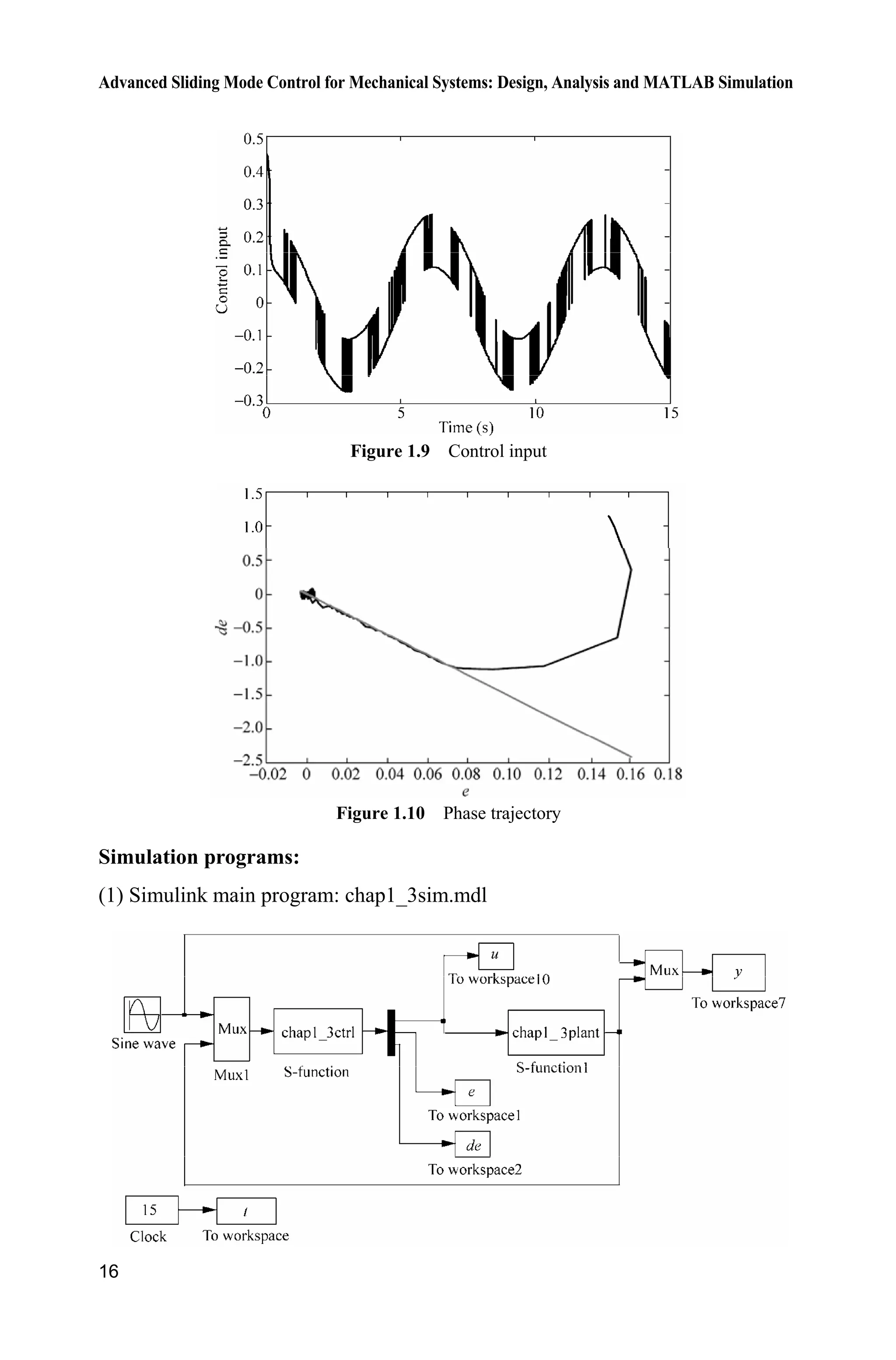
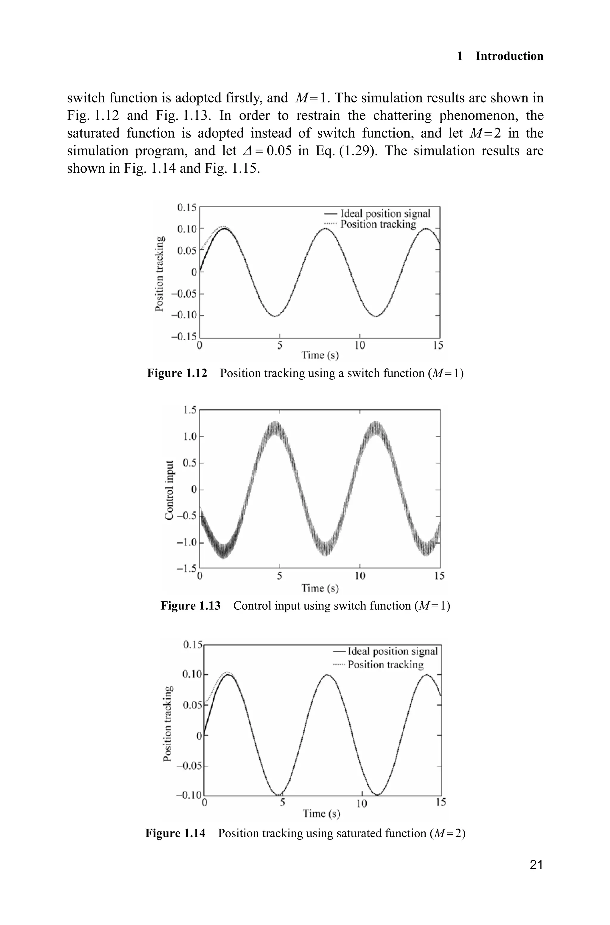
Let 1 ,x T and the desired trajectory is d ( ) 0.1sin ( ).t tT The initial state of
the inverted pendulum is [ / 60 0],S and 0.20.K The controller is Eq. (1.28)
M is a variable in the simulation program. M 1 indicates the controller with a
switch function, and M 2 indicates the controller with a saturation function. The](https://image.slidesharecdn.com/advancedslidingmodecontrolformechanicalsystems-130611121131-phpapp01/75/Advanced-sliding-mode-control-for-mechanical-systems-34-2048.jpg)
![Advanced Sliding Mode Control for Mechanical Systems: Design, Analysis and MATLAB Simulation
22
Figure 1.15 Control input using saturated function (M 2)
Simulation programs:
(1) Simulink main program: chap1_4sim.mdl
(2) S-function of controller: chap1_4ctrl.m
function [sys,x0,str,ts] = spacemodel(t,x,u,flag)
switch flag,
case 0,
[sys,x0,str,ts]=mdlInitializeSizes;
case 3,
sys=mdlOutputs(t,x,u);
case {1,2,4,9}
sys=[];
otherwise
error(['Unhandled flag = ',num2str(flag)]);
end
function [sys,x0,str,ts]=mdlInitializeSizes
sizes = simsizes;
sizes.NumContStates = 0;
sizes.NumDiscStates = 0;](https://image.slidesharecdn.com/advancedslidingmodecontrolformechanicalsystems-130611121131-phpapp01/75/Advanced-sliding-mode-control-for-mechanical-systems-36-2048.jpg)
![1 Introduction
23
sizes.NumOutputs = 1;
sizes.NumInputs = 3;
sizes.DirFeedthrough = 1;
sizes.NumSampleTimes = 0;
sys = simsizes(sizes);
x0 = [];
str = [];
ts = [];
function sys=mdlOutputs(t,x,u)
r=0.1*sin(t);
dr=0.1*cos(t);
ddr=-0.1*sin(t);
x1=u(2);
x2=u(3);
e=r-x1;
de=dr-x2;
c=1.5;
s=c*e+de;
g=9.8;mc=1.0;m=0.1;l=0.5;
T=l*(4/3-m*(cos(x1))^2/(mc+m));
fx=g*sin(x1)-m*l*x2^2*cos(x1)*sin(x1)/(mc+m);
fx=fx/T;
gx=cos(x1)/(mc+m);
gx=gx/T;
xite=0.20;
M=2;
if M==1
ut=1/gx*(-fx+ddr+c*de+xite*sign(s));
elseif M==2 %Saturated function
delta=0.05;
kk=1/delta;
if abs(s)delta
sats=sign(s);
else
sats=kk*s;
end
ut=1/gx*(-fx+ddr+c*de+xite*sats);
end
sys(1)=ut;
(3) S-function of the plant: chap1_4plant.m
function [sys,x0,str,ts]=s_function(t,x,u,flag)](https://image.slidesharecdn.com/advancedslidingmodecontrolformechanicalsystems-130611121131-phpapp01/75/Advanced-sliding-mode-control-for-mechanical-systems-37-2048.jpg)
![Advanced Sliding Mode Control for Mechanical Systems: Design, Analysis and MATLAB Simulation
24
switch flag,
case 0,
[sys,x0,str,ts]=mdlInitializeSizes;
case 1,
sys=mdlDerivatives(t,x,u);
case 3,
sys=mdlOutputs(t,x,u);
case {2, 4, 9 }
sys = [];
otherwise
error(['Unhandled flag = ',num2str(flag)]);
end
function [sys,x0,str,ts]=mdlInitializeSizes
sizes = simsizes;
sizes.NumContStates = 2;
sizes.NumDiscStates = 0;
sizes.NumOutputs = 2;
sizes.NumInputs = 1;
sizes.DirFeedthrough = 0;
sizes.NumSampleTimes = 0;
sys=simsizes(sizes);
x0=[pi/60 0];
str=[];
ts=[];
function sys=mdlDerivatives(t,x,u)
g=9.8;mc=1.0;m=0.1;l=0.5;
S=l*(4/3-m*(cos(x(1)))^2/(mc+m));
fx=g*sin(x(1))-m*l*x(2)^2*cos(x(1))*sin(x(1))/(mc+m);
fx=fx/S;
gx=cos(x(1))/(mc+m);
gx=gx/S;
%%%%%%%%%
dt=0*10*sin(t);
%%%%%%%%%
sys(1)=x(2);
sys(2)=fx+gx*u+dt;
function sys=mdlOutputs(t,x,u)
sys(1)=x(1);
sys(2)=x(2);
(4) plot program: chap1_4plot.m
close all;
figure(1);
plot(t,y(:,1),'k',t,y(:,2),'r:','linewidth',2);
legend('Ideal position signal','Position tracking');
xlabel('time(s)');ylabel('Position tracking');](https://image.slidesharecdn.com/advancedslidingmodecontrolformechanicalsystems-130611121131-phpapp01/75/Advanced-sliding-mode-control-for-mechanical-systems-38-2048.jpg)
![1 Introduction
29
(2) Controller: chap1_5ctrl.m
function [sys,x0,str,ts] = spacemodel(t,x,u,flag)
switch flag,
case 0,
[sys,x0,str,ts]=mdlInitializeSizes;
case 3,
sys=mdlOutputs(t,x,u);
case {2,4,9}
sys=[];
otherwise
error(['Unhandled flag = ',num2str(flag)]);
end
function [sys,x0,str,ts]=mdlInitializeSizes
sizes = simsizes;
sizes.NumContStates = 0;
sizes.NumDiscStates = 0;
sizes.NumOutputs = 3;
sizes.NumInputs = 3;
sizes.DirFeedthrough = 1;
sizes.NumSampleTimes = 0;
sys = simsizes(sizes);
x0 = [];
str = [];
ts = [];
function sys=mdlOutputs(t,x,u)
r=u(1);
dr=cos(t);
ddr=-sin(t);
th=u(2);
dth=u(3);
c=15;
e=r-th;
de=dr-dth;
s=c*e+de;
D=50;
xite=1.50;
fx=25*dth;
b=133;
M=2;
if M==1 %Switch function
ut=1/b*(c*(dr-dth)+ddr+fx+(D+xite)*sign(s));
elseif M==2 %Saturated function
fai=0.20;
if abs(s)=fai](https://image.slidesharecdn.com/advancedslidingmodecontrolformechanicalsystems-130611121131-phpapp01/75/Advanced-sliding-mode-control-for-mechanical-systems-43-2048.jpg)
![Advanced Sliding Mode Control for Mechanical Systems: Design, Analysis and MATLAB Simulation
30
sat=s/fai;
else
sat=sign(s);
end
ut=1/b*(c*(dr-dth)+ddr+fx+(D+xite)*sat);
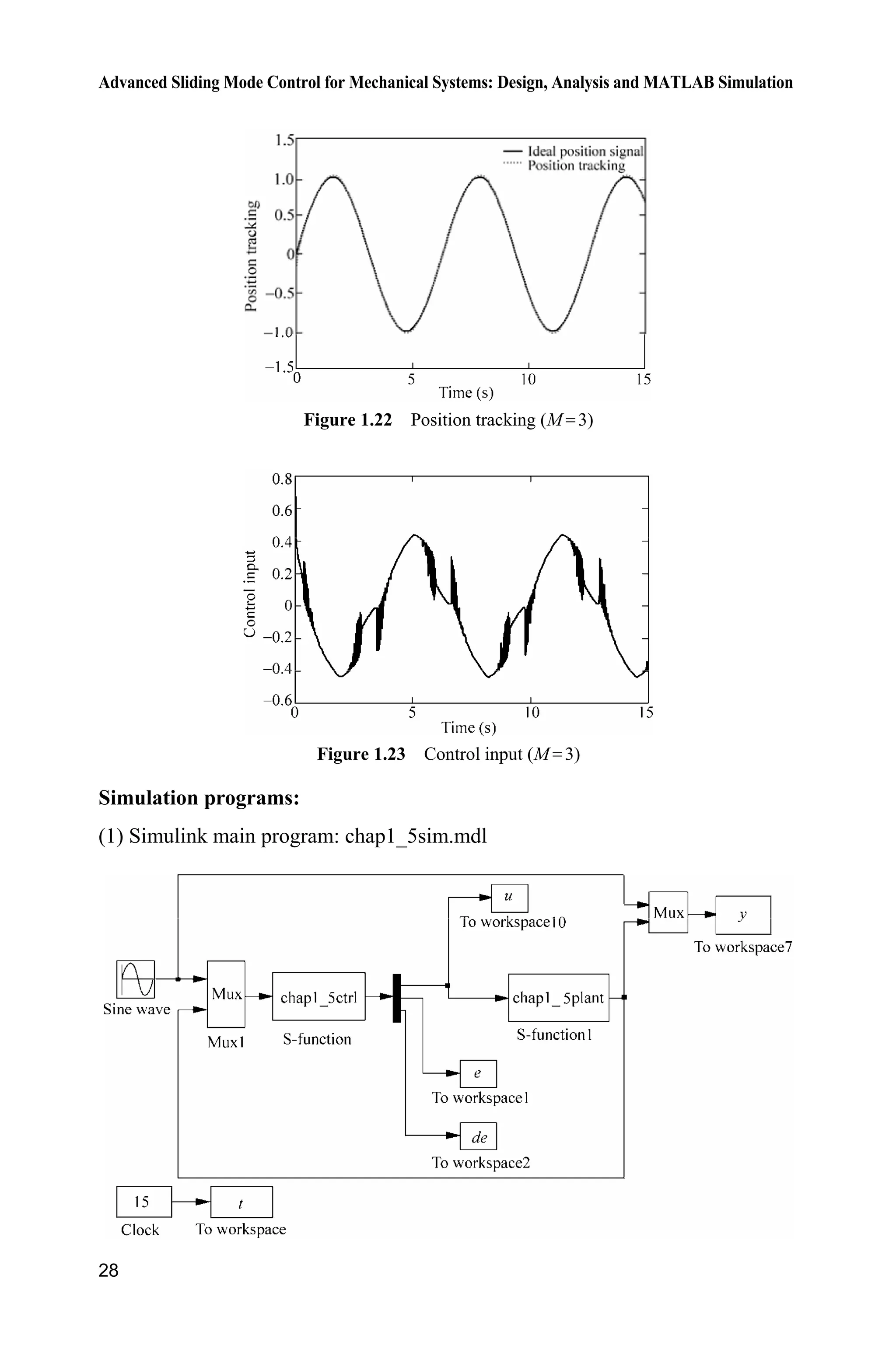
elseif M==3 %Relay function
delta=0.015;
rs=s/(abs(s)+delta);
ut=1/b*(c*(dr-dth)+ddr+fx+(D+xite)*rs);
end
sys(1)=ut;
sys(2)=e;
sys(3)=de;
(3) Plant: chap1_5plant.m
function [sys,x0,str,ts]=s_function(t,x,u,flag)
switch flag,
case 0,
[sys,x0,str,ts]=mdlInitializeSizes;
case 1,
sys=mdlDerivatives(t,x,u);
case 3,
sys=mdlOutputs(t,x,u);
case {2, 4, 9 }
sys = [];
otherwise
error(['Unhandled flag = ',num2str(flag)]);
end
function [sys,x0,str,ts]=mdlInitializeSizes
sizes = simsizes;
sizes.NumContStates = 2;
sizes.NumDiscStates = 0;
sizes.NumOutputs = 2;
sizes.NumInputs = 1;
sizes.DirFeedthrough = 0;
sizes.NumSampleTimes = 0;
sys=simsizes(sizes);
x0=[-0.15 -0.15];
str=[];
ts=[];
function sys=mdlDerivatives(t,x,u)
dt=50*sin(t);
sys(1)=x(2);
sys(2)=-25*x(2)+133*u+dt;
function sys=mdlOutputs(t,x,u)
sys(1)=x(1);
sys(2)=x(2);](https://image.slidesharecdn.com/advancedslidingmodecontrolformechanicalsystems-130611121131-phpapp01/75/Advanced-sliding-mode-control-for-mechanical-systems-44-2048.jpg)
![1 Introduction
31
(4) Plot program: chap1_5plot.m
close all;
figure(1);
plot(t,y(:,1),'k',t,y(:,2),'r:','linewidth',2);
legend('Ideal position signal','Position tracking');
xlabel('time(s)');ylabel('Position tracking');
figure(2);
plot(t,u(:,1),'k','linewidth',2);
xlabel('time(s)');ylabel('Control input');
c=15;
figure(3);
plot(e,de,'k',e,-c'.*e,'r','linewidth',2);
xlabel('e');ylabel('de');
1.6 Sliding Mode Control Based on the Equivalent Control
In the sliding mode controller, the control law usually consists of the equivalent
control equ and the switching control sw .u The equivalent control keeps the state
of system on the sliding surface, while the switching control forces the system
sliding on the sliding surface.
1.6.1 System Description
A n -order SISO nonlinear system can be described as
( )
( , ) ( ) ( )n
x f x t bu t d t (1.32)
( 1) T
[ ]n
x x x
x (1.33)
where 0b ! , ,n
xR ,u R ( )d t denotes external disturbance and uncertainty
while we assume | ( ) | .d t D
1.6.2 Sliding Mode Controller Design
1.6.2.1 Equivalent Controller Design
Ignoring external disturbance and uncertainty, the plant can be described as](https://image.slidesharecdn.com/advancedslidingmodecontrolformechanicalsystems-130611121131-phpapp01/75/Advanced-sliding-mode-control-for-mechanical-systems-45-2048.jpg)
![Advanced Sliding Mode Control for Mechanical Systems: Design, Analysis and MATLAB Simulation
32
( )
( , ) ( )n
x f x t bu t (1.34)
The tracking error vector is
( 1) T
d [ ]n
e e e
e x x (1.35)
Then switch function is
( 1)
1 2( , ) n
s x t c e c e e
Ce (1.36)
where 1 2 1[ 1]nc c c C is a 1un vector.
Choose 0s , we get
( ) ( 1) ( ) ( )
1 2 1 2 1 d
1
( ) ( )
d
1
( , )
( , ) ( ) 0
n n n n
n
n
i n
i
i
s x t c e c e e c e c e c e x x
c e x f x t bu t
¦
(1.37)
The control law is designed as
1
( ) ( )
eq d
1
1
( , )
n
i n
i
i
u c e x f x t
b
§ ·
¨ ¸
© ¹
¦ (1.38)
1.6.2.2 Sliding Mode Controller Design
In order to satisfy reaching conditions of sliding mode control ( , ) ( , )s x t s x t˜
| |,sK 0K ! , we must choose switching control whose control law is
sw
1
sgn( )u K s
b
(1.39)
where .K D K
The sliding mode controller include the equivalent control and the switching
control, then we have
eq swu u u (1.40)
Stability proof:
1
( ) ( )
d
1
( , ) ( , ) ( ) ( )
n
i n
i
i
s x t c e x f x t bu t d t
¦ (1.41)
Submitting Eqs. (1.40) (1.41), we can get:
1 1
( ) ( ) ( ) ( )
d d
1 1
1 1
( , ) ( , ) ( , ) sgn( ) ( )
sgn( ) ( )
n n
i n i n
i i
i i
s x t c e x f x t b c e x f x t K s d t
b b
K s d t
§ ·§ ·
¨ ¸¨ ¸
© ¹© ¹
¦ ¦](https://image.slidesharecdn.com/advancedslidingmodecontrolformechanicalsystems-130611121131-phpapp01/75/Advanced-sliding-mode-control-for-mechanical-systems-46-2048.jpg)
![Advanced Sliding Mode Control for Mechanical Systems: Design, Analysis and MATLAB Simulation
34
Simulation programs:
(1) Simulink main program: chap1_6sim.mdl
(2) Controller: chap1_6ctrl.m
function [sys,x0,str,ts]=s_function(t,x,u,flag)
switch flag,
case 0,
[sys,x0,str,ts]=mdlInitializeSizes;
case 3,
sys=mdlOutputs(t,x,u);
case {2, 4, 9 }
sys = [];
otherwise
error(['Unhandled flag = ',num2str(flag)]);
end
function [sys,x0,str,ts]=mdlInitializeSizes
sizes = simsizes;
sizes.NumContStates = 0;
sizes.NumDiscStates = 0;
sizes.NumOutputs = 1;
sizes.NumInputs = 3;
sizes.DirFeedthrough = 1;
sizes.NumSampleTimes = 0;
sys=simsizes(sizes);
x0=[];
str=[];
ts=[];
function sys=mdlOutputs(t,x,u)
r=u(1);
dr=2*pi*cos(2*pi*t);
ddr=-(2*pi)^2*sin(2*pi*t);
x=u(2);dx=u(3);
e=r-x;
de=dr-dx;](https://image.slidesharecdn.com/advancedslidingmodecontrolformechanicalsystems-130611121131-phpapp01/75/Advanced-sliding-mode-control-for-mechanical-systems-48-2048.jpg)
![1 Introduction
35
c=25;
s=c*e+de;
f=-25*dx;
b=133;
ueq=1/b*(c*de+ddr-f);
D=50;
xite=0.10;
K=D+xite;
usw=1/b*K*sign(s);
ut=ueq+usw;
sys(1)=ut;
(3) Plant: chap1_6plant.m
function [sys,x0,str,ts]=s_function(t,x,u,flag)
switch flag,
case 0,
[sys,x0,str,ts]=mdlInitializeSizes;
case 1,
sys=mdlDerivatives(t,x,u);
case 3,
sys=mdlOutputs(t,x,u);
case {2, 4, 9 }
sys = [];
otherwise
error(['Unhandled flag = ',num2str(flag)]);
end
function [sys,x0,str,ts]=mdlInitializeSizes
sizes = simsizes;
sizes.NumContStates = 2;
sizes.NumDiscStates = 0;
sizes.NumOutputs = 2;
sizes.NumInputs = 1;
sizes.DirFeedthrough = 0;
sizes.NumSampleTimes = 0;
sys=simsizes(sizes);
x0=[0,0];
str=[];
ts=[];
function sys=mdlDerivatives(t,x,u)
dt=50*sin(t);
sys(1)=x(2);
sys(2)=-25*x(2)+133*u+dt;
function sys=mdlOutputs(t,x,u)
sys(1)=x(1);
sys(2)=x(2);](https://image.slidesharecdn.com/advancedslidingmodecontrolformechanicalsystems-130611121131-phpapp01/75/Advanced-sliding-mode-control-for-mechanical-systems-49-2048.jpg)
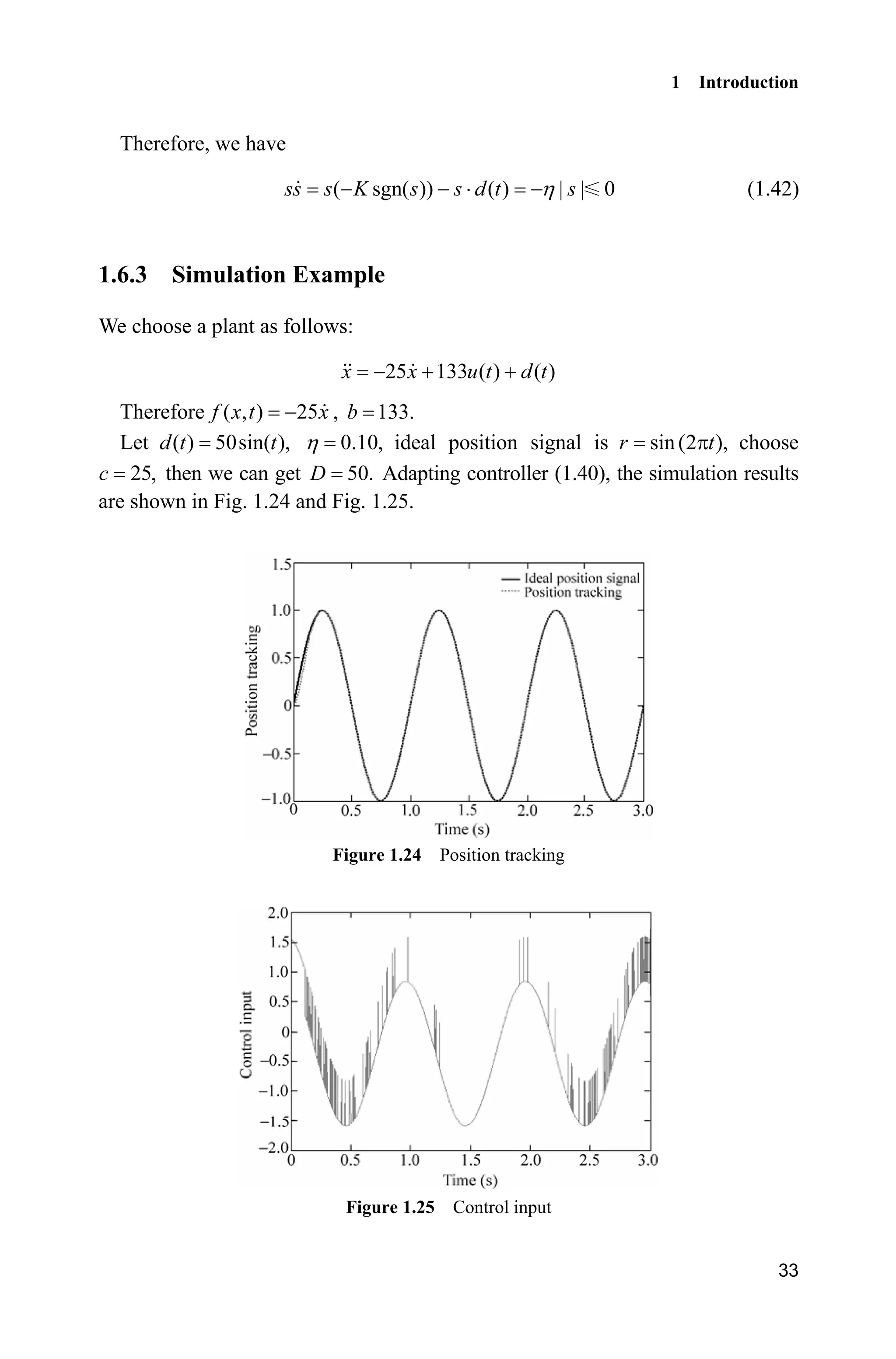
![1 Introduction
39
Figure 1.33 Control input
Simulation programs:
(1) Main program: chap1_7.m
clear all;
close all;
a=25;b=133;
xk=zeros(2,1);
ut_1=0;
c=5;
T=0.001;
for k=1:1:6000
time(k)=k*T;
thd(k)=sin(k*T);
dthd(k)=cos(k*T);
ddthd(k)=-sin(k*T);
tSpan=[0 T];
para=ut_1; % D/A
[tt,xx]=ode45('chap1_7plant',tSpan,xk,[],para);
xk=xx(length(xx),:); % A/D
th(k)=xk(1);
dth(k)=xk(2);
e(k)=thd(k)-th(k);
de(k)=dthd(k)-dth(k);
s(k)=c*e(k)+de(k);
xite=3.1; % xitemax(dt)
M=1;
if M==1
ut(k)=1/b*(a*dth(k)+ddthd(k)+c*de(k)+xite*sign(s(k)));
elseif M==2 %Saturated function
delta=0.05;
kk=1/delta;](https://image.slidesharecdn.com/advancedslidingmodecontrolformechanicalsystems-130611121131-phpapp01/75/Advanced-sliding-mode-control-for-mechanical-systems-53-2048.jpg)
![Advanced Sliding Mode Control for Mechanical Systems: Design, Analysis and MATLAB Simulation
40
if abs(s(k))delta
sats=sign(s(k));
else
sats=kk*s(k);
end
ut(k)=1/b*(a*dth(k)+ddthd(k)+c*de(k)+xite*sats);
end
ut_1=ut(k);
end
figure(1);
subplot(211);
plot(time,thd,'k',time,th,'r:','linewidth',2);
xlabel('time(s)');ylabel('position tracking');
legend('ideal position signal','tracking position signal');
subplot(212);
plot(time,dthd,'k',time,dth,'r:','linewidth',2);
xlabel('time(s)');ylabel('speed tracking');
legend('ideal speed signal','tracking speed signal');
figure(2);
plot(thd-th,dthd-dth,'k:',thd-th,-c*(thd-th),'r','linewidth',2);
%Draw line(s=0)
xlabel('e');ylabel('de');
legend('ideal sliding mode','phase trajectory');
figure(3);
plot(time,ut,'r','linewidth',2);
xlabel('time(s)');ylabel('Control input');
(2) Plant program: chap1_7plant.m
function dx=Plant(t,x,flag,para)
dx=zeros(2,1);
a=25;b=133;
ut=para(1);
dt=3.0*sin(t);
dx(1)=x(2);
dx(2)=-a*x(2)+b*ut+dt;
References
[1] Itkis U. Control System of Variable Structure. New York: Wiley, 1976
[2] Hung JY, Gao W, Hung JC. Variable Structure Control: A Survey, IEEE Transaction on
Industrial Electronics, 1993,40(1): 2 22
[3] Edwards C, Spurgeon S. Sliding Mode Control: Theory and Applications, London: Taylor
and Francis, 1998](https://image.slidesharecdn.com/advancedslidingmodecontrolformechanicalsystems-130611121131-phpapp01/75/Advanced-sliding-mode-control-for-mechanical-systems-54-2048.jpg)
![2 Normal Sliding Mode Control
45
From 21
,
2
V Js we get 2
,Jss Ks i.e. 2
.
K
ss s
J
Therefore, we have
( ) (0) exp
K
s t s t
J
§ ·
¨ ¸
© ¹
Finally, we can find that ( )s t is exponentially convergent.
2.1.5 Simulation
Consider the system as follows:
J B u dT T
where 10 3sin (2 )B t S , 3 0.5sin (2 )J t S , and ( ) 10sind t t .
Let n 10,B n 3,J and we get m 7,B M 13,B m 2.5,J M 3.5,J M 10.d
We select 1.0,k therefore, n
2
n
2 ,
B
h k
J
2
1 .h k In Eq. (2.11), select O n
n
B
J
10
,
3
10,K and the desired trajectory is d ( ) sin ,t tT the initial state vector is
[0.5 0]. The simulation results are shown in Fig. 2.2 Fig. 2.4.
Figure 2.2 Position tracking
Figure 2.3 Velocity tracking](https://image.slidesharecdn.com/advancedslidingmodecontrolformechanicalsystems-130611121131-phpapp01/75/Advanced-sliding-mode-control-for-mechanical-systems-59-2048.jpg)
![Advanced Sliding Mode Control for Mechanical Systems: Design, Analysis and MATLAB Simulation
46
Figure 2.4 Control input
Simulation programs:
(1) Simulink main program: chap2_1sim.mdl
(2) S-function of controller for the nominal model: chap2_1ctrl1.m
function [sys,x0,str,ts]=s_function(t,x,u,flag)
switch flag,
case 0,
[sys,x0,str,ts]=mdlInitializeSizes;
case 3,
sys=mdlOutputs(t,x,u);
case {2, 4, 9 }
sys = [];
otherwise
error(['Unhandled flag = ',num2str(flag)]);
end
function [sys,x0,str,ts]=mdlInitializeSizes
sizes = simsizes;
sizes.NumContStates = 0;
sizes.NumDiscStates = 0;](https://image.slidesharecdn.com/advancedslidingmodecontrolformechanicalsystems-130611121131-phpapp01/75/Advanced-sliding-mode-control-for-mechanical-systems-60-2048.jpg)
![2 Normal Sliding Mode Control
47
sizes.NumOutputs = 1;
sizes.NumInputs = 3;
sizes.DirFeedthrough = 1;
sizes.NumSampleTimes = 0;
sys=simsizes(sizes);
x0=[];
str=[];
ts=[];
function sys=mdlOutputs(t,x,u)
thn=u(1);
dthn=u(2);
thd=u(3);dthd=cos(t);ddthd=-sin(t);
e=thn-thd;
de=dthn-dthd;
k=3;
Bn=10;Jn=3;
h1=k^2;
h2=2*k-Bn/Jn;
ut=Jn*(-h1*e-h2*de+Bn/Jn*dthd+ddthd);
sys(1)=ut;
(3) S-function of nominal model: chap2_1model.m
function [sys,x0,str,ts]=s_function(t,x,u,flag)
switch flag,
case 0,
[sys,x0,str,ts]=mdlInitializeSizes;
case 1,
sys=mdlDerivatives(t,x,u);
case 3,
sys=mdlOutputs(t,x,u);
case {2, 4, 9 }
sys = [];
otherwise
error(['Unhandled flag = ',num2str(flag)]);
end
function [sys,x0,str,ts]=mdlInitializeSizes
sizes = simsizes;
sizes.NumContStates = 2;
sizes.NumDiscStates = 0;
sizes.NumOutputs = 2;
sizes.NumInputs = 1;
sizes.DirFeedthrough = 0;
sizes.NumSampleTimes = 0;
sys=simsizes(sizes);
x0=[0.5,0];
str=[];
ts=[];
function sys=mdlDerivatives(t,x,u)](https://image.slidesharecdn.com/advancedslidingmodecontrolformechanicalsystems-130611121131-phpapp01/75/Advanced-sliding-mode-control-for-mechanical-systems-61-2048.jpg)
![Advanced Sliding Mode Control for Mechanical Systems: Design, Analysis and MATLAB Simulation
48
Bn=10;
Jn=3;
sys(1)=x(2);
sys(2)=1/Jn*(u-Bn*x(2));
function sys=mdlOutputs(t,x,u)
sys(1)=x(1);
sys(2)=x(2);
(4) S-function of sliding mode controller for the actual plant: chap2_1ctrl2.m
function [sys,x0,str,ts]=s_function(t,x,u,flag)
switch flag,
case 0,
[sys,x0,str,ts]=mdlInitializeSizes;
case 3,
sys=mdlOutputs(t,x,u);
case {2, 4, 9 }
sys = [];
otherwise
error(['Unhandled flag = ',num2str(flag)]);
end
function [sys,x0,str,ts]=mdlInitializeSizes
sizes = simsizes;
sizes.NumContStates = 0;
sizes.NumDiscStates = 0;
sizes.NumOutputs = 1;
sizes.NumInputs = 5;
sizes.DirFeedthrough = 1;
sizes.NumSampleTimes = 0;
sys=simsizes(sizes);
x0=[];
str=[];
ts=[];
function sys=mdlOutputs(t,x,u)
Bn=10;Jn=3;
lamt=Bn/Jn;
Jm=2.5;JM=3.5;
Bm=7;BM=13;
dM=0.10;
K=10;
thn=u(1);dthn=u(2);
nu=u(3);
th=u(4);dth=u(5);
en=th-thn;
den=dth-dthn;
s=den+lamt*en;
temp0=(1/Jn)*nu-lamt*dth;](https://image.slidesharecdn.com/advancedslidingmodecontrolformechanicalsystems-130611121131-phpapp01/75/Advanced-sliding-mode-control-for-mechanical-systems-62-2048.jpg)
![2 Normal Sliding Mode Control
49
Ja=1/2*(JM+Jm);
Ba=1/2*(BM+Bm);
h=dM+1/2*(JM-Jm)*abs(temp0)+1/2*(BM-Bm)*abs(dth);
ut=-K*s-h*sign(s)+Ja*((1/Jn)*nu-lamt*dth)+Ba*dth;
sys(1)=ut;
(5) S-function of the actual plant: chap2_1plant.m
function [sys,x0,str,ts]=s_function(t,x,u,flag)
switch flag,
case 0,
[sys,x0,str,ts]=mdlInitializeSizes;
case 1,
sys=mdlDerivatives(t,x,u);
case 3,
sys=mdlOutputs(t,x,u);
case {2, 4, 9 }
sys = [];
otherwise
error(['Unhandled flag = ',num2str(flag)]);
end
function [sys,x0,str,ts]=mdlInitializeSizes
sizes = simsizes;
sizes.NumContStates = 2;
sizes.NumDiscStates = 0;
sizes.NumOutputs = 2;
sizes.NumInputs = 1;
sizes.DirFeedthrough = 0;
sizes.NumSampleTimes = 0;
sys=simsizes(sizes);
x0=[0.5,0];
str=[];
ts=[];
function sys=mdlDerivatives(t,x,u)
d=0.10*sin(t);
B=10+3*sin(2*pi*t);
J=3+0.5*sin(2*pi*t);
sys(1)=x(2);
sys(2)=1/J*(u-B*x(2)-d);
function sys=mdlOutputs(t,x,u)
sys(1)=x(1);
sys(2)=x(2);
(6) Plot program: chap2_1plot.m
close all;
figure(1);
plot(t,sin(t),'k',t,y(:,2),'r:','linewidth',2);](https://image.slidesharecdn.com/advancedslidingmodecontrolformechanicalsystems-130611121131-phpapp01/75/Advanced-sliding-mode-control-for-mechanical-systems-63-2048.jpg)
![2 Normal Sliding Mode Control
51
2.2.2 Global Sliding Mode Design
Let the desired trajectory be dT and the tracking error be:
de T T (2.16)
The global dynamic sliding mode variable is designed as
( )s e ce f t (2.17)
where 0,c ! ( )f t is a function to be designed so as to attain at the sliding
surface, and ( )f t is satisfied with the following conditions[1]
: (1) (0)f
0 0 ;e ce (2) ( ) 0f t o as ;t o f and (3) ( )f t is derivable.
From the above three conditions, ( )f t can be designed as
( ) (0)e kt
f t f
(2.18)
2.2.3 Sliding Mode Controller Design
The global sliding mode controller is designed as
d d d d
ˆ ˆ( ) ( ) ( | | | |)sgn( )u J c f J c J c f D J c sT T T T T T ' ' (2.19)
where,
max minˆ ,
2
J J
J
max min
2
J J
J
' (2.20)
Let the Lyapunov function be
21
2
V s (2.21)
From Eq. (2.17), we have
d d
d d
1 1
d d
( )
( ) ( )
( ( ) ( ) )
s e ce f c f
bu bd c f c
b b c f b c u d
T T T T
T T T
T T T
and from Eq. (2.19), we have
1 1 1
d d d d
d d
1 1
d d
d d
ˆ ˆ( ) ( ) ( ) ( )
| | | |)sgn( )
ˆ ˆ( )( ) | | sgn( ) ( )( )
| | sgn( ) sgn( )
b s b c f b c J c f J c
J c f D J c s d
b J c f J c f s b J c
J c s d D s
T T T T T T
T T T
T T T T
T T
' '
'
'](https://image.slidesharecdn.com/advancedslidingmodecontrolformechanicalsystems-130611121131-phpapp01/75/Advanced-sliding-mode-control-for-mechanical-systems-65-2048.jpg)
![Advanced Sliding Mode Control for Mechanical Systems: Design, Analysis and MATLAB Simulation
54
Simulation programs:
(1) Simulink main program: chap2_2sim.mdl
(2) S-function of controller: chap2_2ctrl.m
function [sys,x0,str,ts] = spacemodel(t,x,u,flag)
switch flag,
case 0,
[sys,x0,str,ts]=mdlInitializeSizes;
case 3,
sys=mdlOutputs(t,x,u);
case {2,4,9}
sys=[];
otherwise
error(['Unhandled flag = ',num2str(flag)]);
end
function [sys,x0,str,ts]=mdlInitializeSizes
sizes = simsizes;
sizes.NumContStates = 0;
sizes.NumDiscStates = 0;
sizes.NumOutputs = 2;
sizes.NumInputs = 3;
sizes.DirFeedthrough = 1;
sizes.NumSampleTimes = 1;
sys = simsizes(sizes);
x0 = [];
str = [];
ts = [0 0];
function sys=mdlOutputs(t,x,u)
thd=u(1);
dthd=cos(t);](https://image.slidesharecdn.com/advancedslidingmodecontrolformechanicalsystems-130611121131-phpapp01/75/Advanced-sliding-mode-control-for-mechanical-systems-68-2048.jpg)
![2 Normal Sliding Mode Control
55
ddthd=-sin(t);
th=u(2);
dth=u(3);
c=10;
e=th-thd;
de=dth-dthd;
dt=0.10*sin(2*pi*t);
D=0.10;
e0=pi/6;
de0=0-1.0;
s0=de0+c*e0;
ft=s0*exp(-130*t);
df=-130*s0*exp(-130*t);
s=de+c*e-ft;
R=ddthd+c*dthd;
J_min=0.80;
J_max=1.20;
aJ=(J_min+J_max)/2;
dJ=(J_max-J_min)/2;
M=2;
if M==1
ut=-aJ*(c*dth-df)+aJ*R-[dJ*abs(c*dth-df)+D+dJ*abs(R)]*sign(s);
elseif M==2
fai=0.05;
if s/fai1
sat=1;
elseif abs(s/fai)=1
sat=s/fai;
elseif s/fai-1
sat=-1;
end
ut=-aJ*(c*dth-df)+aJ*R-[dJ*abs(c*dth-df)+D+dJ*abs(R)]*sat;
end
sys(1)=ut;
sys(2)=s;
(3) S-function of the plant: chap2_2plant.m
function [sys,x0,str,ts] = spacemodel(t,x,u,flag)
switch flag,
case 0,
[sys,x0,str,ts]=mdlInitializeSizes;](https://image.slidesharecdn.com/advancedslidingmodecontrolformechanicalsystems-130611121131-phpapp01/75/Advanced-sliding-mode-control-for-mechanical-systems-69-2048.jpg)
![Advanced Sliding Mode Control for Mechanical Systems: Design, Analysis and MATLAB Simulation
56
case 1,
sys=mdlDerivatives(t,x,u);
case 3,
sys=mdlOutputs(t,x,u);
case {2,4,9}
sys=[];
otherwise
error(['Unhandled flag = ',num2str(flag)]);
end
function [sys,x0,str,ts]=mdlInitializeSizes
sizes = simsizes;
sizes.NumContStates = 2;
sizes.NumDiscStates = 0;
sizes.NumOutputs = 2;
sizes.NumInputs = 1;
sizes.DirFeedthrough = 0;
sizes.NumSampleTimes = 0;
sys = simsizes(sizes);
x0 = [pi/6;0];
str = [];
ts = [];
function sys=mdlDerivatives(t,x,u)
J=1.0+0.2*sin(t);
dt=0.10*sin(2*pi*t);
sys(1)=x(2);
sys(2)=1/J*(u-dt);
function sys=mdlOutputs(t,x,u)
sys(1)=x(1);
sys(2)=x(2);
(4) Plot program: chap2_2plot.m
close all;
figure(1);
figure(1);
plot(t,y(:,1),'k',t,y(:,2),'r:','linewidth',2);
xlabel('time(s)');ylabel('Position tracking');
legend('ideal position signal','tracking position signal');
figure(2);
plot(t,u(:,1),'r','linewidth',2);
xlabel('time(s)');ylabel('Control input');
figure(3);
plot(t,s(:,1),'r','linewidth',2);
xlabel('time(s)');ylabel('Switch function');](https://image.slidesharecdn.com/advancedslidingmodecontrolformechanicalsystems-130611121131-phpapp01/75/Advanced-sliding-mode-control-for-mechanical-systems-70-2048.jpg)
![Advanced Sliding Mode Control for Mechanical Systems: Design, Analysis and MATLAB Simulation
58
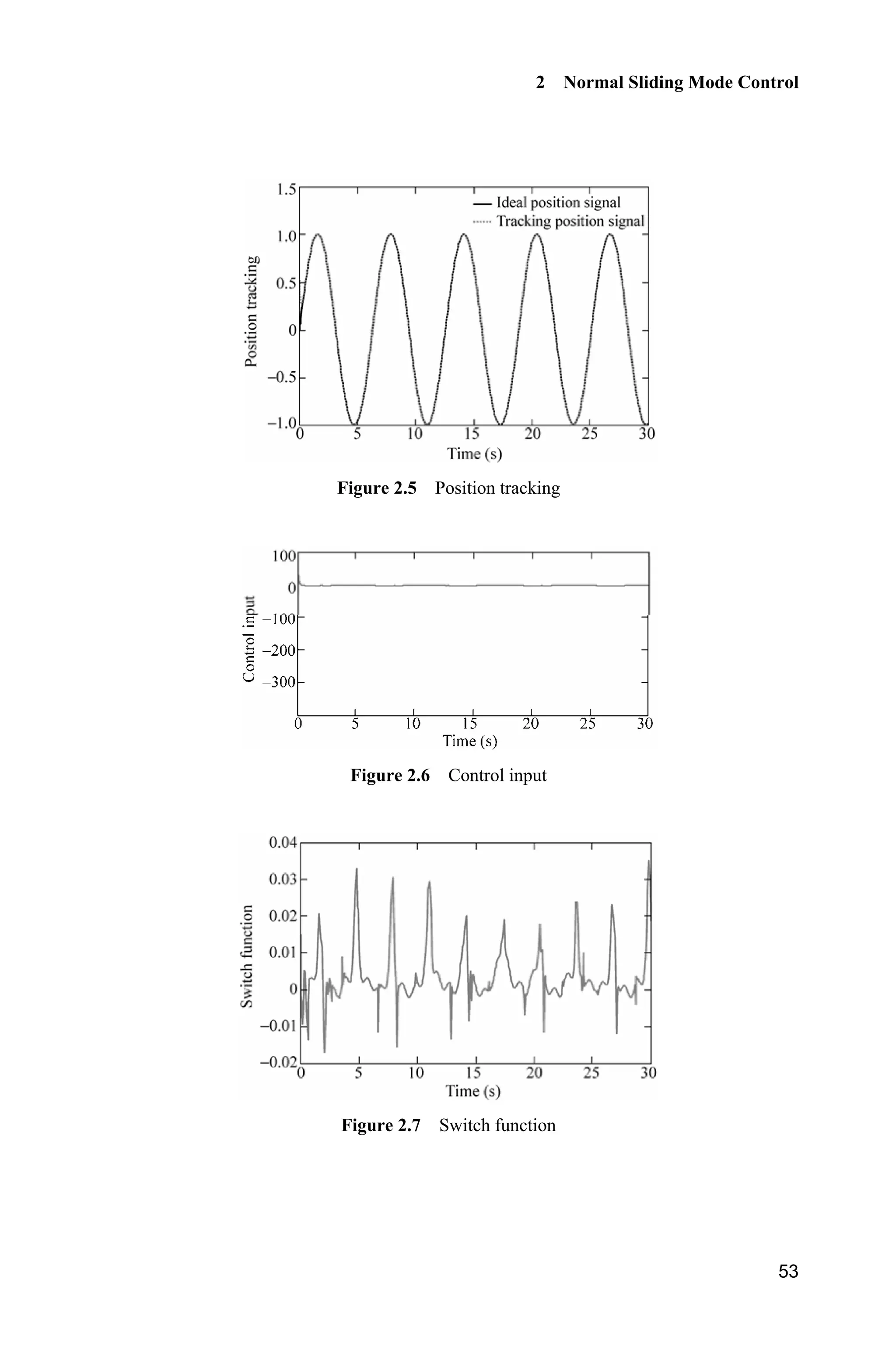
The desired trajectory is d ( ) 0.1sin ( ).x t tS Controller is Eq. (2.24), 1 2 5,k k
The initial state of the inverted pendulum is [ / 60 0].S The simulation results
are shown in Fig. 2.8 and Fig. 2.9.
Figure 2.8 Position tracking
Figure 2.9 Control input
Simulation programs:
(1) Simulink main program: chap2_3sim.mdl](https://image.slidesharecdn.com/advancedslidingmodecontrolformechanicalsystems-130611121131-phpapp01/75/Advanced-sliding-mode-control-for-mechanical-systems-72-2048.jpg)
![2 Normal Sliding Mode Control
59
(2) S-function of controller: chap2_3ctrl.m
function [sys,x0,str,ts] = spacemodel(t,x,u,flag)
switch flag,
case 0,
[sys,x0,str,ts]=mdlInitializeSizes;
case 1,
sys=mdlDerivatives(t,x,u);
case 3,
sys=mdlOutputs(t,x,u);
case {1,2,4,9}
sys=[];
otherwise
error(['Unhandled flag = ',num2str(flag)]);
end
function [sys,x0,str,ts]=mdlInitializeSizes
sizes = simsizes;
sizes.NumContStates = 0;
sizes.NumDiscStates = 0;
sizes.NumOutputs = 1;
sizes.NumInputs = 5;
sizes.DirFeedthrough = 1;
sizes.NumSampleTimes = 0;
sys = simsizes(sizes);
x0 = [];
str = [];
ts = [];
function sys=mdlOutputs(t,x,u)
r=0.1*sin(pi*t);
dr=0.1*pi*cos(pi*t);
ddr=-0.1*pi*pi*sin(pi*t);
e=u(1);
de=u(2);
fx=u(4);
gx=u(5);
k1=5;k2=5;
v=ddr+k1*e+k2*de;
ut=(v-fx)/(gx+0.002);
sys(1)=ut;
(3) S-function of the plant: chap2_3plant.m
function [sys,x0,str,ts]=s_function(t,x,u,flag)
switch flag,
case 0,
[sys,x0,str,ts]=mdlInitializeSizes;
case 1,](https://image.slidesharecdn.com/advancedslidingmodecontrolformechanicalsystems-130611121131-phpapp01/75/Advanced-sliding-mode-control-for-mechanical-systems-73-2048.jpg)
![Advanced Sliding Mode Control for Mechanical Systems: Design, Analysis and MATLAB Simulation
60
sys=mdlDerivatives(t,x,u);
case 3,
sys=mdlOutputs(t,x,u);
case {2, 4, 9 }
sys = [];
otherwise
error(['Unhandled flag = ',num2str(flag)]);
end
function [sys,x0,str,ts]=mdlInitializeSizes
sizes = simsizes;
sizes.NumContStates = 2;
sizes.NumDiscStates = 0;
sizes.NumOutputs = 3;
sizes.NumInputs = 1;
sizes.DirFeedthrough = 0;
sizes.NumSampleTimes = 0;
sys=simsizes(sizes);
x0=[pi/60 0];
str=[];
ts=[];
function sys=mdlDerivatives(t,x,u)
g=9.8;mc=1.0;m=0.1;l=0.5;
S=l*(4/3-m*(cos(x(1)))^2/(mc+m));
fx=g*sin(x(1))-m*l*x(2)^2*cos(x(1))*sin(x(1))/(mc+m);
fx=fx/S;
gx=cos(x(1))/(mc+m);
gx=gx/S;
sys(1)=x(2);
sys(2)=fx+gx*u;
function sys=mdlOutputs(t,x,u)
g=9.8;mc=1.0;m=0.1;l=0.5;
S=l*(4/3-m*(cos(x(1)))^2/(mc+m));
fx=g*sin(x(1))-m*l*x(2)^2*cos(x(1))*sin(x(1))/(mc+m);
fx=fx/S;
gx=cos(x(1))/(mc+m);
gx=gx/S;
sys(1)=x(1);
sys(2)=fx;
sys(3)=gx;
(4) Plot program: chap2_3plot.m
close all;
figure(1);
plot(t,y(:,1),'k',t,y(:,2),'r:','linewidth',2);
xlabel('time(s)');ylabel('Position tracking');
legend('Ideal position signal','tracking signal');](https://image.slidesharecdn.com/advancedslidingmodecontrolformechanicalsystems-130611121131-phpapp01/75/Advanced-sliding-mode-control-for-mechanical-systems-74-2048.jpg)
![2 Normal Sliding Mode Control
61
figure(2);
plot(t,ut(:,1),'k','linewidth',2);
xlabel('time(s)');ylabel('Control input');
2.3.3 Sliding Mode Control Based on Linearization Feedback
Consider the following second-order SISO uncertain nonlinear system:
( , ) ( , ) ( )x f x t g x t u d t (2.28)
where f and g are known nonlinear functions, ( )d t is the uncertainty, and
| ( ) | .d t D
Let the desired trajectory be d ,x therefore, we denote:
T
d [ ]e ee x x (2.29)
Sliding variable is selected as
( , )s x t ce (2.30)
where [ 1].cc
Based on linearization feedback technique, the sliding mode controller is
designed as
( , )
( , )
v f x t
u
g x t
(2.31)
d sgn( ),v x ce sK DK ! (2.32)
We select the Lyapunov function is
21
2
V s
therefore, we have
d
d
( ) ( )
( ( , ) ( , ) ( ) )
V ss s e ce s x x ce
s f x t g x t u d t x ce
From Eq. (2.31), we get
d
d d
( ( ) )
( sgn( ) ( ) )
( sgn( ) ( )) | | ( ) 0
V s v d t x ce
s x ce s d t x ce
s s d t s d t s
K
K K](https://image.slidesharecdn.com/advancedslidingmodecontrolformechanicalsystems-130611121131-phpapp01/75/Advanced-sliding-mode-control-for-mechanical-systems-75-2048.jpg)
![Advanced Sliding Mode Control for Mechanical Systems: Design, Analysis and MATLAB Simulation
62
2.3.4 Simulation Example
The dynamic equation of the inverted pendulum is
1 2
2
1 2 1 1 c 1 c
2 2 2
1 c 1 c
sin cos sin /( ) cos /( )
( )
(4/3 cos /( )) (4/3 cos /( ))
°
®
° ¯
x x
g x mlx x x m m x m m
x u d t
l m x m m l m x m m
where 1x and 2x are the oscillation angle and the oscillation rate respectively.
2
9.8 m/s ,g cm is the vehicle mass, c 1kg,m m is the mass of pendulum bar,
0.1kg,m l is one half of pendulum length, 0.5 m,l u is the control input.
( )d t is the disturbance.
The desired trajectory is d ( ) 0.1sin( ).x t tS The sliding variable is ,s ce e
where 10.c Controller is Eq. (2.31). The initial state of the inverted pendulum
is [ /60 0].S In the simulation program, M 1 denoes the sgn function is
adopted, and M 2 denotes the saturated function is adopted, and let M 2,
0 0.03,G 1 5,G 0 1 | |,G G G e 5.k The simulation results are shown in
Fig. 2.10 and Fig. 2.11.
Figure 2.10 Position tracking
Figure 2.11 Control input](https://image.slidesharecdn.com/advancedslidingmodecontrolformechanicalsystems-130611121131-phpapp01/75/Advanced-sliding-mode-control-for-mechanical-systems-76-2048.jpg)
![2 Normal Sliding Mode Control
63
Simulation programs:
(1) Simulink main program: chap2_4sim.mdl
(2) S-function of controller: chap2_4ctrl.m
function [sys,x0,str,ts] = spacemodel(t,x,u,flag)
switch flag,
case 0,
[sys,x0,str,ts]=mdlInitializeSizes;
case 1,
sys=mdlDerivatives(t,x,u);
case 3,
sys=mdlOutputs(t,x,u);
case {1,2,4,9}
sys=[];
otherwise
error(['Unhandled flag = ',num2str(flag)]);
end
function [sys,x0,str,ts]=mdlInitializeSizes
sizes = simsizes;
sizes.NumContStates = 0;
sizes.NumDiscStates = 0;
sizes.NumOutputs = 1;
sizes.NumInputs = 5;
sizes.DirFeedthrough = 1;
sizes.NumSampleTimes = 0;
sys = simsizes(sizes);
x0 = [];
str = [];
ts = [];
function sys=mdlOutputs(t,x,u)
r=0.1*sin(pi*t);
dr=0.1*pi*cos(pi*t);](https://image.slidesharecdn.com/advancedslidingmodecontrolformechanicalsystems-130611121131-phpapp01/75/Advanced-sliding-mode-control-for-mechanical-systems-77-2048.jpg)
![Advanced Sliding Mode Control for Mechanical Systems: Design, Analysis and MATLAB Simulation
64
ddr=-0.1*pi*pi*sin(pi*t);
e=u(1);
de=u(2);
fx=u(4);
gx=u(5);
c=10;
s=de+c*e;
M=1;
if M==1
xite=10;
v=ddr-c*de-xite*sign(s);
elseif M==2
xite=30;
delta0=0.03;
delta1=5;
delta=delta0+delta1*abs(e);
v=ddr-c*de-xite*s/(abs(s)+delta);
end
xx(1)=r+e;
xx(2)=dr+de;
ut=(-fx+v)/(gx+0.002);
sys(1)=ut;
(3) S-function of the plant: chap2_4plant.m
function [sys,x0,str,ts]=s_function(t,x,u,flag)
switch flag,
case 0,
[sys,x0,str,ts]=mdlInitializeSizes;
case 1,
sys=mdlDerivatives(t,x,u);
case 3,
sys=mdlOutputs(t,x,u);
case {2, 4, 9 }
sys = [];
otherwise
error(['Unhandled flag = ',num2str(flag)]);
end
function [sys,x0,str,ts]=mdlInitializeSizes
sizes = simsizes;
sizes.NumContStates = 2;
sizes.NumDiscStates = 0;
sizes.NumOutputs = 3;
sizes.NumInputs = 1;
sizes.DirFeedthrough = 0;](https://image.slidesharecdn.com/advancedslidingmodecontrolformechanicalsystems-130611121131-phpapp01/75/Advanced-sliding-mode-control-for-mechanical-systems-78-2048.jpg)
![2 Normal Sliding Mode Control
65
sizes.NumSampleTimes = 0;
sys=simsizes(sizes);
x0=[pi/60 0];
str=[];
ts=[];
function sys=mdlDerivatives(t,x,u)
g=9.8;mc=1.0;m=0.1;l=0.5;
S=l*(4/3-m*(cos(x(1)))^2/(mc+m));
fx=g*sin(x(1))-m*l*x(2)^2*cos(x(1))*sin(x(1))/(mc+m);
fx=fx/S;
gx=cos(x(1))/(mc+m);
gx=gx/S;
dt=10*sin(t);
sys(1)=x(2);
sys(2)=fx+gx*u+dt;
function sys=mdlOutputs(t,x,u)
g=9.8;mc=1.0;m=0.1;l=0.5;
S=l*(4/3-m*(cos(x(1)))^2/(mc+m));
fx=g*sin(x(1))-m*l*x(2)^2*cos(x(1))*sin(x(1))/(mc+m);
fx=fx/S;
gx=cos(x(1))/(mc+m);
gx=gx/S;
sys(1)=x(1);
sys(2)=fx;
sys(3)=gx;
(4) Plot program: chap2_4plot.m
close all;
figure(1);
plot(t,y(:,1),'k',t,y(:,2),'r:','linewidth',2);
xlabel('time(s)');ylabel('Position tracking');
legend('Ideal position signal','tracking signal');
figure(2);
plot(t,ut(:,1),'r','linewidth',2);
xlabel('time(s)');ylabel('Control input');
2.4 Input-Output Feedback Linearization Control
2.4.1 System Description
Consider the following system:](https://image.slidesharecdn.com/advancedslidingmodecontrolformechanicalsystems-130611121131-phpapp01/75/Advanced-sliding-mode-control-for-mechanical-systems-79-2048.jpg)
![Advanced Sliding Mode Control for Mechanical Systems: Design, Analysis and MATLAB Simulation
68
Simulation programs:
(1) Simulink main program: chap2_5sim.mdl
(2) Sub-program of controller: chap2_5ctrl.m
function [sys,x0,str,ts]=obser(t,x,u,flag)
switch flag,
case 0,
[sys,x0,str,ts]=mdlInitializeSizes;
case 1,
sys=mdlDerivatives(t,x,u);
case 3,
sys=mdlOutputs(t,x,u);
case {1, 2, 4, 9 }
sys = [];
otherwise
error(['Unhandled flag = ',num2str(flag)]);
end
function [sys,x0,str,ts]=mdlInitializeSizes
sizes = simsizes;
sizes.NumDiscStates = 0;
sizes.NumOutputs = 1;
sizes.NumInputs = 6;
sizes.DirFeedthrough = 1;
sizes.NumSampleTimes = 0;
sys=simsizes(sizes);
x0=[];
str=[];
ts=[];
function sys=mdlOutputs(t,x,u)
yd=u(1);
dyd=cos(t);
ddyd=-sin(t);](https://image.slidesharecdn.com/advancedslidingmodecontrolformechanicalsystems-130611121131-phpapp01/75/Advanced-sliding-mode-control-for-mechanical-systems-82-2048.jpg)
![2 Normal Sliding Mode Control
69
e=u(2);
de=u(3);
x1=u(4);
x2=u(5);
x3=u(6);
f=(x1^5+x3)*(x3+cos(x2))+(x2+1)*x1^2;
k1=10;k2=10;
v=ddyd+k1*e+k2*de;
ut=1.0/(x2+1)*(v-f);
sys(1)=ut;
(3) Sub-program of the plant: chap2_5plant.m
function [sys,x0,str,ts]=obser(t,x,u,flag)
switch flag,
case 0,
[sys,x0,str,ts]=mdlInitializeSizes;
case 1,
sys=mdlDerivatives(t,x,u);
case 3,
sys=mdlOutputs(t,x,u);
case {2, 4, 9 }
sys = [];
otherwise
error(['Unhandled flag = ',num2str(flag)]);
end
function [sys,x0,str,ts]=mdlInitializeSizes
sizes = simsizes;
sizes.NumContStates = 3;
sizes.NumDiscStates = 0;
sizes.NumOutputs = 3;
sizes.NumInputs = 1;
sizes.DirFeedthrough = 1;
sizes.NumSampleTimes = 0;
sys=simsizes(sizes);
x0=[0.15 0 0];
str=[];
ts=[];
function sys=mdlDerivatives(t,x,u)
ut=u(1);
sys(1)=sin(x(2))+(x(2)+1)*x(3);
sys(2)=x(1)^5+x(3);
sys(3)=x(1)^2+ut;
function sys=mdlOutputs(t,x,u)
sys(1)=x(1);
sys(2)=x(2);
sys(3)=x(3);](https://image.slidesharecdn.com/advancedslidingmodecontrolformechanicalsystems-130611121131-phpapp01/75/Advanced-sliding-mode-control-for-mechanical-systems-83-2048.jpg)
![2 Normal Sliding Mode Control
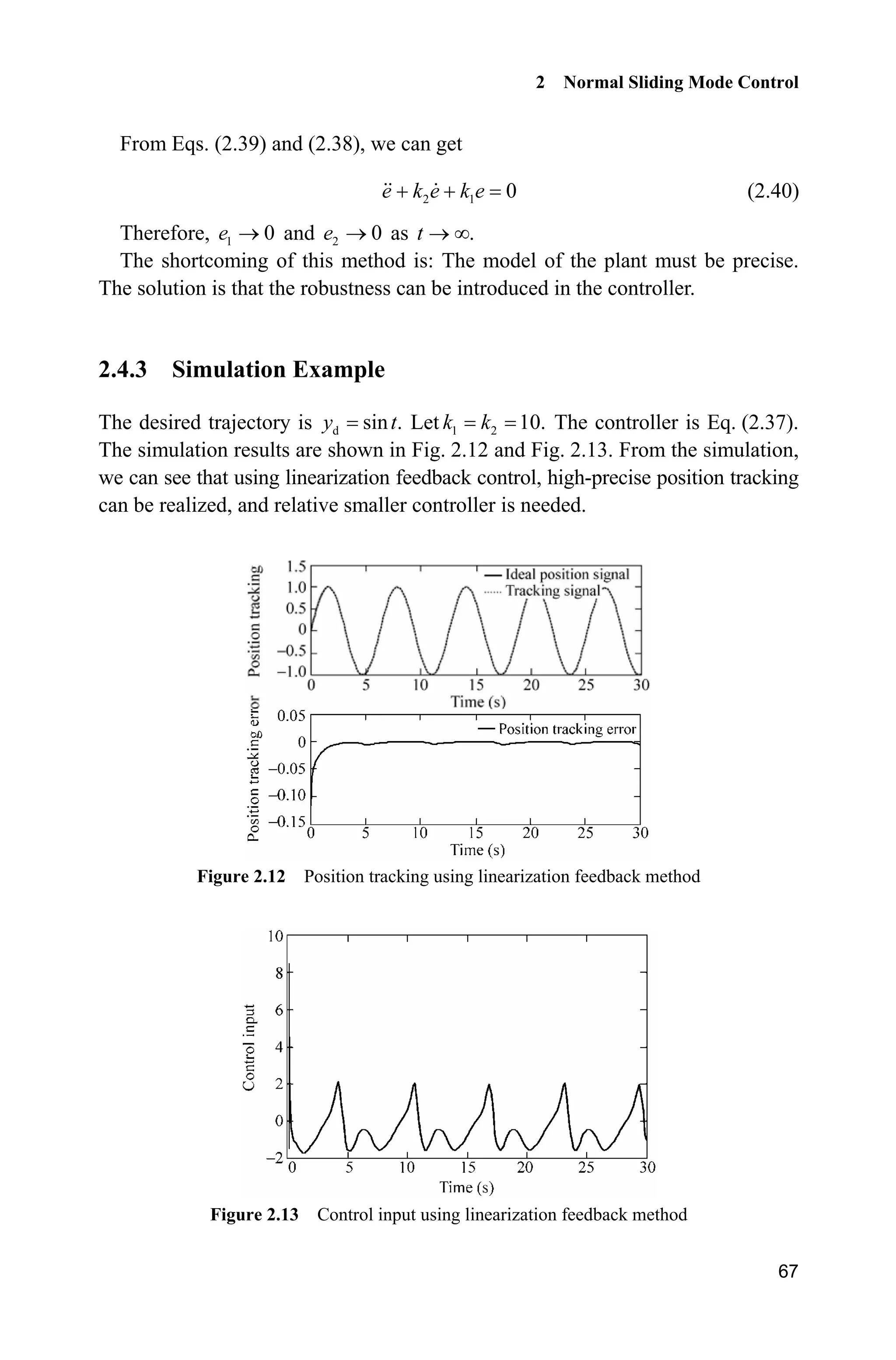
71
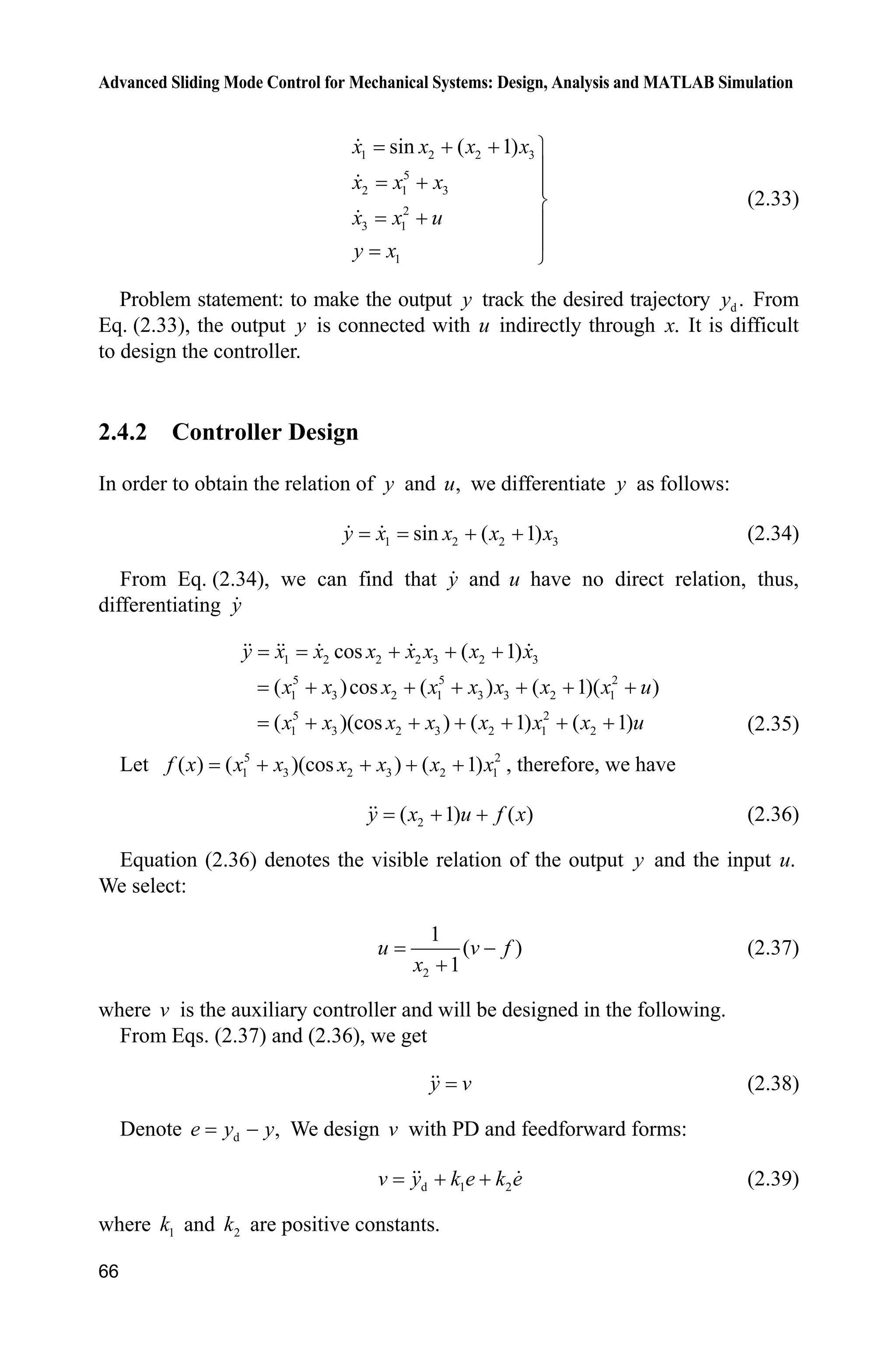
1 2 2 3 1sin ( 1)y x x x x d (2.42)
From Eq. (2.42), we can find that y and u have no direct relation, thus,
differentiate :y
1 2 2 2 3 2 3 1
5 5 2
1 3 2 2 1 3 2 3 2 1 3 1
5 2
1 3 2 3 2 1 2
cos ( 1)
( )cos ( ) ( 1)( )
( )(cos ) ( 1) ( 1)
y x x x x x x x d
x x d x x x d x x x u d d
x x x x x x x u d
(2.43)
where 2 2 2 3 2 3 1cos ( 1) .d d x d x x d d We assume | | .d D
Let 5 2
1 3 2 3 2 1( ) ( )(cos ) ( 1) ,f x x x x x x x therefore, equation (2.43) can be
transferred to
2( 1) ( )y x u f x d (2.44)
Denote d ,e y y and the sliding variable is selected as
( , )s x t ce (2.45)
where [ 1],cc 0,c ! T
[ ] .e ee
Equation (2.44)denotes the visible relation of the output y and the input .u
We select:
2
1
( sgn( ))
1
u v f s
x
K
(2.46)
where v is the auxiliary controller and will be designed in the following. .DK
Select Lyapunov function as
21
2
V s
We have
d
d 2
( ) ( )
( ( 1) ( ) )
V ss s e ce s y y ce
s y x u f x d ce
From Eq. (2.46), we have
d
d
( ( ( ) sgn( )) ( ) )
( ( ) sgn( ) ( ) )
V s y v f x s f x d ce
s y v f x s f x d ce
K
K
(2.47)
Select v be
dv y ce (2.48)](https://image.slidesharecdn.com/advancedslidingmodecontrolformechanicalsystems-130611121131-phpapp01/75/Advanced-sliding-mode-control-for-mechanical-systems-85-2048.jpg)
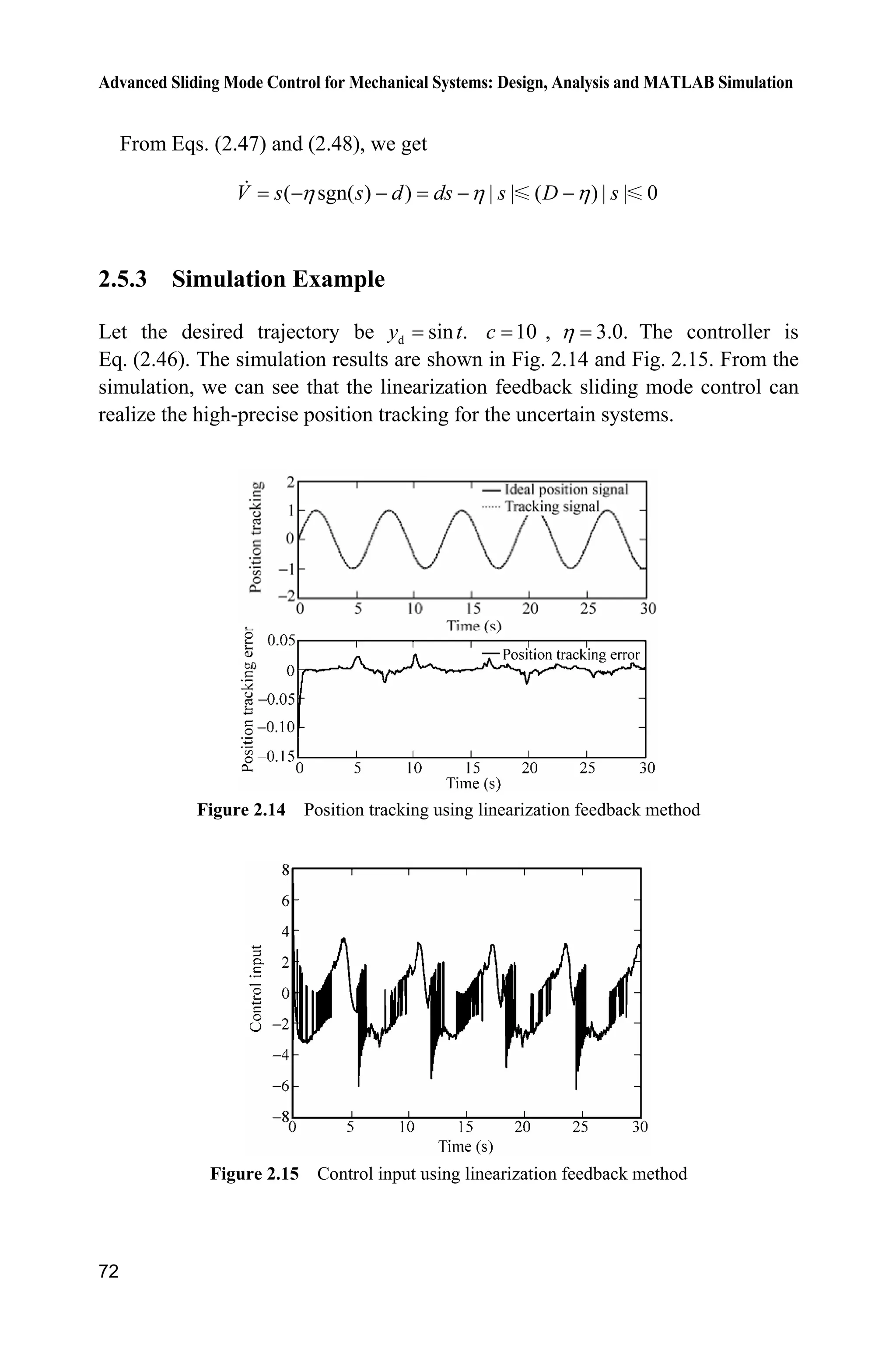
![2 Normal Sliding Mode Control
73
Simulation programs:
(1) Simulink main program: chap2_6sim.mdl
(2) Controller program: chap2_6ctrl.m
function [sys,x0,str,ts]=obser(t,x,u,flag)
switch flag,
case 0,
[sys,x0,str,ts]=mdlInitializeSizes;
case 1,
sys=mdlDerivatives(t,x,u);
case 3,
sys=mdlOutputs(t,x,u);
case {1, 2, 4, 9 }
sys = [];
otherwise
error(['Unhandled flag = ',num2str(flag)]);
end
function [sys,x0,str,ts]=mdlInitializeSizes
sizes = simsizes;
sizes.NumDiscStates = 0;
sizes.NumOutputs = 1;
sizes.NumInputs = 6;
sizes.DirFeedthrough = 1;
sizes.NumSampleTimes = 0;
sys=simsizes(sizes);
x0=[];
str=[];
ts=[];
function sys=mdlOutputs(t,x,u)
yd=u(1);
dyd=cos(t);
ddyd=-sin(t);](https://image.slidesharecdn.com/advancedslidingmodecontrolformechanicalsystems-130611121131-phpapp01/75/Advanced-sliding-mode-control-for-mechanical-systems-87-2048.jpg)
![Advanced Sliding Mode Control for Mechanical Systems: Design, Analysis and MATLAB Simulation
74
e=u(2);
de=u(3);
x1=u(4);
x2=u(5);
x3=u(6);
f=(x1^5+x3)*(x3+cos(x2))+(x2+1)*x1^2;
c=10;
s=de+c*e;
v=ddyd+c*de;
xite=3.0;
ut=1.0/(x2+1)*(v-f+xite*sign(s));
sys(1)=ut;
(3) The program of the plant: chap2_6plant.m
function [sys,x0,str,ts]=obser(t,x,u,flag)
switch flag,
case 0,
[sys,x0,str,ts]=mdlInitializeSizes;
case 1,
sys=mdlDerivatives(t,x,u);
case 3,
sys=mdlOutputs(t,x,u);
case {2, 4, 9 }
sys = [];
otherwise
error(['Unhandled flag = ',num2str(flag)]);
end
function [sys,x0,str,ts]=mdlInitializeSizes
sizes = simsizes;
sizes.NumContStates = 3;
sizes.NumDiscStates = 0;
sizes.NumOutputs = 3;
sizes.NumInputs = 1;
sizes.DirFeedthrough = 1;
sizes.NumSampleTimes = 0;
sys=simsizes(sizes);
x0=[0.15 0 0];
str=[];
ts=[];
function sys=mdlDerivatives(t,x,u)
ut=u(1);
d1=sin(t);
d2=sin(t);
d3=sin(t);
sys(1)=sin(x(2))+(x(2)+1)*x(3)+d1;
sys(2)=x(1)^5+x(3)+d2;
sys(3)=x(1)^2+ut+d3;
function sys=mdlOutputs(t,x,u)](https://image.slidesharecdn.com/advancedslidingmodecontrolformechanicalsystems-130611121131-phpapp01/75/Advanced-sliding-mode-control-for-mechanical-systems-88-2048.jpg)
![2 Normal Sliding Mode Control
75
sys(1)=x(1);
sys(2)=x(2);
sys(3)=x(3);
(4) Plot program: chap2_6plot.m
close all;
figure(1);
subplot(211);
plot(t,y(:,1),'k',t,y(:,2),'r:','linewidth',2);
xlabel('time(s)');ylabel('Position tracking');
legend('Ideal position signal','tracking signal');
subplot(212);
plot(t,y(:,1)-y(:,2),'k','linewidth',2);
xlabel('time');ylabel('position tracking error');
legend('position tracking error');
figure(2);
plot(t,ut(:,1),'k','linewidth',2);
xlabel('time');ylabel('control input');
2.6 Sliding Mode Control Based on Low Pass Filter
2.6.1 System Description
Consider the following second servo system:
( )J d tT W (2.49)
where J is the initial moment, W is the control input, ( )d t is the disturbance.
2.6.2 Sliding Mode Controller Design
Sliding mode control system with low pass filter is shown in Fig. 2.16.
Figure 2.16 Sliding mode control system with low pass filter
In Fig. 2.16, ( )u t is the virtual control input and ( )tW is the practical control
input. To decrease control chattering, low pass filter is designed as[2]](https://image.slidesharecdn.com/advancedslidingmodecontrolformechanicalsystems-130611121131-phpapp01/75/Advanced-sliding-mode-control-for-mechanical-systems-89-2048.jpg)
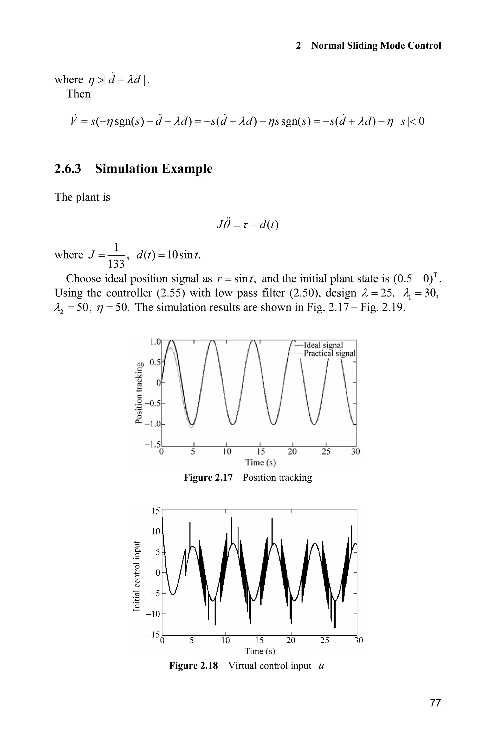
![Advanced Sliding Mode Control for Mechanical Systems: Design, Analysis and MATLAB Simulation
78
Figure 2.19 Practical control input W
Simulation programs:
(1) Main Simulink program: chap2_7sim.mdl
(2) Control law program: chap2_7ctrl.m
function [sys,x0,str,ts] = spacemodel(t,x,u,flag)
switch flag,
case 0,
[sys,x0,str,ts]=mdlInitializeSizes;
case 3,
sys=mdlOutputs(t,x,u);
case {2,4,9}
sys=[];
otherwise
error(['Unhandled flag = ',num2str(flag)]);
end
function [sys,x0,str,ts]=mdlInitializeSizes](https://image.slidesharecdn.com/advancedslidingmodecontrolformechanicalsystems-130611121131-phpapp01/75/Advanced-sliding-mode-control-for-mechanical-systems-92-2048.jpg)
![2 Normal Sliding Mode Control
79
sizes = simsizes;
sizes.NumContStates = 0;
sizes.NumDiscStates = 0;
sizes.NumOutputs = 1;
sizes.NumInputs = 5;
sizes.DirFeedthrough = 1;
sizes.NumSampleTimes = 1;
sys = simsizes(sizes);
x0 = [];
str = [];
ts = [0 0];
function sys=mdlOutputs(t,x,u)
tol=u(1);
th=u(2);
d_th=u(3);
dd_th=u(5);
J=10;
thd=sin(t);
d_thd=cos(t);
dd_thd=-sin(t);
ddd_thd=-cos(t);
e=th-thd;
de=d_th-d_thd;
dde=dd_th-dd_thd;
n1=30;n2=30;
n=25;
s=dde+n1*de+n2*e;
xite=80; %dot(d)+n*dmax,dmax=3
ut=-1/n*(-n*J*dd_th+J*(-ddd_thd+n1*dde+n2*de)+xite*sign(s));
sys(1)=ut;
(3) Plant S function: chap2_7plant.m
function [sys,x0,str,ts] = spacemodel(t,x,u,flag)
switch flag,
case 0,
[sys,x0,str,ts]=mdlInitializeSizes;
case 1,
sys=mdlDerivatives(t,x,u);
case 3,
sys=mdlOutputs(t,x,u);
case {2,4,9}
sys=[];
otherwise
error(['Unhandled flag = ',num2str(flag)]);
end](https://image.slidesharecdn.com/advancedslidingmodecontrolformechanicalsystems-130611121131-phpapp01/75/Advanced-sliding-mode-control-for-mechanical-systems-93-2048.jpg)
![Advanced Sliding Mode Control for Mechanical Systems: Design, Analysis and MATLAB Simulation
80
function [sys,x0,str,ts]=mdlInitializeSizes
sizes = simsizes;
sizes.NumContStates = 2;
sizes.NumDiscStates = 0;
sizes.NumOutputs = 2;
sizes.NumInputs = 1;
sizes.DirFeedthrough = 1;
sizes.NumSampleTimes = 1; % At least one sample time is needed
sys = simsizes(sizes);
x0 = [0.5;0];
str = [];
ts = [0 0];
function sys=mdlDerivatives(t,x,u) %Time-varying model
J=10;
ut=u(1);
d=3.0*sin(t);
sys(1)=x(2);
sys(2)=1/J*(ut-d);
function sys=mdlOutputs(t,x,u)
sys(1)=x(1);
sys(2)=x(2);
(4) Plot program: chap2_7plot.m
close all;
figure(1);
plot(t,y(:,1),'k',t,y(:,2),'r:','linewidth',2);
xlabel('time(s)');ylabel('Position tracking');
legend('ideal signal','practical signal');
figure(2);
plot(t,u,'k','linewidth',2);
xlabel('time(s)');ylabel('initial control input');
figure(3);
plot(t,tol,'k','linewidth',2);
xlabel('time(s)');ylabel('practical control input');
References
[1] Choi HS, Park YH, Cho Y, Lee M. Global sliding mode control. IEEE Control Magazine,
2001, 21(3): 27 35
[2] Kang BP, Ju JL. Sliding mode controller with filtered signal for robot manipulators using
virtual plant/controller, Mechatronics, 1997, 7(3): 277 286](https://image.slidesharecdn.com/advancedslidingmodecontrolformechanicalsystems-130611121131-phpapp01/75/Advanced-sliding-mode-control-for-mechanical-systems-94-2048.jpg)
![3 Advanced Sliding Mode Control
83
Therefore, we have
T T
f 0 0(| | ) | | ( ) | |V ss s f t sG H H B PB B PB
3.1.3 Sliding Mode Control Based on Auxiliary Feedback
In order to solve for symmetric positive-definite matrix P, the controller is
designed as[1,2]
( ) ( )u t v t Kx (3.7)
where eq n( ) .v t u u Kx
There exists K such that A A BK is stable, therefore, we have
( ) ( ) ( ( ))t t v f t x Ax B (3.8)
where K is a 1u4 vector, P, A and A are 4u4 matrixes, and B is a 4u1 vector.
Select the Lyapunov function as
T
V x Px (3.9)
Therefore,
T T
T T
2 2 ( ( ) ( ( )))
2 ( ) 2 ( ( ))
V t v f t
t v f t
x Px x P Ax B
x PAx x PB
When 0t t , there exists T
( ) 0s tB Px , i.e. T T
0s x PB , such that
T T T T
2 ( ) 2V x PAx x PA A P x x Mx
In order to satisfy 0,V 0M is needed, i.e.
T
0 PA A P
Since A is Hurwitz, then T
0 PA A P can be guaranteed[3]
.
Multiplying 1
P in the above inequality, we have
1 1 T
0
AP P A
Let 1
,
X P we get
T
0 AX XA
T
( ) ( ) 0 A BK X X A BK
Select ,L KX we have
T T T
0 AX BL XA L B (3.10)
In LMI, to guarantted P as symmetrical matrix, we design
T
P P or T
X X (3.11)](https://image.slidesharecdn.com/advancedslidingmodecontrolformechanicalsystems-130611121131-phpapp01/75/Advanced-sliding-mode-control-for-mechanical-systems-97-2048.jpg)
![3 Advanced Sliding Mode Control
85
Figure 3.2 Control input
Figure 3.3 Sliding variable
Simulation programs:
(1) Program of LMI design: chap3_lmi.m
clear all;
close all;
g=9.8;M=1.0;m=0.1;L=0.5;
I=1/12*m*L^2;
l=1/2*L;
t1=m*(M+m)*g*l/[(M+m)*I+M*m*l^2];
t2=-m^2*g*l^2/[(m+M)*I+M*m*l^2];
t3=-m*l/[(M+m)*I+M*m*l^2];
t4=(I+m*l^2)/[(m+M)*I+M*m*l^2];
A=[0,1,0,0;
t1,0,0,0;
0,0,0,1;
t2,0,0,0];
B=[0;t3;0;t4];](https://image.slidesharecdn.com/advancedslidingmodecontrolformechanicalsystems-130611121131-phpapp01/75/Advanced-sliding-mode-control-for-mechanical-systems-99-2048.jpg)
![Advanced Sliding Mode Control for Mechanical Systems: Design, Analysis and MATLAB Simulation
86
% LMI Var Description
setlmis([]);
X = lmivar(1, [4 1]); % 1 - symmetric block diagonal, then P is symmetric
L = lmivar(2, [1 4]); % Define L is 1 row,4 column
% LMI
%First LMI
lmiterm([1 1 1 X], A, 1, 's'); % A*X+X'*A'0
lmiterm([-1 1 1 L], B, 1, 's'); % 0B*L+L'*B'
%Second LMI
lmiterm([-2 1 1 X], 1, 1); % 0X, then P is positive matrix
lmis=getlmis;
[tmin,xfeas] = feasp(lmis);
X = dec2mat(lmis,xfeas,X)
P=inv(X)
%Verify A_bar is Hurwitz
L = dec2mat(lmis,xfeas,L)
K=L*inv(X);
A_bar=A-B*K
eig(A_bar)
save Pfile A B P;
(2) Simulation program of continuous system
Simulink main program: chap3_1sim.mdl
Program of controller: chap3_1ctrl.m
function [sys,x0,str,ts] = spacemodel(t,x,u,flag)
switch flag,
case 0,
[sys,x0,str,ts]=mdlInitializeSizes;](https://image.slidesharecdn.com/advancedslidingmodecontrolformechanicalsystems-130611121131-phpapp01/75/Advanced-sliding-mode-control-for-mechanical-systems-100-2048.jpg)
![3 Advanced Sliding Mode Control
87
case 3,
sys=mdlOutputs(t,x,u);
case {2,4,9}
sys=[];
otherwise
error(['Unhandled flag = ',num2str(flag)]);
end
function [sys,x0,str,ts]=mdlInitializeSizes
sizes = simsizes;
sizes.NumContStates = 0;
sizes.NumDiscStates = 0;
sizes.NumOutputs = 2;
sizes.NumInputs = 4;
sizes.DirFeedthrough = 1;
sizes.NumSampleTimes = 1;
sys = simsizes(sizes);
x0 = [];
str = [];
ts = [0 0];
function sys=mdlOutputs(t,x,u)
g=9.8;M=1.0;m=0.1;L=0.5;
I=1/12*m*L^2;
l=1/2*L;
t1=m*(M+m)*g*l/[(M+m)*I+M*m*l^2];
t2=-m^2*g*l^2/[(m+M)*I+M*m*l^2];
t3=-m*l/[(M+m)*I+M*m*l^2];
t4=(I+m*l^2)/[(m+M)*I+M*m*l^2];
A=[0,1,0,0;
t1,0,0,0;
0,0,0,1;
t2,0,0,0];
B=[0;t3;0;t4];
% P is solved by LMI
P=[7.4496 1.2493 1.0782 1.1384;
1.2493 0.3952 0.2108 0.3252;
1.0782 0.2108 0.3854 0.2280;
1.1384 0.3252 0.2280 0.4286];
deltaf=0.30;
epc0=0.5;
x=[u(1) u(2) u(3) u(4)]';
s=B'*P*x;
ueq=-inv(B'*P*B)*B'*P*A*x;
M=2;
if M==1
un=-inv(B'*P*B)*(norm(B'*P*B)*deltaf+epc0)*sign(s);](https://image.slidesharecdn.com/advancedslidingmodecontrolformechanicalsystems-130611121131-phpapp01/75/Advanced-sliding-mode-control-for-mechanical-systems-101-2048.jpg)
![Advanced Sliding Mode Control for Mechanical Systems: Design, Analysis and MATLAB Simulation
88
elseif M==2 %Saturated function
delta=0.05;
kk=1/delta;
if abs(s)delta
sats=sign(s);
else
sats=kk*s;
end
un=-inv(B'*P*B)*(norm(B'*P*B)*deltaf+epc0)*sats;
end
ut=un+ueq;
sys(1)=ut;
sys(2)=s;
Program of the plant: chap3_1plant.m
function [sys,x0,str,ts] = spacemodel(t,x,u,flag)
switch flag,
case 0,
[sys,x0,str,ts]=mdlInitializeSizes;
case 1,
sys=mdlDerivatives(t,x,u);
case 3,
sys=mdlOutputs(t,x,u);
case {2,4,9}
sys=[];
otherwise
error(['Unhandled flag = ',num2str(flag)]);
end
function [sys,x0,str,ts]=mdlInitializeSizes
sizes = simsizes;
sizes.NumContStates = 4;
sizes.NumDiscStates = 0;
sizes.NumOutputs = 4;
sizes.NumInputs = 1;
sizes.DirFeedthrough = 0;
sizes.NumSampleTimes = 0;
sys = simsizes(sizes);
x0 =[-pi/3,0,5.0,0];
str = [];
ts = [];
function sys=mdlDerivatives(t,x,u)
g=9.8;M=1.0;m=0.1;L=0.5;
I=1/12*m*L^2;
l=1/2*L;
t1=m*(M+m)*g*l/[(M+m)*I+M*m*l^2];
t2=-m^2*g*l^2/[(m+M)*I+M*m*l^2];
t3=-m*l/[(M+m)*I+M*m*l^2];
t4=(I+m*l^2)/[(m+M)*I+M*m*l^2];
A=[0,1,0,0;](https://image.slidesharecdn.com/advancedslidingmodecontrolformechanicalsystems-130611121131-phpapp01/75/Advanced-sliding-mode-control-for-mechanical-systems-102-2048.jpg)
![3 Advanced Sliding Mode Control
89
t1,0,0,0;
0,0,0,1;
t2,0,0,0];
B=[0;t3;0;t4];
f=1*0.3*sin(t);
ut=u(1);
dx=A*x+B*(ut-f);
sys(1)=x(2);
sys(2)=dx(2);
sys(3)=x(4);
sys(4)=dx(4);
function sys=mdlOutputs(t,x,u)
sys(1)=x(1);
sys(2)=x(2);
sys(3)=x(3);
sys(4)=x(4);
Plot program: chap3_1plot.m
close all;
figure(1);
subplot(411);
plot(t,x(:,1),'r','linewidth',2);
xlabel('time(s)');ylabel('Angle response');
subplot(412);
plot(t,x(:,2),'r','linewidth',2);
xlabel('time(s)');ylabel('Angle speed response');
subplot(413);
plot(t,x(:,3),'r','linewidth',2);
xlabel('time(s)');ylabel('Cart position response');
subplot(414);
plot(t,x(:,4),'r','linewidth',2);
xlabel('time(s)');ylabel('Cart speed response');
figure(2);
plot(t,ut(:,1),'r','linewidth',2);
xlabel('time(s)');ylabel('Control input');
figure(3);
plot(t,s(:,1),'r','linewidth',2);
xlabel('time(s)');ylabel('Sliding mode');
(3) Simulation program of the discrete system Main program: chap3_2.m
%Single Link Inverted Pendulum Control: LMI
clear all;
close all;
global A B
load Pfile;
u_1=0;](https://image.slidesharecdn.com/advancedslidingmodecontrolformechanicalsystems-130611121131-phpapp01/75/Advanced-sliding-mode-control-for-mechanical-systems-103-2048.jpg)
![Advanced Sliding Mode Control for Mechanical Systems: Design, Analysis and MATLAB Simulation
90
xk=[-pi/6,0,5.0,0]; %Initial state
ts=0.02; %Sampling time
for k=1:1:1000
time(k)=k*ts;
Tspan=[0 ts];
para(1)=u_1;
para(2)=time(k);
[t,x]=ode45('chap3_2plant',Tspan,xk,[],para);
xk=x(length(x),:);
x1(k)=xk(1);
x2(k)=xk(2);
x3(k)=xk(3);
x4(k)=xk(4);
x=[x1(k) x2(k) x3(k) x4(k)]';
s(k)=B'*P*x;
deltaf=0.30;
epc0=0.5;
ueq(k)=-inv(B'*P*B)*B'*P*A*x;
M=2;
if M==1
un(k)=-inv(B'*P*B)*(norm(B'*P*B)*deltaf+epc0)*sign(s(k));
elseif M==2 %Saturated function
delta=0.05;
kk=1/delta;
if abs(s(k))delta
sats=sign(s(k));
else
sats=kk*s(k);
end
un(k)=-inv(B'*P*B)*(norm(B'*P*B)*deltaf+epc0)*sats;
end
u(k)=ueq(k)+un(k);
u_1=u(k);
end
figure(1);
subplot(411);
plot(time,x1,'k','linewidth',2); %Pendulum Angle
xlabel('time(s)');ylabel('Angle');
subplot(412);
plot(time,x2,'k','linewidth',2); %Pendulum Angle Rate
xlabel('time(s)');ylabel('Angle rate');
subplot(413);
plot(time,x3,'k','linewidth',2); %Car Position
xlabel('time(s)');ylabel('Cart position');
subplot(414);](https://image.slidesharecdn.com/advancedslidingmodecontrolformechanicalsystems-130611121131-phpapp01/75/Advanced-sliding-mode-control-for-mechanical-systems-104-2048.jpg)
![3 Advanced Sliding Mode Control
93
3.2.4 Simulation Example
Considering a one link inverted pendulum as follows:
1 2
2
1 2 1 1 c 1 c
2 2 2
1 c 1 c
sin cos sin /( ) cos /( )
(4/3 cos /( )) (4/3 cos /( ))
°
®
° ¯
x x
g x mlx x x m m x m m
x u
l m x m m l m x m m
where 1x and 2x are the oscillation angle and the oscillation rate respectively.
2
9.8 m/s ,g cm is the vehicle mass, c 1kg,m m is the mass of pendulum bar,
0.1kg,m l is one half of pendulum length, 0.5 m,l u is the control input.
The desired trajectory is d ( ) 0.1sin( ),x t tS control rule is Eq. (3.17), and select
1 35c and 2 15.c The initial state of the inverted pendulum is [ /60 0].S
Simulation results are shown in Fig. 3.4 and Fig. 3.5.
Figure 3.4 Position tracking
Figure 3.5 Control input](https://image.slidesharecdn.com/advancedslidingmodecontrolformechanicalsystems-130611121131-phpapp01/75/Advanced-sliding-mode-control-for-mechanical-systems-107-2048.jpg)
![Advanced Sliding Mode Control for Mechanical Systems: Design, Analysis and MATLAB Simulation
94
Simulation programs:
(1) Simulink main program: chap3_3sim.mdl
(2) S-function of controller: chap3_3ctrl.m
function [sys,x0,str,ts] = spacemodel(t,x,u,flag)
switch flag,
case 0,
[sys,x0,str,ts]=mdlInitializeSizes;
case 3,
sys=mdlOutputs(t,x,u);
case {2,4,9}
sys=[];
otherwise
error(['Unhandled flag = ',num2str(flag)]);
end
function [sys,x0,str,ts]=mdlInitializeSizes
global M V x0 fai
sizes = simsizes;
sizes.NumDiscStates = 0;
sizes.NumOutputs = 1;
sizes.NumInputs = 3;
sizes.DirFeedthrough = 1;
sizes.NumSampleTimes = 1;
sys = simsizes(sizes);
x0=[];
str = [];
ts = [0 0];
function sys=mdlOutputs(t,x,u)
c1=35;
c2=15;
r=u(1);
dr=0.1*pi*cos(pi*t);](https://image.slidesharecdn.com/advancedslidingmodecontrolformechanicalsystems-130611121131-phpapp01/75/Advanced-sliding-mode-control-for-mechanical-systems-108-2048.jpg)
![3 Advanced Sliding Mode Control
95
ddr=-0.1*pi^2*sin(pi*t);
x1=u(2);
x2=u(3);
g=9.8;mc=1.0;m=0.1;l=0.5;
S=l*(4/3-m*(cos(x1))^2/(mc+m));
fx=g*sin(x1)-m*l*x2^2*cos(x1)*sin(x1)/(mc+m);
fx=fx/S;
gx=cos(x1)/(mc+m);
gx=gx/S;
e1=x1-r;
de1=x2-dr;
s=x2+c1*e1-dr;
xite=0.010;
ut=(1/gx)*(-fx-c2*s-e1-c1*de1+ddr-xite*sign(s));
sys(1)=ut;
(3) The program of the plant: chap3_3plant.m
function [sys,x0,str,ts]=s_function(t,x,u,flag)
switch flag,
case 0,
[sys,x0,str,ts]=mdlInitializeSizes;
case 1,
sys=mdlDerivatives(t,x,u);
case 3,
sys=mdlOutputs(t,x,u);
case {2, 4, 9 }
sys = [];
otherwise
error(['Unhandled flag = ',num2str(flag)]);
end
function [sys,x0,str,ts]=mdlInitializeSizes
sizes = simsizes;
sizes.NumContStates = 2;
sizes.NumDiscStates = 0;
sizes.NumOutputs = 2;
sizes.NumInputs = 1;
sizes.DirFeedthrough = 0;
sizes.NumSampleTimes = 0;
sys=simsizes(sizes);
x0=[pi/60 0];
str=[];
ts=[];
function sys=mdlDerivatives(t,x,u)
g=9.8;mc=1.0;m=0.1;l=0.5;](https://image.slidesharecdn.com/advancedslidingmodecontrolformechanicalsystems-130611121131-phpapp01/75/Advanced-sliding-mode-control-for-mechanical-systems-109-2048.jpg)
![Advanced Sliding Mode Control for Mechanical Systems: Design, Analysis and MATLAB Simulation
96
S=l*(4/3-m*(cos(x(1)))^2/(mc+m));
fx=g*sin(x(1))-m*l*x(2)^2*cos(x(1))*sin(x(1))/(mc+m);
fx=fx/S;
gx=cos(x(1))/(mc+m);
gx=gx/S;
sys(1)=x(2);
sys(2)=fx+gx*u;
function sys=mdlOutputs(t,x,u)
sys(1)=x(1);
sys(2)=x(2);
(4) Plot program: chap3_3plot.m
close all;
figure(1);
subplot(211);
plot(t,y(:,1),'r',t,y(:,2),'k:','linewidth',2);
xlabel('time(s)');ylabel('Position tracking');
subplot(212);
plot(t,y(:,1)-y(:,2),'k','linewidth',2);
xlabel('time(s)');ylabel('Position tracking error');
figure(2);
plot(t,ut(:,1),'k','linewidth',2);
xlabel('time(s)');ylabel('Control input');
References
[1] Gouaisbaut F, Dambrine M, Richard JP. Robust control of delay systems: a sliding mode
control, design via LMI, Systems Control Letters 46 (2002): 219 230
[2] Qu SC. Sliding mode control theory and application for uncertain system, Huazhong Normal
University Press, 2008, 6 (In chinese)
[3] Khalil HK. Nonlinear Systems (third edition). Prentice Hall, 2002](https://image.slidesharecdn.com/advancedslidingmodecontrolformechanicalsystems-130611121131-phpapp01/75/Advanced-sliding-mode-control-for-mechanical-systems-110-2048.jpg)
![4 Discrete Sliding Mode Control
Jinkun Liu
Beijing University of Aeronautics and Astronautics
P.R.China
E-mail: ljk@buaa.edu.cn
Xinhua Wang
National University of Singapore
Singapore
E-mail: wangxinhua04@gmail.com
Abstract This chapter introduces discrete sliding mode controllers, including
a typical discrete sliding mode controller and a kind of discrete sliding mode
controller based on disturbance observer.
Keywords discrete sliding mode control, disturbance observer, stability
analysis
4.1 Discrete Sliding Mode Controller Design and Analysis
4.1.1 System Description
Consider the following uncertain system
( 1) ( ) ( ) ( ) ( ) ' k k u k kx A A x B f (4.1)
where x is system state, 2 2u
RA and 2 2u
' RA are matrix, 2 1u
RB is a vector,
u R is control input, 2 1
f u
R is a vector, T
[0 ] ,bB 0.b !
The uncertain term 'A and the perturbation term ( )f k satisfy the classical
matching conditions, i.e.
'A BA , f Bf (4.2)
Advanced Sliding Mode Control for Mechanical Systems
© Tsinghua University Press, Beijing and Springer-Verlag Berlin Heidelberg 201
J. Liu et al.,
2](https://image.slidesharecdn.com/advancedslidingmodecontrolformechanicalsystems-130611121131-phpapp01/75/Advanced-sliding-mode-control-for-mechanical-systems-111-2048.jpg)
![Advanced Sliding Mode Control for Mechanical Systems: Design, Analysis and MATLAB Simulation
98
Then, the system (4.1) can be described as
( 1) ( ) [ ( ) ( )] k k k kx Ax B u d (4.3)
where ( ) ( ) ( ).d k k kAx f
4.1.2 Controller Design and Analysis
The controller is designed as
T 1 T T
d( ) ( ) ( ( 1) ( ) ( ) sgn( ( )))u k k k qs k s kK
C B C x C Ax (4.4)
where K , q , c are positive constant values, c must be Hurwitz, T
[ 1] ,cC
0 1,q | | ,d D T
.D KC B
Stability analysis is given as follows: If the ideal position signal is d ( )x k then
the tracking error is d( ) ( ) ( ),e k x k x k then
T
T T
d
T T T T
d
T T T
d
T T
d
T
( 1)
( 1)
( 1) ( 1)
( ) ( ) ( ) ( 1)
( ) ( 1) ( ) ( ) sgn( ( ))
( ) ( 1)
( ) sgn( ( )) ( )
K
K
s k
e k
x k x k
k u k d k k
k k k qs k s k
d k k
qs k s k d k
C
C C
C Ax C B C B C x
C Ax C x C Ax
C B C x
C B (4.5)
Since T T
| ( ) | ,d k D K C B C B then T
( )d kK K C B , T T
( )D d k C B C B
T
,DC B and then we have T
( ) 0,d kK !C B T
( ) 0,d kK C B T
D C B
T
( ) 0d k !C B and T T
( ) 0.D d k C B C B
Four conditions are analyzed as follows:
(1) When T
( ) ,s k D KC B we have
Consider ( ) 0,s k ! 0 1,q T
( ) 0,d kK C B T T
( ) 0,D d k !C B C B then
T
( 1) ( ) ( 1) ( ) ( ) 0s k s k q s k d kK C B
T T T
T T T
( 1) ( ) ( 1) ( ) ( ) ( 1)( ) ( )
( ) ( ) 0
s k s k q s k d k q D d k
q D D d k
K K K
K
!
C B C B C B
C B C B C B
Then,](https://image.slidesharecdn.com/advancedslidingmodecontrolformechanicalsystems-130611121131-phpapp01/75/Advanced-sliding-mode-control-for-mechanical-systems-112-2048.jpg)
![Advanced Sliding Mode Control for Mechanical Systems: Design, Analysis and MATLAB Simulation
100
4.1.3 Simulation Example
Consider the plant
2
133
( )
25
G s
s s
The sampling time is chosen as 0.001 s. Considering disturbance, the discrete
system can be written as
( 1) ( ) ( ( ) ( ))k k u k d k x Ax B
where
1 0.001
,
0 0.9753
ª º
« »
¬ ¼
A
0.0001
,
0.1314
ª º
« »
¬ ¼
B and ( )d k is disturbance.
Using the control law Eq. (4.4), and assuming the disturbance as ( )d k
1.5sin ,t choosing the ideal position signal as d ( ) sin ,x k t and designing T
C
[15 1], 0.80,q 1.5.D The initial state is [0.15 0]. The term d ( 1)x k can
be received by extrapolation method. The simulation results are shown in
Fig. 4.1 Fig. 4.3.
Figure 4.1 Sine signal tracking
Figure 4.2 Control input](https://image.slidesharecdn.com/advancedslidingmodecontrolformechanicalsystems-130611121131-phpapp01/75/Advanced-sliding-mode-control-for-mechanical-systems-114-2048.jpg)
![4 Discrete Sliding Mode Control
101
Figure 4.3 Phase trajectory
Simulation programs: chap4_1.m
%VSS controller based on decoupled disturbance compensator
clear all;
close all;
ts=0.001;
a=25;
b=133;
sys=tf(b,[1,a,0]);
dsys=c2d(sys,ts,'z');
[num,den]=tfdata(dsys,'v');
A=[0,1;0,-a];
B=[0;b];
C=[1,0];
D=0;
%Change transfer function to discrete position equation
[A1,B1,C1,D1]=c2dm(A,B,C,D,ts,'z');
A=A1;
b=B1;
c=15;
Ce=[c,1];
q=0.80; %0q1
d_up=1.5;
eq=Ce*b*d_up+0.10; %eqabs(Ce*b*m/g);0eq/faiq1
x_1=[0.15;0];
s_1=0;
u_1=0;
d_1=0;ed_1=0;
r_1=0;r_2=0;dr_1=0;
for k=1:1:10000
time(k)=k*ts;](https://image.slidesharecdn.com/advancedslidingmodecontrolformechanicalsystems-130611121131-phpapp01/75/Advanced-sliding-mode-control-for-mechanical-systems-115-2048.jpg)
![Advanced Sliding Mode Control for Mechanical Systems: Design, Analysis and MATLAB Simulation
102
d(k)=1.5*sin(k*ts);
x=A*x_1+b*(u_1+d(k));
r(k)=sin(k*ts);
%Using Waitui method
dr(k)=(r(k)-r_1)/ts;
dr_1=(r_1-r_2)/ts;
r1(k)=2*r(k)-r_1;
dr1(k)=2*dr(k)-dr_1;
xd=[r(k);dr(k)];
xd1=[r1(k);dr1(k)];
e(k)=x(1)-r(k);
de(k)=x(2)-dr(k);
s(k)=c*e(k)+de(k);
u(k)=inv(Ce*b)*(Ce*xd1-Ce*A*x+q*s(k)-eq*sign(s(k)));
r_2=r_1;r_1=r(k);
dr_1=dr(k);
x_1=x;
s_1=s(k);
x1(k)=x(1);
x2(k)=x(2);
u_1=u(k);
end
figure(1);
plot(time,r,'k',time,x1,'r:','linewidth',2);
xlabel('time(s)');ylabel('Position tracking');
legend('Ideal position signal','tracking signal');
figure(2);
plot(time,u,'k','linewidth',2);
xlabel('time(s)');ylabel('u');
figure(3);
plot(e,de,'k',e,-Ce(1)*e,'r','linewidth',2);
xlabel('e');ylabel('de');
4.2 Discrete Sliding Mode Control Based on Disturbance
Observer
4.2.1 System Description
Consider the uncertain discrete system as follow:
( 1) ( ) ( ( ) ( ))k k u k d k x Ax B (4.8)](https://image.slidesharecdn.com/advancedslidingmodecontrolformechanicalsystems-130611121131-phpapp01/75/Advanced-sliding-mode-control-for-mechanical-systems-116-2048.jpg)
![4 Discrete Sliding Mode Control
103
where x is system state, 2 2u
A R is a matrix, 2 1u
B R is a vector, 2 1
u u
R is
control input, T
[0 ] , 0,b b d! B R is the disturbance.
Let the desired input command be d ( ),kx and the tracking error be ( )ke
d( ) ( ).k kx x The sliding variable is designed as
( ) ( )s k kCe (4.9)
where [ 1],cC 0.c !
4.2.2 Discrete Sliding Mode Control Based on Disturbance Observer
In this section, we introduce a typical sliding mode controller base on disturbance
observer, which was proposed by Eun et al[1]
.
For Eq. (4.8), the sliding mode controller consists of the sliding mode control
element and the disturbance compensation. The controller proposed by Eun et al. as[1]
s c( ) ( ) ( )u k u k u k (4.10)
where
T 1 T T
s d( ) ( ) ( ( 1) ( ) ( ) sgn( ( )))u k k k qs k s kK
C B C x C Ax
c
ˆ( ) ( )u k d k
The disturbance observer was proposed by Eun et al. as:
T 1ˆ ˆ( ) ( 1) ( ) ( ( ) ( 1) sgn( ( 1)))d k d k g s k qs k s kK
C B (4.11)
where ˆ( ) ( ) ( )d k d k d k , K , q , and g are positive constants.
From Eqs. (4.8) and (4.10), we have
T T T
d
T T
d
T T T
d
T T T
d
T
( 1) ( 1) ( 1) ( 1)
( ( ) ( ) ( )) ( 1)
( ) ( ( 1) ( ) ( )
ˆsgn( ( ))) ( ) ( ) ( 1)
( ) sgn( ( )) ( )
s k k k k
k u k d k k
k k k qs k
s k d k d k k
qs k s k d k
K
K
C e C x C x
C Ax B B C x
C Ax C x C Ax
C B C B C x
C B
(4.12)
From Eqs. (4.11) and (4.12), we can get
T 1
T 1 T
ˆ( 1) ( 1) ( 1)
ˆ( 1) ( ) ( ) ( ( 1) ( ) sgn( ( )))
( 1) ( ) ( ) ( ) ( ) ( )
( 1) ( ) (1 ) ( )
d k d k d k
d k d k g s k qs k s k
d k d k d k g d k
d k d k g d k
K
C B
C B C B
(4.13)](https://image.slidesharecdn.com/advancedslidingmodecontrolformechanicalsystems-130611121131-phpapp01/75/Advanced-sliding-mode-control-for-mechanical-systems-117-2048.jpg)
![Advanced Sliding Mode Control for Mechanical Systems: Design, Analysis and MATLAB Simulation
104
4.2.3 Convergent Analysis of Disturbance Observer
Theorem 1 proposed by Eun et al. as follows.
Theorem 1[1]
: For the disturbance observer Eq. (4.11) there exists a positive
constant m, if | ( 1) ( ) |d k d k m then 0k exists, and when 0k k! then ( )d k
/m g is satisfied where 0 1.g
Proof:
( )d k can be decomposed as
1 2( ) ( ) ( )d k d k d k
Let 1(0) 0,d we can get 2 (0) (0),d d and because
1 2( 1) ( 1) ( 1)d k d k d k
We let
1 1( 1) (1 ) ( ) ( 1) ( )d k g d k d k d k (4.14)
From Eq. (4.13), we have
2 2( 1) (1 ) ( )d k g d k (4.15)
Inductive method is used to prove the theorem. Firstly, we prove 1( ) /d k m g .
(1) When 0,k we get: 1(0) 0 / .d m g
(2) Suppose 1| ( ) | / ,d k m g and from Eq. (4.14)and 0 1,g we can get
when 1,k
1 1| ( 1) | (1 ) | ( ) | | ( 1) ( ) | (1 )
m m
d k g d k d k d k g m
g g
is satisfied. From the above two equations, we have
1| ( ) | / ,d k m g 0k
From Eq. (4.15) and 0 1 1,g we get
2 2 2 2( 1) (1 ) ( ) (1 ) | ( ) | | ( ) |d k g d k g d k d k
Therefore, 2 ( )d k is decreasing. And if there exists 0 ,kc when 0 ,k kc! then 2 ( )d k
is arbitrary small.
From the analysis above, we find that there exists 0 ,k when 0 ,k k! such that
1 2 1 2| ( ) | | ( ) ( ) | ( ) | ( ) |
m
d k d k d k d k d k
g](https://image.slidesharecdn.com/advancedslidingmodecontrolformechanicalsystems-130611121131-phpapp01/75/Advanced-sliding-mode-control-for-mechanical-systems-118-2048.jpg)
![4 Discrete Sliding Mode Control
105
4.2.4 Stability Analysis
Theorem 2 proposed by Eun et al. as follows.
Theorem 2[1]
: For controller Eq. (4.10), the system is stable if the following
conditions are satisfied:
(1) 0 1,q 0 1;g
(2) There exists a positive constant m, | ( 1) ( ) | ;d k d k m
(3) T
0 .
m
g
K C B
Proof: Let T
( ) ( ),v k d kC B we have
T
| ( ) | ,
m
v k
g
K C B i.e. ( ) ,v kK K T T
( )
m m
v k
g g
C B C B
Equation (4.12)can be written as
( 1) ( ) sgn( ( )) ( )s k qs k s k v kK
The following four cases are discussed:
(1) When T
( ) 0,
m
s k
g
K !C B we have
( 1) ( ) ( 1) ( ) ( ) 0s k s k q s k v kK
T
T T
( 1) ( ) ( 1) ( ) ( ) ( 1) ( )
( ) 0
m
s k s k q s k v k q v k
g
m m
q v k
g g
K K K
K
§ ·
¨ ¸
© ¹
§ ·
!¨ ¸
© ¹
C B
C B C B
Therefore,
2 2
( 1) ( )s k s k
(2) When T
( ) 0,
m
s k
g
K C B we have
( 1) ( ) ( 1) ( ) ( ) 0s k s k q s k v kK !
T T
( 1) ( ) ( 1) ( ) ( ) ( ) ( )
( ) ( ) 0
s k s k q s k v k s k v k
m m
v k v k
g g
K K
K K
C B C B](https://image.slidesharecdn.com/advancedslidingmodecontrolformechanicalsystems-130611121131-phpapp01/75/Advanced-sliding-mode-control-for-mechanical-systems-119-2048.jpg)
![4 Discrete Sliding Mode Control
107
sufficiently small. If m and g are selected such that 1,
m
g
and because
T
,
m
g
KC B K is selected sufficiently small and make T
1.
m
g
KC B Therefore,
the convergence of ( 1)s k can be realized.
4.2.5 Simulation Example
Consider the plant as follows:
2
133
( )
25
G s
s s
The sampling time is 0.001 s. The discretization equation of the plant is after
factoring disturbance is
( 1) ( ) ( ( ) ( ))k k u k d k x Ax B
where
1 0.001
,
0 0.9753
ª º
« »
¬ ¼
A
0.0001
,
0.1314
ª º
« »
¬ ¼
B ( )d k is disturbance, and ( )d k
1.5sin(2 ).tS
Let the desired command be d ( ) sin ,x k t and use the control law (4.10).
Therefore, according to linear extrapolation method, we get d ( 1)x k
d d2 ( ) ( 1).x k x k The controller parameters are T
[15 1],C 0.80,q g
0.95, 0.01,m T
0.001.
m
g
K C B The initial state vector is [0.5 0]. The
simulation results are shown in Fig. 4.4 Fig. 4.7.
Figure 4.4 Sine tracking](https://image.slidesharecdn.com/advancedslidingmodecontrolformechanicalsystems-130611121131-phpapp01/75/Advanced-sliding-mode-control-for-mechanical-systems-121-2048.jpg)
![Advanced Sliding Mode Control for Mechanical Systems: Design, Analysis and MATLAB Simulation
108
Figure 4.5 Observation of disturbance
Figure 4.6 Control input
Figure 4.7 Phase trajectory
Simulation program:
chap4_2.m
%SMC controller based on decoupled disturbance compensator
clear all;
close all;
ts=0.001;
a=25;b=133;
sys=tf(b,[1,a,0]);](https://image.slidesharecdn.com/advancedslidingmodecontrolformechanicalsystems-130611121131-phpapp01/75/Advanced-sliding-mode-control-for-mechanical-systems-122-2048.jpg)
![4 Discrete Sliding Mode Control
109
dsys=c2d(sys,ts,'z');
[num,den]=tfdata(dsys,'v');
A0=[0,1;0,-a];
B0=[0;b];
C0=[1,0];
D0=0;
%Change transfer function to discrete position xiteuation
[A1,B1,C1,D1]=c2dm(A0,B0,C0,D0,ts,'z');
A=A1;
B=B1;
c=15;
C=[c,1];
q=0.80; %0q1
g=0.95;
m=0.010; %mabs(d(k+1)-d(k))
xite=C*B*m/g+0.0010; %xiteabs(C*B*m/g);0xite/faiq1
x_1=[0.5;0];
s_1=0;
u_1=0;
d_1=0;ed_1=0;
xd_1=0;xd_2=0;dxd_1=0;
for k=1:1:10000
time(k)=k*ts;
d(k)=1.5*sin(2*pi*k*ts);
d_1=d(k);
x=A*x_1+B*(u_1+d(k));
xd(k)=sin(k*ts);
dxd(k)=(xd(k)-xd_1)/ts;
dxd_1=(xd_1-xd_2)/ts;
xd1(k)=2*xd(k)-xd_1; %Using Waitui method
dxd1(k)=2*dxd(k)-dxd_1;
Xd=[xd(k);dxd(k)];
Xd1=[xd1(k);dxd1(k)];
e(k)=x(1)-Xd(1);
de(k)=x(2)-Xd(2);
s(k)=C*(x-Xd);
ed(k)=ed_1+inv(C*B)*g*(s(k)-q*s_1+xite*sign(s_1));
u(k)=-ed(k)+inv(C*B)*(C*Xd1-C*A*x+q*s(k)-xite*sign(s(k)));](https://image.slidesharecdn.com/advancedslidingmodecontrolformechanicalsystems-130611121131-phpapp01/75/Advanced-sliding-mode-control-for-mechanical-systems-123-2048.jpg)
![Advanced Sliding Mode Control for Mechanical Systems: Design, Analysis and MATLAB Simulation
110
xd_2=xd_1;xd_1=xd(k);
dxd_1=dxd(k);
ed_1=ed(k);
x_1=x;
s_1=s(k);
x1(k)=x(1);
x2(k)=x(2);
u_1=u(k);
end
figure(1);
plot(time,xd,'k',time,x1,'r:','linewidth',2);
xlabel('time(s)');ylabel('Position tracking');
legend('Ideal position signal','tracking signal');
figure(2);
plot(time,d,'k',time,ed,'r:','linewidth',2);
xlabel('time(s)');ylabel('d,ed');
legend('Practical d','Estimation d');
figure(3);
plot(time,u,'r','linewidth',2);
xlabel('time(s)');ylabel('Control input');
figure(4);
plot(e,de,'b',e,-C(1)*e,'r');
xlabel('e');ylabel('de');
Reference
[1] Yongsoon Eun, Jung-Ho Kim, Kwangsoo Kim, Dong-ll Cho, Discrete-time variable structure
controller with a decoupled disturbance compensator and its application to a CNC
servomechanism, IEEE Transactions on Control Systems Technology, 1999, 7(4): 414 423](https://image.slidesharecdn.com/advancedslidingmodecontrolformechanicalsystems-130611121131-phpapp01/75/Advanced-sliding-mode-control-for-mechanical-systems-124-2048.jpg)
![5 Dynamic Sliding Mode Control
Jinkun Liu
Beijing University of Aeronautics and Astronautics
P.R.China
E-mail: ljk@buaa.edu.cn
Xinhua Wang
National University of Singapore
Singapore
E-mail: wangxinhua04@gmail.com
Abstract This chapter introduces a kind of dynamic sliding mode controller
design, stability analysis and simulation examples are given.
Keywords dynamic sliding mode control, stability analysis
5.1 Problem Statement
Dynamic sliding method is used to design a new switching function. Alternatively,
it is used to construct a switching s in the normal sliding mode into a new
switching function. The switching function is relative to the first-order or high-order
derivative in the control input. Also, it can shift the discontinuous items into the
first-order or high-order derivative in the control input[1]
. Accordingly, a continuous
dynamic sliding mode control rule is obtained and the chatting phenomenon can
be reduced sufficiently.
5.2 Dynamic Sliding Mode Control Based on Dynamic
Switching Functions
5.2.1 System Description
Consider a nonlinear system as under:
Advanced Sliding Mode Control for Mechanical Systems
© Tsinghua University Press, Beijing and Springer-Verlag Berlin Heidelberg 201
J. Liu et al.,
2](https://image.slidesharecdn.com/advancedslidingmodecontrolformechanicalsystems-130611121131-phpapp01/75/Advanced-sliding-mode-control-for-mechanical-systems-125-2048.jpg)
![Advanced Sliding Mode Control for Mechanical Systems: Design, Analysis and MATLAB Simulation
112
1 2
2
1
( ) ( ) ( )
x x
x f g u d t
y x
½
°
¾
°
¿
x x (5.1)
where 1 2 1[ ],x x xx and 2x are system states, y is output, ( )f x and ( )g x are
the known smoothing functions, ( )d t is uncertain, and 0| ( ) | ,d t D | ( ) | .d t D
5.2.2 Design of Controller
Define the tracking error and the switching function as de y y and s ce e
respectively. Where 0c ! must be Hurwitz. Therefore,
( ) ( ) ( ) ds f x g x u d t y ce (5.2)
Construct a new dynamic switching function as
s sV O (5.3)
where 0O ! must be Hurwitz.
When 0,V 0s sO is a asymptotically stable, therefore, 0e o and 0e o .
Stability analysis is given as follows: from Eq. (5.3), we have
( ) ( ) ( ) ds s f x g x u d t y ce sV O O
Therefore,
d
d
( ) ( ) ( ) ( )
( ) ( ) ( ) ( ) ( ( ) ( ) ( ) )
( ( ) ( ) ( ) )
( ) ( ) ( ) ( ) ( ) ( ( ) ( ) ( ))
( ) (
V O
O
O O O
O
d
d
d
d
f x g x u g x u d t y ce s
f x g x u g x u d t y c f x g x u d t y
f x g x u d t y ce
f x c y y d t c d t g x cg x g x u
c f x) ( ) O g x u ce (5.4)
Select the dynamic controller as
d
1
( ( ) ( ) ( ( ) ( )
( )
( )) ( ) ( ) sgn( ))
du f x c y y g x cg x
g x
g x u c f x ce
O
O O O K V
(5.5)
From Eqs. (5.5)and (5.4), we can get
( ) ( ) ( ) sgn( )d t c d tV O K V
Let 0( ) ,D c DK O! therefore,
0
( ( ) ( ) ( ) sgn( ))
( ( ) ( ) ( )) | | ( ( ) ) | | 0
d t c d t
d t c d t D c D
VV V O K V
V O K V O V K V](https://image.slidesharecdn.com/advancedslidingmodecontrolformechanicalsystems-130611121131-phpapp01/75/Advanced-sliding-mode-control-for-mechanical-systems-126-2048.jpg)
![5 Dynamic Sliding Mode Control
113
5.2.3 Simulation Example
Consider the time-variant system below:
1 2
2 225 133 3sin
x x
x x u t
where 2( ) 25 ,f x x ( ) 133,g x ( ) 3sin .d t t
Therefore, we have 0 3,D 3,D 2( ) 25 ,f x x ( ) 0.g x Then DK !
0( ) 3 (5 15) 3 63.c DO u
Let the desired trajectory be sin ,r t the tracking error is 1 .e x r Let
5,c 15,O The initial state vector is (0) [0.5 0].x The controller is shown
in Eq. (5.5), i.e.
d
1
( ( ) ( ) ( ) ( ) ( ) ( ) sgn( ))
( )
du f x c y y c g x u c f x ce
g x
O O O O K V
The simulation results are shown in Fig. 5.1 Fig. 5.3.
Figure 5.1 Position tracking
Figure 5.2 Dynamic controller u](https://image.slidesharecdn.com/advancedslidingmodecontrolformechanicalsystems-130611121131-phpapp01/75/Advanced-sliding-mode-control-for-mechanical-systems-127-2048.jpg)
![Advanced Sliding Mode Control for Mechanical Systems: Design, Analysis and MATLAB Simulation
114
Figure 5.3 Actual controller u
Simulation programs:
(1) Main program: chap5_1sim.mdl
(2) S-function: chap5_1ctrl.m
function [sys,x0,str,ts] = spacemodel(t,x,u,flag)
switch flag,
case 0,
[sys,x0,str,ts]=mdlInitializeSizes;
case 3,
sys=mdlOutputs(t,x,u);
case {2,4,9}
sys=[];
otherwise
error(['Unhandled flag = ',num2str(flag)]);
end
function [sys,x0,str,ts]=mdlInitializeSizes
sizes = simsizes;
sizes.NumContStates = 0;
sizes.NumDiscStates = 0;
sizes.NumOutputs = 2;](https://image.slidesharecdn.com/advancedslidingmodecontrolformechanicalsystems-130611121131-phpapp01/75/Advanced-sliding-mode-control-for-mechanical-systems-128-2048.jpg)
![5 Dynamic Sliding Mode Control
115
sizes.NumInputs = 4;
sizes.DirFeedthrough = 1;
sizes.NumSampleTimes = 0;
sys = simsizes(sizes);
x0 = [];
str = [];
ts = [];
function sys=mdlOutputs(t,x,u)
x1=u(1);
dx1=u(2);
ddx1=u(3);
ut=u(4);
r=sin(t);
dr=cos(t);
ddr=-sin(t);
dddr=-cos(t);
e=x1-r;
de=dx1-dr;
dde=ddx1-ddr;
c=15;
s=c*e+de;
fx=-25*dx1;df=-25*ddx1;
gx=133;
nmn=15;
D0=3;D=3;
xite=D+(c+nmn)*D0+0.50;
ds=c*de+dde;
rou=ds+nmn*s;
du=1/gx*[-df+(c+nmn)*ddr+dddr-(c+nmn)*gx*ut-(c+nmn)*fx-nmn*c*de-xite*sign(
rou)];
sys(1)=r;
sys(2)=du;
(3) The program of the plant: chap5_1plant.m
function [sys,x0,str,ts]=s_function(t,x,u,flag)
switch flag,
case 0,
[sys,x0,str,ts]=mdlInitializeSizes;
case 1,
sys=mdlDerivatives(t,x,u);
case 3,
sys=mdlOutputs(t,x,u);
case {2, 4, 9 }
sys = [];](https://image.slidesharecdn.com/advancedslidingmodecontrolformechanicalsystems-130611121131-phpapp01/75/Advanced-sliding-mode-control-for-mechanical-systems-129-2048.jpg)
![Advanced Sliding Mode Control for Mechanical Systems: Design, Analysis and MATLAB Simulation
116
otherwise
error(['Unhandled flag = ',num2str(flag)]);
end
function [sys,x0,str,ts]=mdlInitializeSizes
sizes = simsizes;
sizes.NumContStates = 2;
sizes.NumDiscStates = 0;
sizes.NumOutputs = 1;
sizes.NumInputs = 1;
sizes.DirFeedthrough = 0;
sizes.NumSampleTimes = 0;
sys=simsizes(sizes);
x0=[0,0];
str=[];
ts=[];
function sys=mdlDerivatives(t,x,u)
dt=3*sin(t);
sys(1)=x(2);
sys(2)=-25*x(2)+133*u+dt;
function sys=mdlOutputs(t,x,u)
sys(1)=x(1);
(4) Plot program: chap5_1plot.m
close all;
figure(1);
plot(t,y(:,1),'k',t,y(:,2),'r:','linewidth',2);
xlabel('time(s)');ylabel('Position tracking');
legend('ideal signal','tracking signal');
figure(2);
plot(t,du(:,1),'r','linewidth',2);
xlabel('time(s)');ylabel('Derivative of Control input');
figure(3);
plot(t,u,'r','linewidth',2);
xlabel('time(s)');ylabel('Control input');
Reference
[1] Ramirez HS, Santiago OL. Adaptive dynamical sliding mode control via backstepping,
Proceedings of the 32th
Conference on Decision and Control, San Antonia, Texas, December,
1992, 1422 1427](https://image.slidesharecdn.com/advancedslidingmodecontrolformechanicalsystems-130611121131-phpapp01/75/Advanced-sliding-mode-control-for-mechanical-systems-130-2048.jpg)
![6 Adaptive Sliding Mode Control for Mechanical Systems
119
2
1 1 ˆ( )V ss s x qT TT T T TT
J J
Select the adaptive law as
ˆ qsT J (6.12)
Therefore,
2 2
s
1 ˆ( )
1ˆ( sgn( ) ) ( )
( sgn( ) ) ( )
| | 0
s
s
s
V s u q
s q k s s q qs
s q k s s qs
k s s s k s
' T TT
J
T K ' T T J
J
T K ' T
K '
˜
In order to avoid ˆT which is too big to make ( )u t too big, we rewrite Eq. (6.12)
by using the discontinuous projection mapping proposed in [1] as
ˆ
ˆ Proj ( )qsT
T J (6.13)
max
ˆ min
ˆ0, if and 0
ˆProj ( ) 0, if and 0
, otherwise
T
T T
T T
!
°°
®
°
°¯
˜
˜ ˜
˜
6.1.3 Simulation Example
The plant is
1
2
2
d
d
d
( )
d
x
x
t
x
m u t
t
'
where 1.0,m ' is the friction model and denoted as 0.5 1.5sign( ).' T T
The desired trajectory is selected as sint , and the range of the parameter T is
assumed as min 0.5T and max 1.5.T Choosing 15,c s 15,k 500J and
0.01 1.01.DK The adaptive sliding mode controller (6.7) is adopted (M 1).
If the adaptive law is selected as Eq. (6.12) (N 1), then the simulation results are
shown in Fig. 6.1 Fig. 6.3. If the adaptive law is selected as Eq. (6.13) (N 2), then
the simulation results are shown in Fig. 6.4 Fig. 6.6. By adopting the improved
adaptive law the range of T can be limited and a too big ( )u t is avoided.](https://image.slidesharecdn.com/advancedslidingmodecontrolformechanicalsystems-130611121131-phpapp01/75/Advanced-sliding-mode-control-for-mechanical-systems-133-2048.jpg)
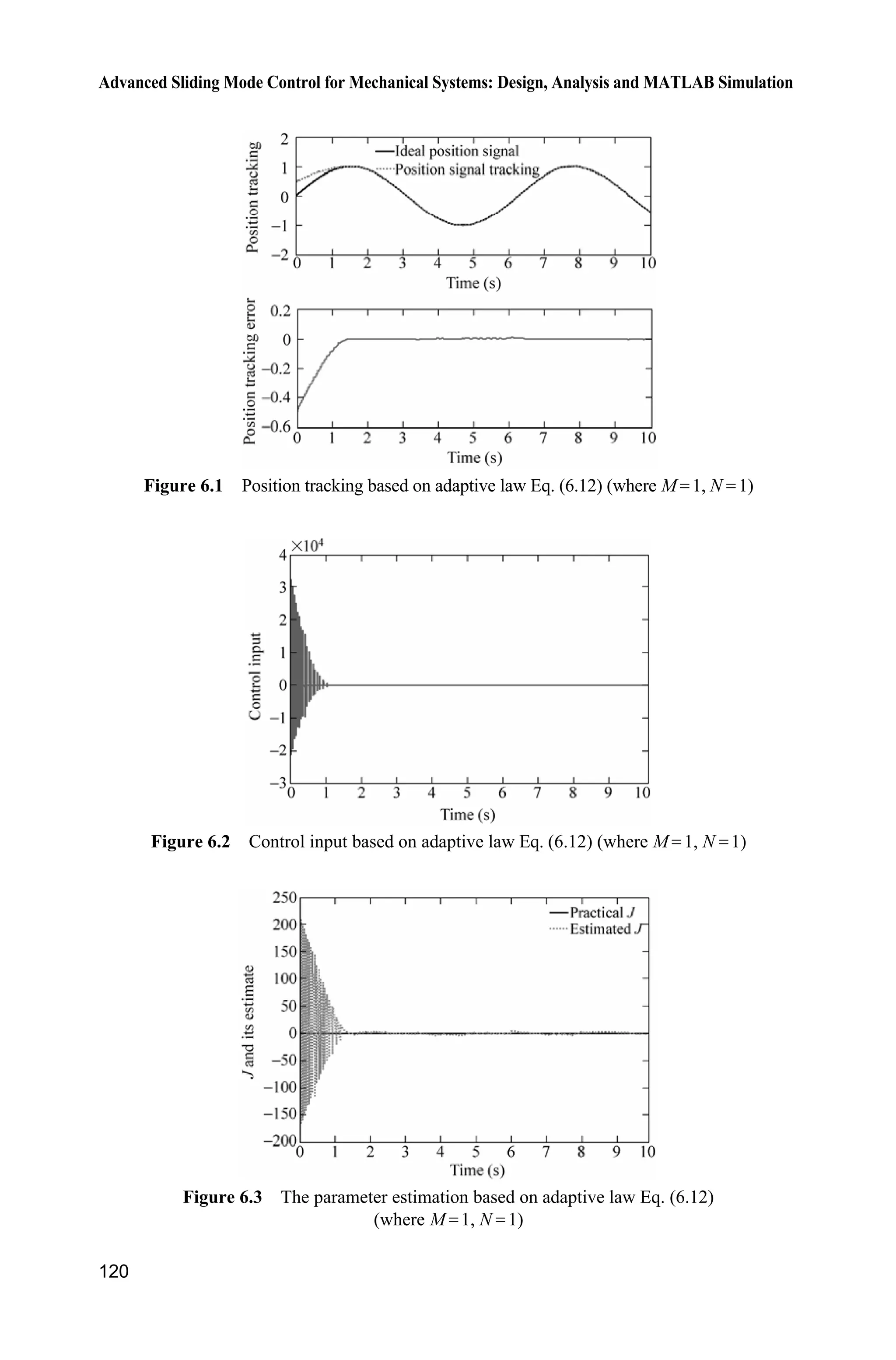
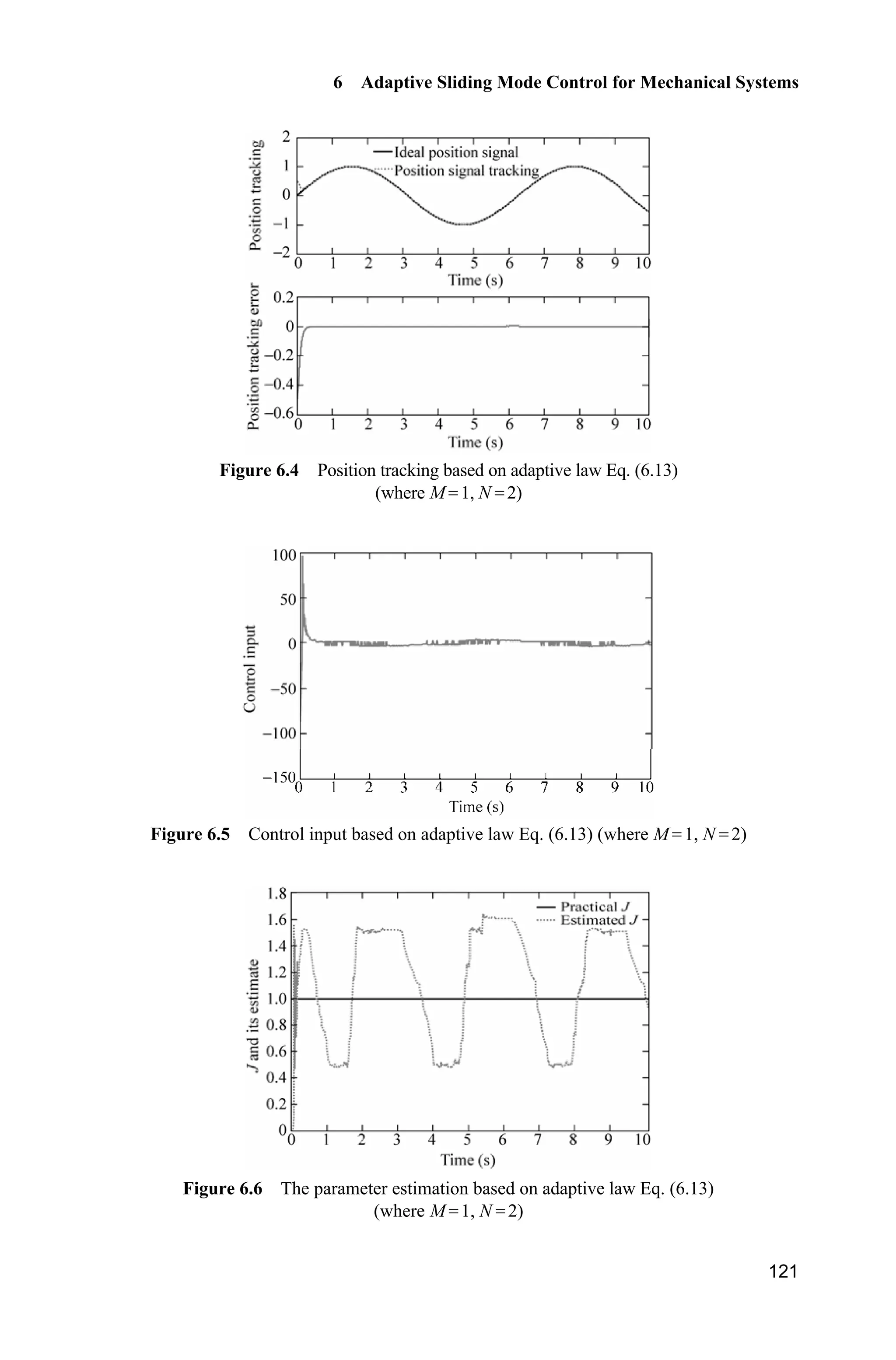
![Advanced Sliding Mode Control for Mechanical Systems: Design, Analysis and MATLAB Simulation
122
PD controller (M 2) is selected, and p d100, 50.k k The simulation result
is shown in Fig. 6.7. We can find that the flattop phenomenon happens and the
high precise tracking performance can be obtained.
Figure 6.7 Position tracking by PD controller (M 2)
In the adaptive control simulation, the parameter estimation error isn’t converged
to zero for the latter case, the reason can be explained that the tracking error
convergence can be achieved by many possible values of the estimated parameter
m, besides the true parameter m. Therefore, the parameter adaption law does not
bother to find out the ture parameter m[5]
.
Simulation programs:
(1) Main Simulink program: chap6_1sim.mdl
(2) Control law program: chap6_1ctrl.m
function [sys,x0,str,ts]=s_function(t,x,u,flag)
switch flag,](https://image.slidesharecdn.com/advancedslidingmodecontrolformechanicalsystems-130611121131-phpapp01/75/Advanced-sliding-mode-control-for-mechanical-systems-136-2048.jpg)
![6 Adaptive Sliding Mode Control for Mechanical Systems
123
case 0,
[sys,x0,str,ts]=mdlInitializeSizes;
case 3,
sys=mdlOutputs(t,x,u);
case {1,2, 4, 9 }
sys = [];
otherwise
error(['Unhandled flag = ',num2str(flag)]);
end
function [sys,x0,str,ts]=mdlInitializeSizes
sizes = simsizes;
sizes.NumContStates = 0;
sizes.NumDiscStates = 0;
sizes.NumOutputs = 1;
sizes.NumInputs = 3;
sizes.DirFeedthrough = 1;
sizes.NumSampleTimes = 1;
sys=simsizes(sizes);
x0=[];
str=[];
ts=[0 0];
function sys=mdlOutputs(t,x,u)
e=u(1);
de=u(2);
dxd=cos(t);
ddxd=-sin(t);
thp=u(3);
c=15;
s=de+c*e; %Sliding Mode
x2=dxd+de;
dq=ddxd-c*de;
ks=15;
xite=2.01;
ua=thp*dq;
us1=-ks*s;
us2=-xite*sign(s);
M=1;
if M==1 %DRC
ut=ua+us1+us2;
elseif M==2 %PD
kp=100;kd=50;
ut=-kp*e-kd*de;
end
sys(1)=ut;
(3) Plant S-function chap6_1plant.m
function [sys,x0,str,ts]=s_function(t,x,u,flag)
switch flag,](https://image.slidesharecdn.com/advancedslidingmodecontrolformechanicalsystems-130611121131-phpapp01/75/Advanced-sliding-mode-control-for-mechanical-systems-137-2048.jpg)
![Advanced Sliding Mode Control for Mechanical Systems: Design, Analysis and MATLAB Simulation
124
case 0,
[sys,x0,str,ts]=mdlInitializeSizes;
case 1,
sys=mdlDerivatives(t,x,u);
case 3,
sys=mdlOutputs(t,x,u);
case {2, 4, 9 }
sys = [];
otherwise
error(['Unhandled flag = ',num2str(flag)]);
end
function [sys,x0,str,ts]=mdlInitializeSizes
sizes = simsizes;
sizes.NumContStates = 2;
sizes.NumDiscStates = 0;
sizes.NumOutputs = 2;
sizes.NumInputs = 1;
sizes.DirFeedthrough = 1;
sizes.NumSampleTimes = 0;
sys=simsizes(sizes);
x0=[0.5;0];
str=[];
ts=[];
function sys=mdlDerivatives(t,x,u)
m=1.0;
ut=u(1);
F=0.5*x(2)+1.5*sign(x(2));
sys(1)=x(2);
sys(2)=1/m*(ut-F);
function sys=mdlOutputs(t,x,u)
m=1.0;
sys(1)=x(1);
sys(2)=m;
(4) Adapt S-function of drc chap6_1adapt.m
function [sys,x0,str,ts]=s_function(t,x,u,flag)
switch flag,
case 0,
[sys,x0,str,ts]=mdlInitializeSizes;
case 1,
sys=mdlDerivatives(t,x,u);
case 3,
sys=mdlOutputs(t,x,u);
case {2, 4, 9 }
sys = [];
otherwise
error(['Unhandled flag = ',num2str(flag)]);
end
function [sys,x0,str,ts]=mdlInitializeSizes
sizes = simsizes;](https://image.slidesharecdn.com/advancedslidingmodecontrolformechanicalsystems-130611121131-phpapp01/75/Advanced-sliding-mode-control-for-mechanical-systems-138-2048.jpg)
![6 Adaptive Sliding Mode Control for Mechanical Systems
125
sizes.NumContStates = 1;
sizes.NumDiscStates = 0;
sizes.NumOutputs = 1;
sizes.NumInputs = 2;
sizes.DirFeedthrough = 1;
sizes.NumSampleTimes = 0;
sys=simsizes(sizes);
x0=[0];
str=[];
ts=[];
function sys=mdlDerivatives(t,x,u)
e=u(1);
de=u(2);
dxd=cos(t);
ddxd=-sin(t);
x2=dxd+de;
c=15;
gama=500;
s=de+c*e;
thp=x(1);
dq=ddxd-c*de;
th_min=0.5;
th_max=1.5;
alaw=-gama*dq*s; %Adaptive law
N=2;
if N==1 %Adaptive law
sys(1)=alaw;
elseif N==2 %Adaptive law with Proj
if thp=th_maxalaw0
sys(1)=0;
elseif thp=th_minalaw0
sys(1)=0;
else
sys(1)=alaw;
end
end
function sys=mdlOutputs(t,x,u)
sys(1)=x(1); %m estimate
(5) Plot program: chap6_1plot.m
close all;
figure(1);
subplot(211);
plot(t,y(:,1),'k',t,y(:,2),'r:','linewidth',2);
xlabel('time(s)');ylabel('Position tracking');](https://image.slidesharecdn.com/advancedslidingmodecontrolformechanicalsystems-130611121131-phpapp01/75/Advanced-sliding-mode-control-for-mechanical-systems-139-2048.jpg)
![Advanced Sliding Mode Control for Mechanical Systems: Design, Analysis and MATLAB Simulation
126
legend('Ideal position signal','Position signal tracking');
subplot(212);
plot(t,y(:,1)-y(:,2),'r','linewidth',2);
xlabel('time(s)');ylabel('Position tracking error');
figure(2);
plot(t,ut(:,1),'r','linewidth',2);
xlabel('time(s)');ylabel('Control input');
figure(3);
plot(t,y(:,3),'k',t,p(:,1),'r:','linewidth',2);
xlabel('time(s)');ylabel('J and its estimate');
legend('Practical J','Estimated J');
6.2 Adaptive Sliding Mode Control of Inverted Pendulum
6.2.1 System Description
The kinetic equation of the inverted pendulum is given as follow:
1 2
2
1 p 2 1 1 c p 1 c p
2 2 2
p 1 c p p 1 c p
sin cos sin /( ) cos /( )
(4/3 cos /( )) (4/3 cos /( ))
x x
g x m lx x x m m x m m
x u
l m x m m l m x m m
½
°
¾
° ¿
(6.14)
where 1x and 2x are the pendulum angle T and pendulum speed T respectively,
u is control input, cm is the cart mass, pm is the pendulum mass, and l is the half
of pendulum length.
6.2.2 Control System Design
In order to realize the controller design for system (6.14) without modeling
information, we arrange Eq. (6.14) by using the methods proposed by Ebrahim
and Murphy[4]
as follows:
2 2
c p p 1 2 1 c p p 2 1 1 1(4/3( ) cos ) sin ( ) cos sin cosl m m m x x g x m m m lx x x x u
and
2
c p 1 p 1 2 1 c p p 2 1(4/3( )sec cos ) tan ( ) sinl m m x m x x g x m m m lx x u](https://image.slidesharecdn.com/advancedslidingmodecontrolformechanicalsystems-130611121131-phpapp01/75/Advanced-sliding-mode-control-for-mechanical-systems-140-2048.jpg)
![6 Adaptive Sliding Mode Control for Mechanical Systems
127
Since 2
p
1
,
3
I m l then
2
p
p
4
3
I m l
l
m l
and
2
p 2
c p 1 p 1 2 1 c p p 2 1
p
( )sec cos tan ( ) sin
I m l
m m x m l x x g x m m m lx x u
m l
§ ·
¨ ¸¨ ¸
© ¹
(6.15)
In order to design controller without need model information, we choose[4]
2
p
1 c p
p
( )
( ) ,I
˜
I m l
m m
m l
2 c p( ) ,m m gI 3 pm lI
Considering outer disturbance, we transfer Eq. (6.15) to state equation as
1 2
2
1 2 2 1 3 2 1( ) tan sin
x x
g x x u x x x dtI I
(6.16)
where 1 1 1 3 1( ) sec cos ,g x x xI I dt is the outer disturbance.
Define dT as the ideal position signal and 1 de x T as the position tracking
error. Then, the sliding function is ,s ce e 0.c !
The Lyapunov function is defined as
2 2 2 2
1 1 1 2 2 3 3
1 2 3
1 1 1 1ˆ ˆ ˆ( ) ( ) ( ) ( )
2 2 2 2
V g x s I I I I I I
J J J
(6.17)
where 0,iJ ! ˆ
iI is estimation value of ( 1,2,3).i iI
Choose 2
1 1
1
( ) ,
2
V g x s 2 2 2
2 1 1 2 2 3 3
1 2 3
1 1 1ˆ ˆ ˆ( ) ( ) ( ) ,
2 2 2
V I I I I I I
J J J
then
2
1 1 1
1
( ) ( )
2
V g x s g x ss
2 1 1 1 2 2 2 3 3 3
1 2 3
1 1 1ˆ ˆ ˆ ˆ ˆ ˆ( ) ( ) ( )V I I I I I I I I I
J J J
where](https://image.slidesharecdn.com/advancedslidingmodecontrolformechanicalsystems-130611121131-phpapp01/75/Advanced-sliding-mode-control-for-mechanical-systems-141-2048.jpg)
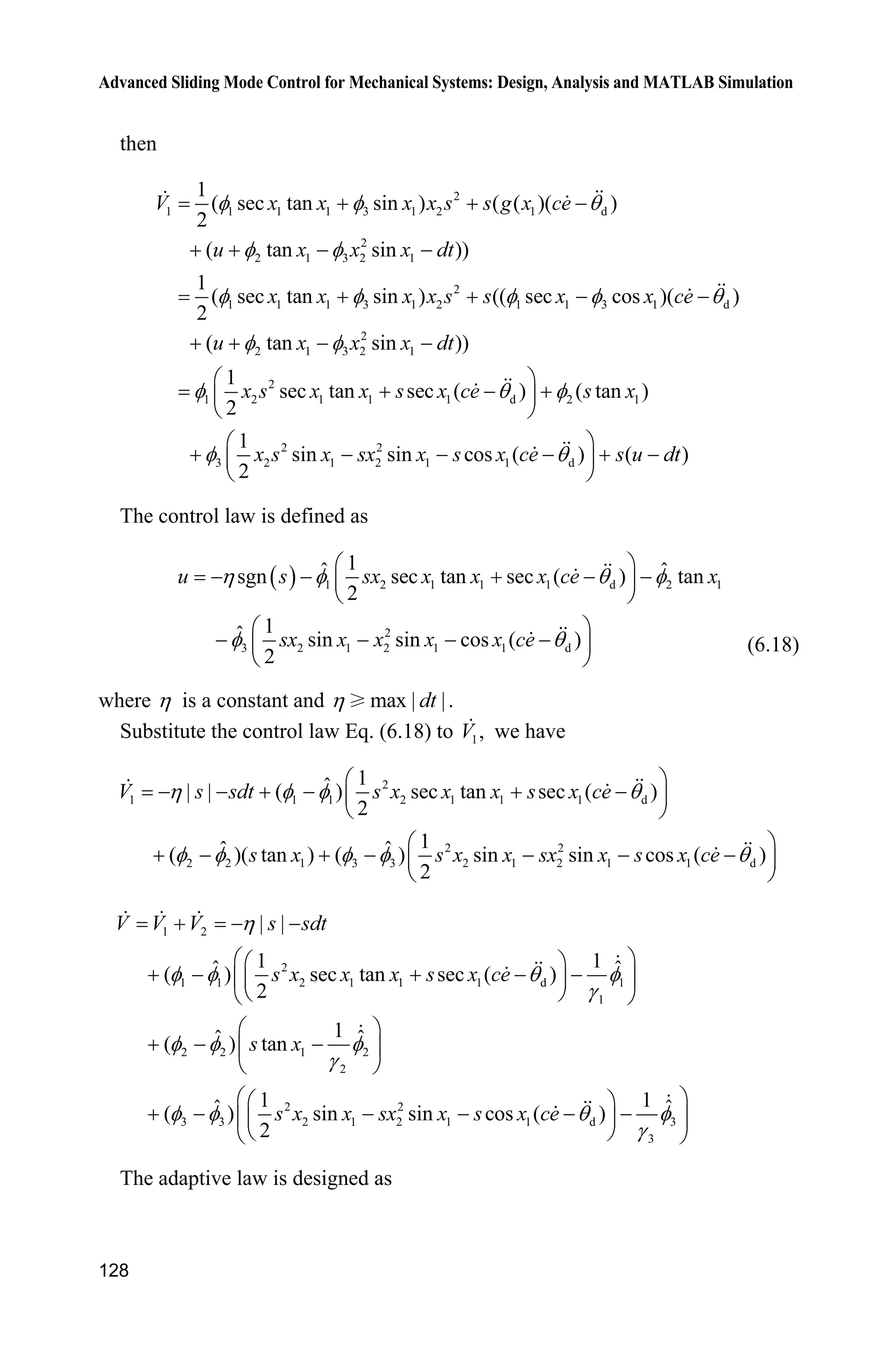
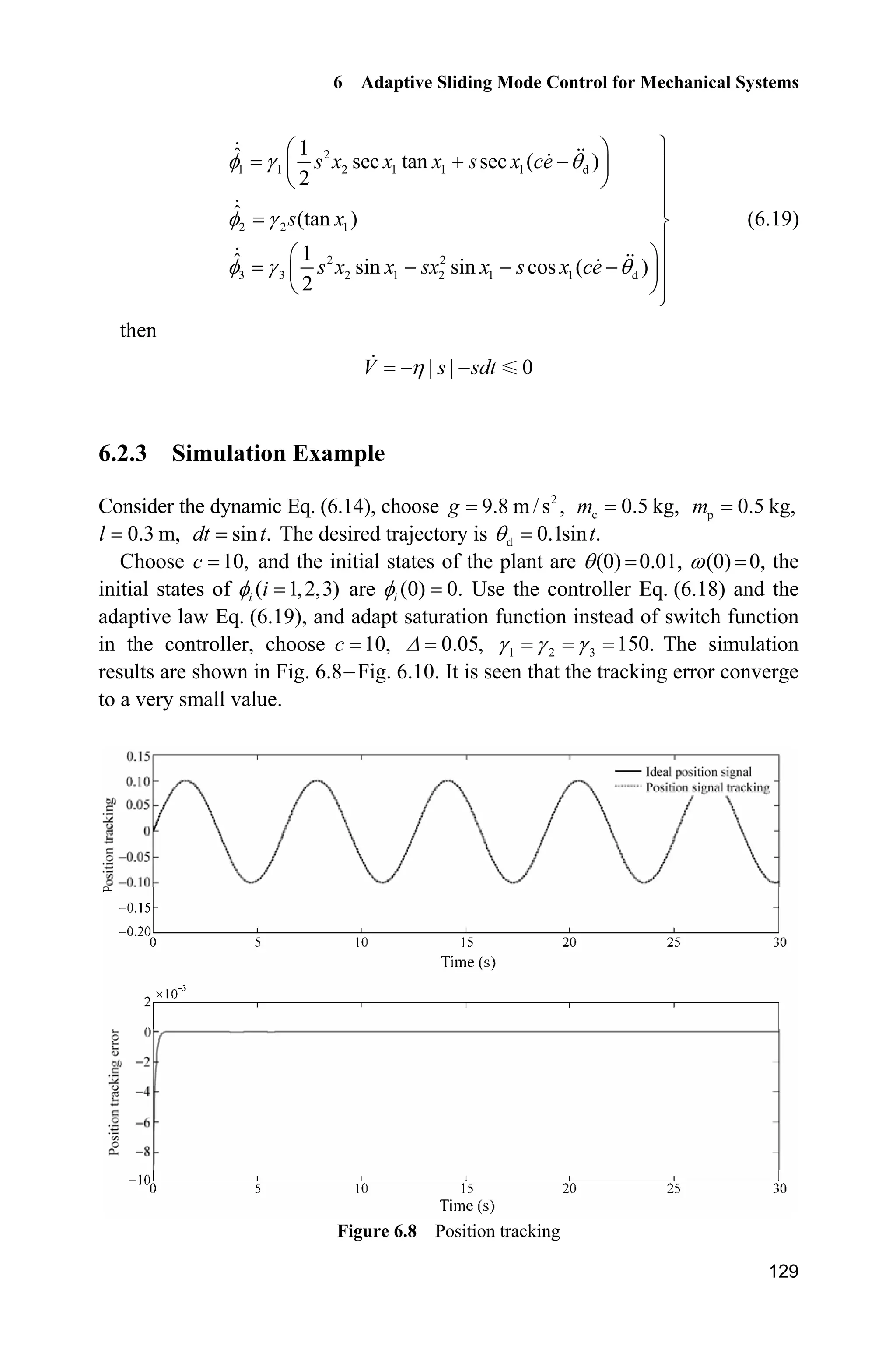
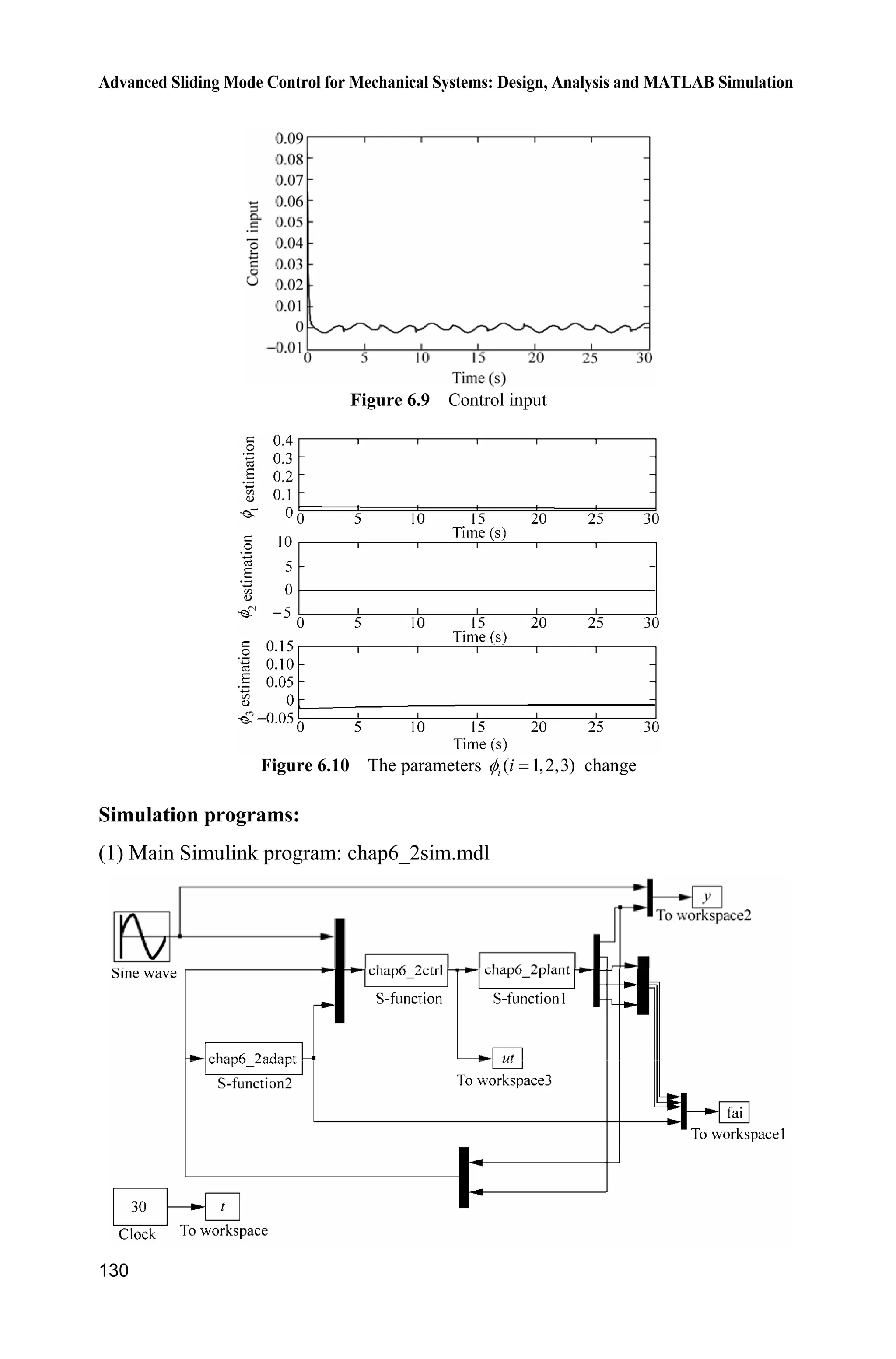
![6 Adaptive Sliding Mode Control for Mechanical Systems
131
(2) Control law program: chap6_2ctrl.m
function [sys,x0,str,ts]=s_function(t,x,u,flag)
switch flag,
case 0,
[sys,x0,str,ts]=mdlInitializeSizes;
case 3,
sys=mdlOutputs(t,x,u);
case {1,2, 4, 9 }
sys = [];
otherwise
error(['Unhandled flag = ',num2str(flag)]);
end
function [sys,x0,str,ts]=mdlInitializeSizes
sizes = simsizes;
sizes.NumContStates = 0;
sizes.NumDiscStates = 0;
sizes.NumOutputs = 1;
sizes.NumInputs = 6;
sizes.DirFeedthrough = 1;
sizes.NumSampleTimes = 1;
sys=simsizes(sizes);
x0=[];
str=[];
ts=[0 0];
function sys=mdlOutputs(t,x,u)
thd=u(1);
dthd=0.1*cos(t);
ddthd=-0.1*sin(t);
x1=u(2);
x2=u(3);
fai1p=u(4);
fai2p=u(5);
fai3p=u(6);
e=x1-thd;
de=x2-dthd;
c=10;
s=c*e+de;
xite=1.0;
delta=0.05;
kk=1/delta;
if abs(s)delta
sats=sign(s);
else
sats=kk*s;](https://image.slidesharecdn.com/advancedslidingmodecontrolformechanicalsystems-130611121131-phpapp01/75/Advanced-sliding-mode-control-for-mechanical-systems-147-2048.jpg)
![Advanced Sliding Mode Control for Mechanical Systems: Design, Analysis and MATLAB Simulation
132
end
delta=0.05;
kk=1/delta;
if abs(s)delta
sats=sign(s);
else
sats=kk*s;
end
%ut=-xite*sign(s)-fai1p*(0.5*s*x2*sec(x1)*tan(x1)+sec(x1)*(c*de-ddthd))
-fai2p*tan(x1)-fai3p*(0.5*s*x2*sin(x1)-x2^2*sin(x1)-cos(x1)*(c*de-ddthd));
ut=-xite*sats-fai1p*(0.5*s*x2*sec(x1)*tan(x1)+sec(x1)*(c*de-ddthd))-fai2p
*tan(x1)-fai3p*(0.5*s*x2*sin(x1)-x2^2*sin(x1)-cos(x1)*(c*de-ddthd));
sys(1)=ut;
(3) Plant S-function: chap6_2plant.m
function [sys,x0,str,ts]=s_function(t,x,u,flag)
switch flag,
case 0,
[sys,x0,str,ts]=mdlInitializeSizes;
case 1,
sys=mdlDerivatives(t,x,u);
case 3,
sys=mdlOutputs(t,x,u);
case {2, 4, 9 }
sys = [];
otherwise
error(['Unhandled flag = ',num2str(flag)]);
end
function [sys,x0,str,ts]=mdlInitializeSizes
sizes = simsizes;
sizes.NumContStates = 2;
sizes.NumDiscStates = 0;
sizes.NumOutputs = 5;
sizes.NumInputs = 1;
sizes.DirFeedthrough = 1;
sizes.NumSampleTimes = 0;
sys=simsizes(sizes);
x0=[0.01;0];
str=[];
ts=[];
function sys=mdlDerivatives(t,x,u)
F=u(1);
mc=0.5;mp=0.5;
l=0.3;
I=0.006;
g=9.8;](https://image.slidesharecdn.com/advancedslidingmodecontrolformechanicalsystems-130611121131-phpapp01/75/Advanced-sliding-mode-control-for-mechanical-systems-148-2048.jpg)
![6 Adaptive Sliding Mode Control for Mechanical Systems
133
fai1=(mc+mp)*(I+mp*l^2)/(mp*l);
fai2=(mc+mp)*g;
fai3=mp*l;
gx1=fai1*sec(x(1))-fai3*cos(x(1));
dt=1.0*sin(t);
sys(1)=x(2);
sys(2)=1/gx1*(u-dt+fai2*tan(x(1))-fai3*x(2)^2*sin(x(1)));
function sys=mdlOutputs(t,x,u)
mc=0.5;mp=0.5;
l=0.3;
I=1/3*mp*l^2;
g=9.8;
fai1=(mc+mp)*(I+mp*l^2)/(mp*l);
fai2=(mc+mp)*g;
fai3=mp*l;
sys(1)=x(1);
sys(2)=x(2);
sys(3)=fai1;
sys(4)=fai2;
sys(5)=fai3;
(4) Adaptive law S-function: chap6_2adapt.m
function [sys,x0,str,ts]=s_function(t,x,u,flag)
switch flag,
case 0,
[sys,x0,str,ts]=mdlInitializeSizes;
case 1,
sys=mdlDerivatives(t,x,u);
case 3,
sys=mdlOutputs(t,x,u);
case {2, 4, 9 }
sys = [];
otherwise
error(['Unhandled flag = ',num2str(flag)]);
end
function [sys,x0,str,ts]=mdlInitializeSizes
sizes = simsizes;
sizes.NumContStates = 3;
sizes.NumDiscStates = 0;
sizes.NumOutputs = 3;
sizes.NumInputs = 2;](https://image.slidesharecdn.com/advancedslidingmodecontrolformechanicalsystems-130611121131-phpapp01/75/Advanced-sliding-mode-control-for-mechanical-systems-149-2048.jpg)
![Advanced Sliding Mode Control for Mechanical Systems: Design, Analysis and MATLAB Simulation
134
sizes.DirFeedthrough = 1;
sizes.NumSampleTimes = 0;
sys=simsizes(sizes);
x0=[0 0 0];
str=[];
ts=[];
function sys=mdlDerivatives(t,x,u)
x1=u(1);
x2=u(2);
thd=0.1*sin(t);
dthd=0.1*cos(t);
ddthd=-0.1*sin(t);
e=x1-thd;
de=x2-dthd;
c=10;
s=c*e+de;
gama1=150;gama2=150;gama3=150;
sys(1)=gama1*(0.5*s^2*x2*sec(x1)*tan(x1)+s*sec(x1)*(c*de-ddthd));
sys(2)=gama2*s*tan(x1);
sys(3)=gama3*(0.5*s^2*x2*sin(x1)-s*x2^2*sin(x1)-s*cos(x1)*(c*de-ddthd));
function sys=mdlOutputs(t,x,u)
sys(1)=x(1); %fai1
sys(2)=x(2); %fai2
sys(3)=x(3); %fai3
(5) Plot program: chap6_2plot.m
close all;
figure(1);
subplot(211);
plot(t,y(:,1),'k',t,y(:,2),'r:','linewidth',2);
xlabel('time(s)');ylabel('Position tracking');
legend('Ideal position signal','Position signal tracking');
subplot(212);
plot(t,y(:,1)-y(:,2),'r','linewidth',2);
xlabel('time(s)');ylabel('Position tracking error');
figure(2);
plot(t,ut(:,1),'r','linewidth',2);
xlabel('time(s)');ylabel('Control input');
figure(3);
subplot(311);](https://image.slidesharecdn.com/advancedslidingmodecontrolformechanicalsystems-130611121131-phpapp01/75/Advanced-sliding-mode-control-for-mechanical-systems-150-2048.jpg)
![6 Adaptive Sliding Mode Control for Mechanical Systems
135
plot(t,fai(:,1),'k',t,fai(:,4),'r','linewidth',2);
xlabel('time(s)');ylabel('fai1 estimation');
subplot(312);
plot(t,fai(:,2),'k',t,fai(:,5),'r','linewidth',2);
xlabel('time(s)');ylabel('fai2 estimation');
subplot(313);
plot(t,fai(:,3),'k',t,fai(:,6),'r','linewidth',2);
xlabel('time(s)');ylabel('fai3 estimation');
References
[1] Xu L, Yao B. Adaptive robust control of mechanical systems with non-linear dynamic friction
compensation, International Journal of control, February 2008, 81(2): 167 176
[2] C.Canudas de Wit, Olsson H, Astrom KJ and Lischinsky P. A new model for control of
systems with friction, IEEE Transaction on Automatic Control, 1995, 40: 419 425
[3] Tan Y and Kanellakopoulos I. Adaptive non-linear friction compensation with parametric
uncertainties. Proc. of the American Control Conference, San Diego, 1999, 2511 2515
[4] Ebrahim A, Murphy GV. Adaptive backstepping controller design of an inverted pendulum,
Proceedings of the Thirty-Seventh Southeastern Symposium on System Theory, 2005,
172 174
[5] Slotine JE, Li W. Applied Nonlinear Control. Prentice Hall, 1991](https://image.slidesharecdn.com/advancedslidingmodecontrolformechanicalsystems-130611121131-phpapp01/75/Advanced-sliding-mode-control-for-mechanical-systems-151-2048.jpg)
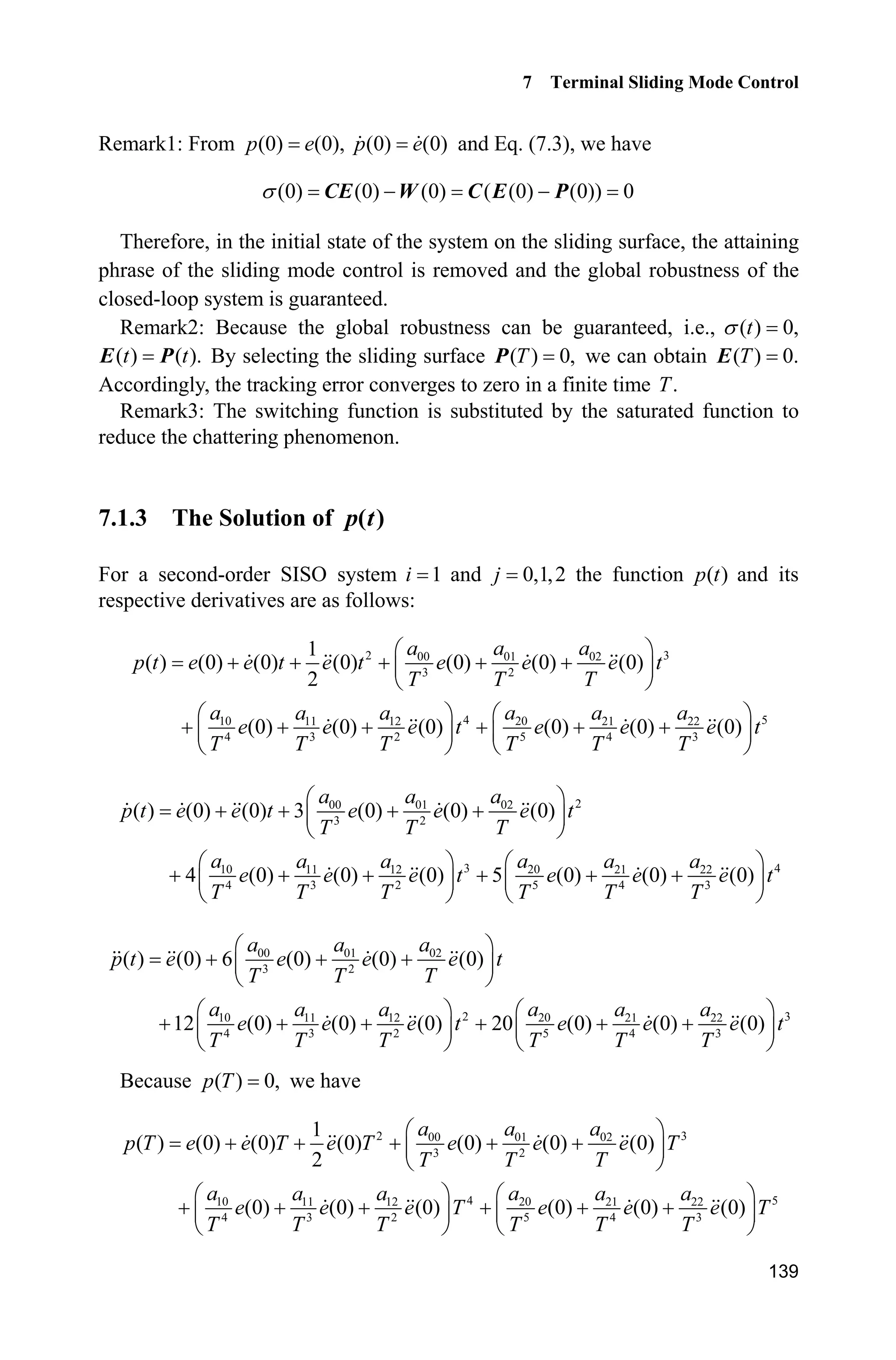
![Advanced Sliding Mode Control for Mechanical Systems: Design, Analysis and MATLAB Simulation
138
7.1.2 Design of Terminal Sliding Mode Controller
In this section, we introduced a terminal sliding mode controller[1]
proposed by
Zhuang et al.
7.1.2.1 Design of Switch Plane
In order to make the states converge to the desired trajectories in a finite time the
sliding variable proposed in[1]
as:
( )V C E P (7.3)
where [ 1],cC c0 must be Hurwitz, T
[ ] ,e eE T
[ ( ) ( )] ,p t p tP e
1 1dx x is the tracking error, and 1dx is the desired trajectory.
The design rule of ( )p t is: for 0,T ! ( )p t has the upper boundless on [0, ].T
In order to guarantee (0) 0,V let (0) (0),E P i.e. (0) (0),p e (0) (0);p e at
the same time, we make ( ) 0,p T ( ) 0p T and ( ) 0.p T
According to the above condition, Zhuang et al. designed ( )p t as
2 2 2
( ) ( ) 3
3
0 0 0
1
(0) (0) , 0
( ) !
0,
§ ·
˜° ¨ ¸
® © ¹
°
!¯
¦ ¦ ¦ jlk k l j
i ij l
k j l
a
e t e t t T
p t k T
t T
(7.4)
where jla is constant and can be obtained by solving the equations[1]
.
7.1.2.2 Design of Terminal Sliding Mode Controller
From Eq. (7.3), we get
T T
[ ] [ , ] ( ) ( )e,e p p c e p e pV CE CP C C
i.e.
d( ) ( ) ( ) ( )c e p f x g x u d t x pV
Select the Lyapunov function as:
21
2
V V (7.5)
The controller can be designed as:
d
1
( ) ( ( ) ( ) sgn( ))
( )
t f x x p c e p
g x
K V u (7.6)
where .DK Therefore, we have
( sgn( ) ( )) | | ( ) 0V d t d tVV V K V K V V](https://image.slidesharecdn.com/advancedslidingmodecontrolformechanicalsystems-130611121131-phpapp01/75/Advanced-sliding-mode-control-for-mechanical-systems-153-2048.jpg)
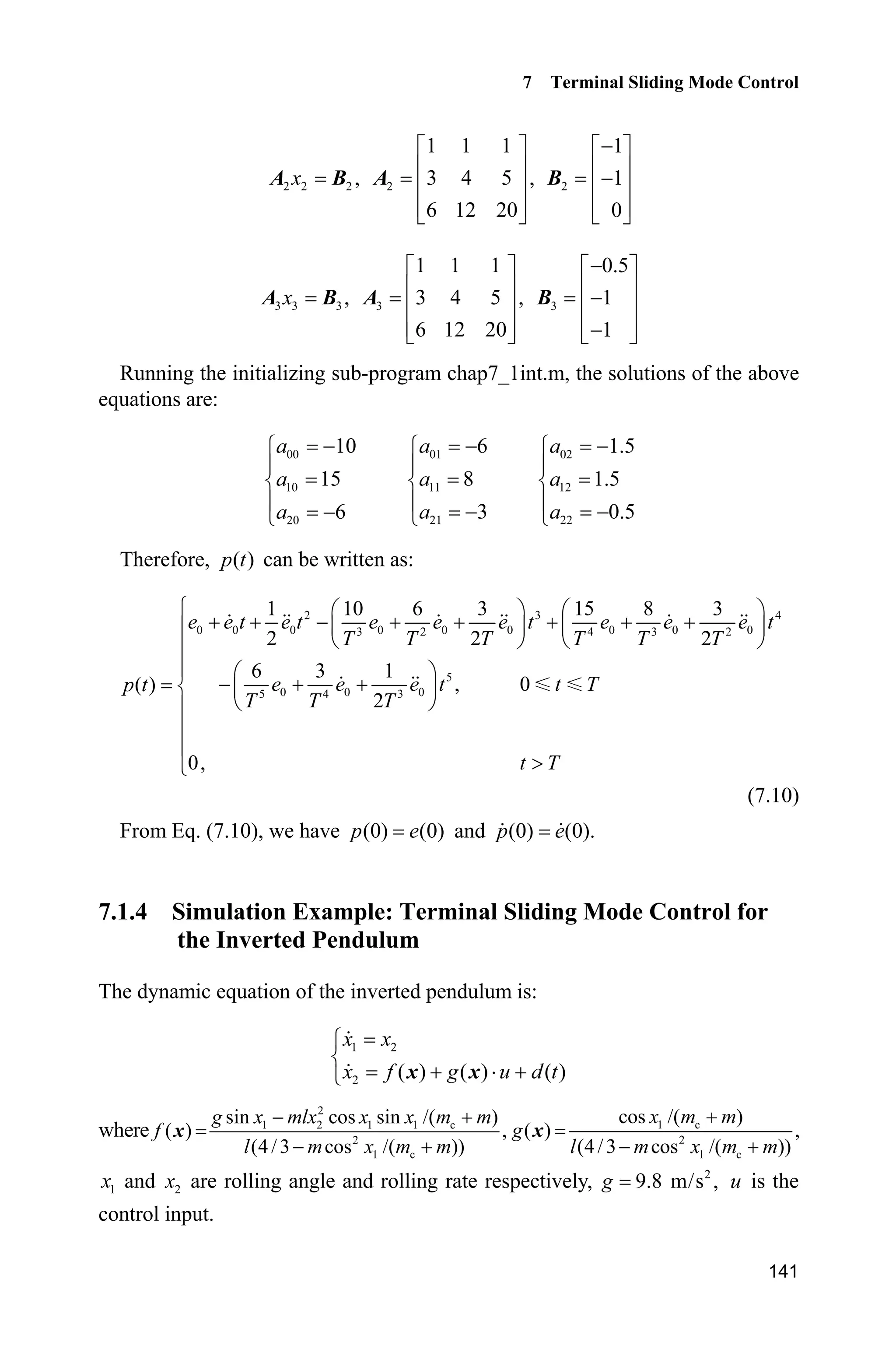
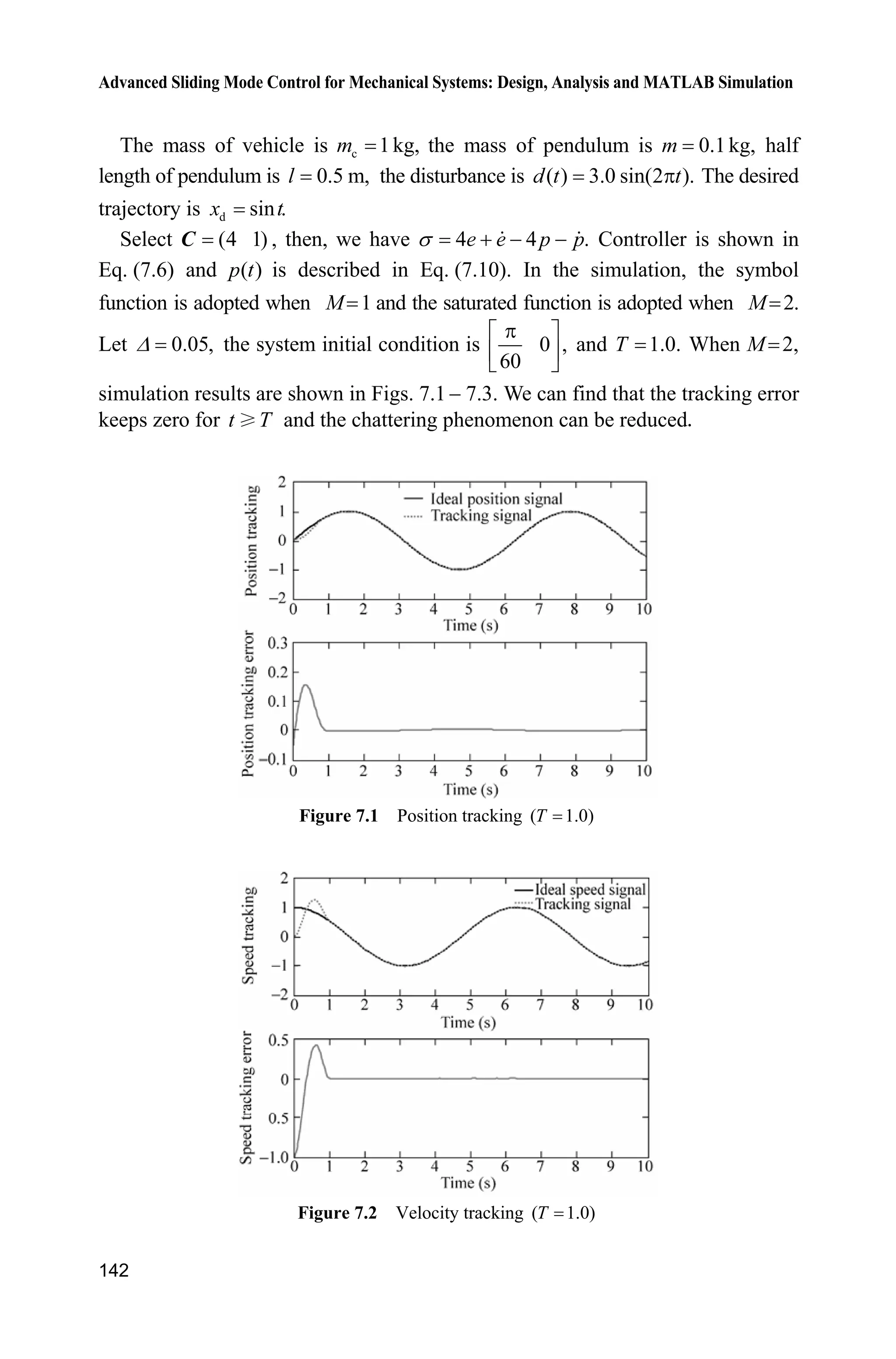
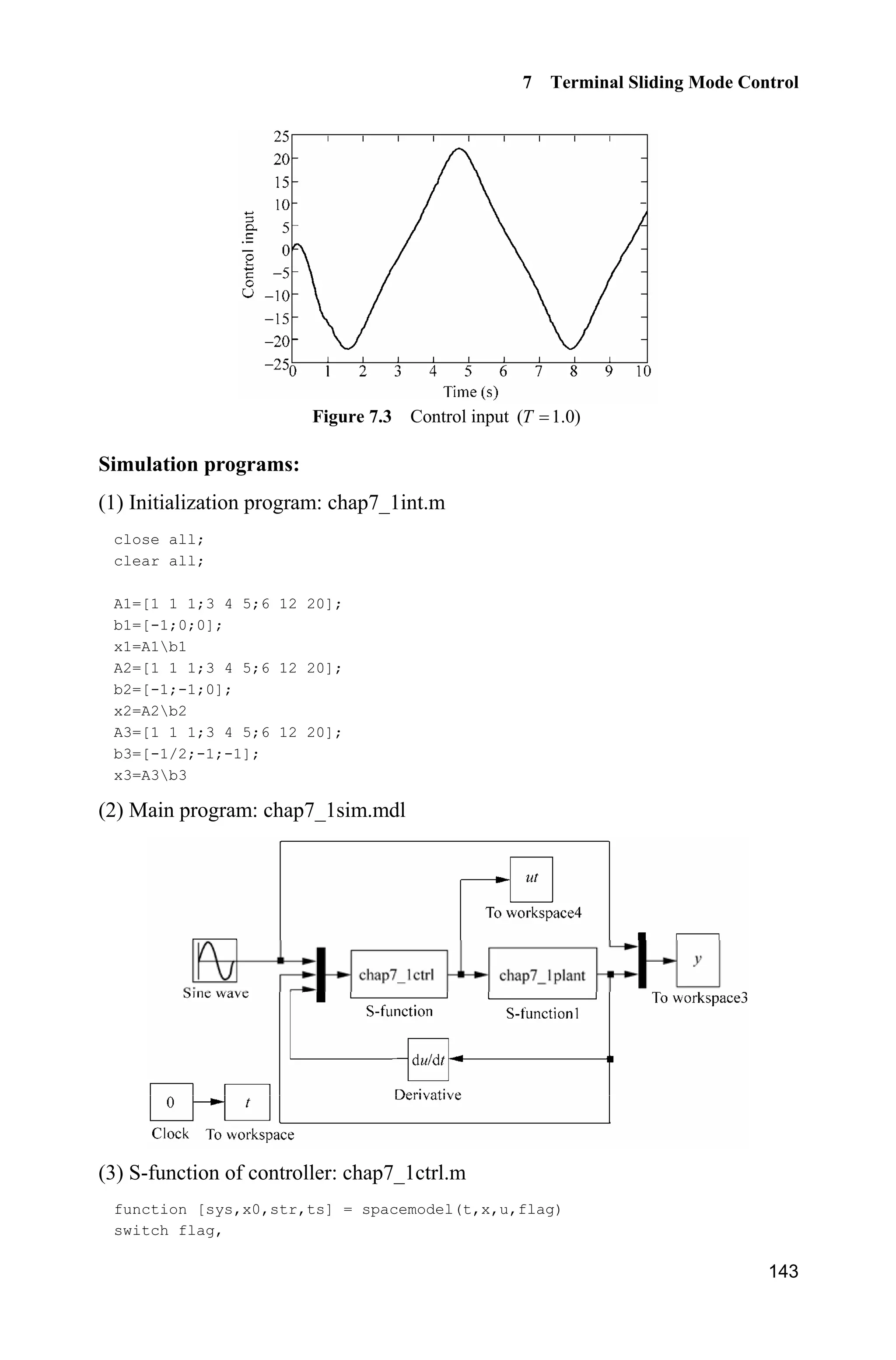
![7 Terminal Sliding Mode Control
143
Figure 7.3 Control input ( 1.0)T
Simulation programs:
(1) Initialization program: chap7_1int.m
close all;
clear all;
A1=[1 1 1;3 4 5;6 12 20];
b1=[-1;0;0];
x1=A1b1
A2=[1 1 1;3 4 5;6 12 20];
b2=[-1;-1;0];
x2=A2b2
A3=[1 1 1;3 4 5;6 12 20];
b3=[-1/2;-1;-1];
x3=A3b3
(2) Main program: chap7_1sim.mdl
(3) S-function of controller: chap7_1ctrl.m
function [sys,x0,str,ts] = spacemodel(t,x,u,flag)
switch flag,](https://image.slidesharecdn.com/advancedslidingmodecontrolformechanicalsystems-130611121131-phpapp01/75/Advanced-sliding-mode-control-for-mechanical-systems-160-2048.jpg)
![Advanced Sliding Mode Control for Mechanical Systems: Design, Analysis and MATLAB Simulation
144
case 0,
[sys,x0,str,ts]=mdlInitializeSizes;
case 3,
sys=mdlOutputs(t,x,u);
case {2,4,9}
sys=[];
otherwise
error(['Unhandled flag = ',num2str(flag)]);
end
function [sys,x0,str,ts]=mdlInitializeSizes
sizes = simsizes;
sizes.NumContStates = 0;
sizes.NumDiscStates = 0;
sizes.NumOutputs = 1;
sizes.NumInputs = 5;
sizes.DirFeedthrough = 1;
sizes.NumSampleTimes = 1;
sys = simsizes(sizes);
x0 = [];
str = [];
ts = [0 0];
function sys=mdlOutputs(t,x,u)
persistent e0 de0 dde0
T=1.0;
xd=u(1);dxd=cos(t);ddxd=-sin(t);
x1=u(2);x2=u(3);
dx1=u(4);dx2=u(5);
if t==0
e0=x1;
de0=x2-1;
dde0=dx2;
end
e=x1-xd;
de=x2-dxd;
if t=T
A0=-10/T^3*e0-6/T^2*de0-1.5/T*dde0;
A1=15/T^4*e0+8/T^3*de0+1.5/T^2*dde0;
A2=-6/T^5*e0-3/T^4*de0-0.5/T^3*dde0;
p=e0+de0*t+1/2*dde0*t^2+A0*t^3+A1*t^4+A2*t^5;
dp=de0+dde0*t+A0*3*t^2+A1*4*t^3+A2*5*t^4;
ddp=dde0+A0*3*2*t+A1*4*3*t^2+A2*5*4*t^3;
else
p=0;dp=0;ddp=0;
end
c=15;
rou=(c*e+de)-(c*p+dp);
%%%%%%%%%%%%%%%%%%%%%%%%%%%%%%%%%%%%%%
g=9.8;mc=1.0;m=0.1;l=0.5;
S=l*(4/3-m*(cos(x1))^2/(mc+m));](https://image.slidesharecdn.com/advancedslidingmodecontrolformechanicalsystems-130611121131-phpapp01/75/Advanced-sliding-mode-control-for-mechanical-systems-161-2048.jpg)
![7 Terminal Sliding Mode Control
145
fx=g*sin(x1)-m*l*x2^2*cos(x1)*sin(x1)/(mc+m);
fx=fx/S;
gx=cos(x1)/(mc+m);
gx=gx/S;
%%%%%%%%%%%%%%%%%%%%%%%%%%%%%%%%%%%%%%
delta=0.05;
if abs(rou)delta
sat=sign(rou);
else
sat=1/delta*rou;
end
xite=3.1;
M=2;
if M==1
ut=-1/gx*(fx-ddxd-ddp+c*(de-dp)+xite*sign(rou));
elseif M==2
ut=-1/gx*(fx-ddxd-ddp+c*(de-dp)+xite*sat);
end
sys(1)=ut;
(4) S-function of the plant: chap7_1plant.m
function [sys,x0,str,ts]=s_function(t,x,u,flag)
switch flag,
case 0,
[sys,x0,str,ts]=mdlInitializeSizes;
case 1,
sys=mdlDerivatives(t,x,u);
case 3,
sys=mdlOutputs(t,x,u);
case {2, 4, 9 }
sys = [];
otherwise
error(['Unhandled flag = ',num2str(flag)]);
end
function [sys,x0,str,ts]=mdlInitializeSizes
sizes = simsizes;
sizes.NumContStates = 2;
sizes.NumDiscStates = 0;
sizes.NumOutputs = 2;
sizes.NumInputs = 1;
sizes.DirFeedthrough = 0;
sizes.NumSampleTimes = 0;
sys=simsizes(sizes);
x0=[pi/60 0];
str=[];
ts=[];
function sys=mdlDerivatives(t,x,u)
g=9.8;mc=1.0;m=0.1;l=0.5;
S=l*(4/3-m*(cos(x(1)))^2/(mc+m));
fx=g*sin(x(1))-m*l*x(2)^2*cos(x(1))*sin(x(1))/(mc+m);
fx=fx/S;
gx=cos(x(1))/(mc+m);](https://image.slidesharecdn.com/advancedslidingmodecontrolformechanicalsystems-130611121131-phpapp01/75/Advanced-sliding-mode-control-for-mechanical-systems-162-2048.jpg)
![Advanced Sliding Mode Control for Mechanical Systems: Design, Analysis and MATLAB Simulation
146
gx=gx/S;
%%%%%%%%%
dt=3*sin(t);
%%%%%%%%%
sys(1)=x(2);
sys(2)=fx+gx*u+dt;
function sys=mdlOutputs(t,x,u)
sys(1)=x(1);
sys(2)=x(2);
(5) Plot program: chap7_1plot.m
close all;
figure(1);
subplot(211);
plot(t,y(:,1),'k',t,y(:,2),'r:','linewidth',2);
xlabel('time(s)');ylabel('Position tracking');
legend('Ideal position signal','tracking signal');
subplot(212);
plot(t,y(:,2)-y(:,1),'r','linewidth',2);
xlabel('time(s)');ylabel('Position tracking error');
figure(2);
subplot(211);
plot(t,cos(t),'k',t,y(:,3),'r:','linewidth',2);
xlabel('time(s)');ylabel('Speed tracking');
legend('Ideal speed signal','tracking signal');
subplot(212);
plot(t,y(:,3)-cos(t),'r','linewidth',2);
xlabel('time(s)');ylabel('Speed tracking error');
figure(3);
plot(t,ut,'r','linewidth',2);
xlabel('time(s)');ylabel('control input');
7.2 Nonsingular Terminal Sliding Mode Control
7.2.1 System Description
Consider the second-order uncertain nonlinear system as under:
1 2
2 ( ) ( ) ( , )
x x
x f g u d t
½
¾
¿x x x
(7.11)
where T
1 2 1 2[ ] , andx x x xx are system states, ( ) 0,g zx ( , )d tx is the uncertainty
or disturbance, | ( , ) |d t Lx .](https://image.slidesharecdn.com/advancedslidingmodecontrolformechanicalsystems-130611121131-phpapp01/75/Advanced-sliding-mode-control-for-mechanical-systems-163-2048.jpg)
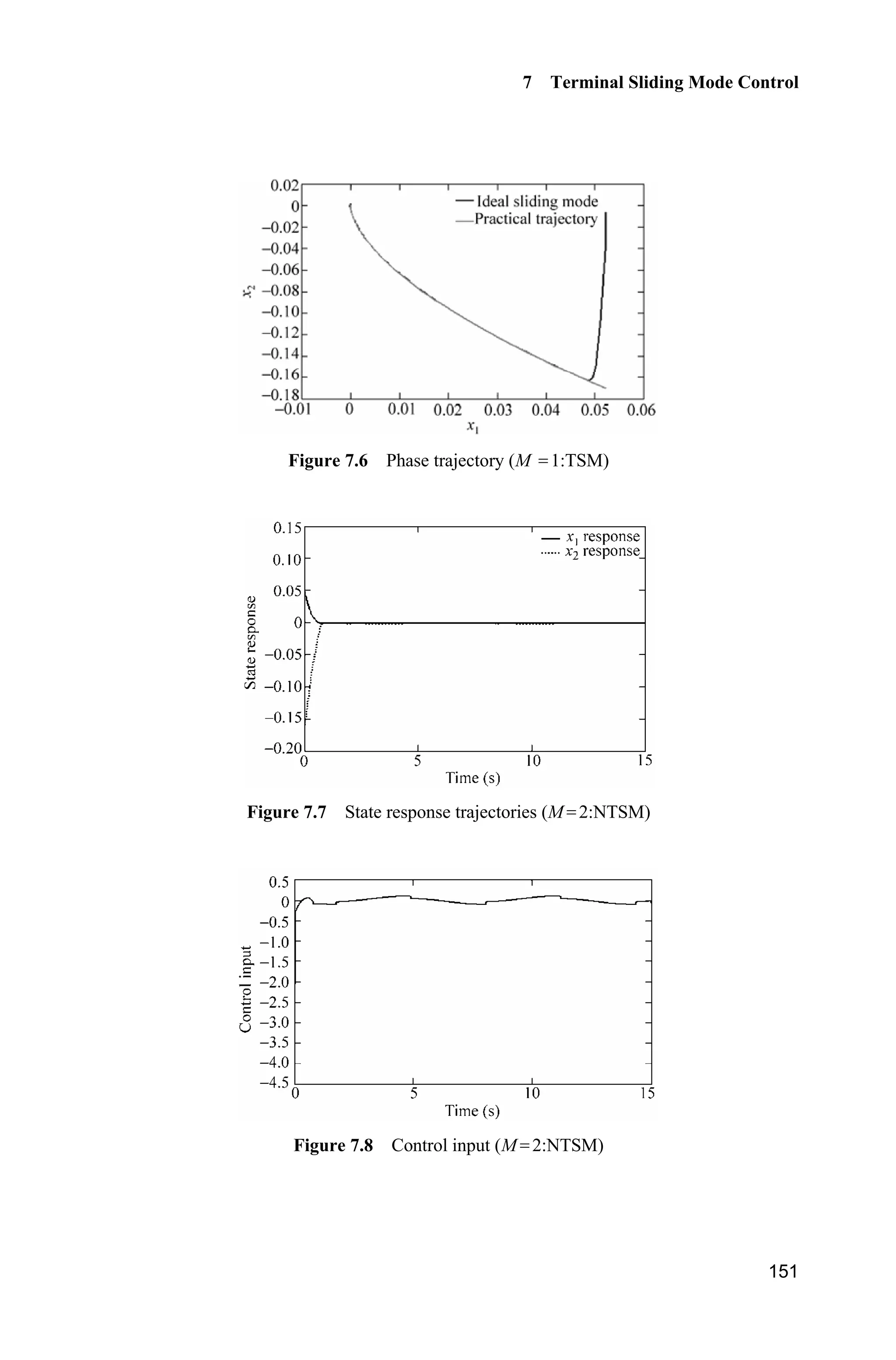
![Advanced Sliding Mode Control for Mechanical Systems: Design, Analysis and MATLAB Simulation
148
At the same time, when 0,s
(0)
,r
s
t
K
i.e.,
| (0) |
r
s
t
K
(7.14)
Suppose the attaining time is st from 1( ) 0rx t z to 1( ) 0.s rx t t In this phase,
0,s i.e.,
/
2 1 0q p
x xE
1 1
q
p
x xE
Integrating the above differential equation, we have
1
0
1 1( )
d d
r s
r r
q
t t
p
x t t
x x tE
³ ³
1
1 ( )
q
p
r s
p
x t t
p q
E
1
1| ( ) |
( )
q
p
s r
p
t x t
p qE
(7.15)
7.2.3 Nonsingular Terminal Sliding Mode Control
A nonsingular terminal sliding mode control method is proposed by Feng et al.[2]
to deal with the singular problem of normal terminal sliding mode control.
The nonsingular sliding variable is designed by Feng et al. as:
/
1 2
1 p q
s x x
E
(7.16)
where 0, , ( )p q p qE ! ! are positive odd numbers[2]
.
The nonsingular sliding mode controller is designed by Feng et al. as:
1 2 /
2( ) ( ) ( )sgn( )p qq
u g f x L s
p
E K § ·
¨ ¸
© ¹
x x (7.17)
where 1 / 2,p q 0.K !
Analysis of stability](https://image.slidesharecdn.com/advancedslidingmodecontrolformechanicalsystems-130611121131-phpapp01/75/Advanced-sliding-mode-control-for-mechanical-systems-165-2048.jpg)
![Advanced Sliding Mode Control for Mechanical Systems: Design, Analysis and MATLAB Simulation
152
Figure 7.9 Phase trajectories (M 2:NTSM)
Simulation programs:
(1) Main program: chap7_2sim.mdl
(2) S-function of control input: chap7_2ctrl.m
function [sys,x0,str,ts]=s_function(t,x,u,flag)
switch flag,
case 0,
[sys,x0,str,ts]=mdlInitializeSizes;
case 3,
sys=mdlOutputs(t,x,u);
case {2, 4, 9 }
sys = [];
otherwise
error(['Unhandled flag = ',num2str(flag)]);
end
function [sys,x0,str,ts]=mdlInitializeSizes
sizes = simsizes;
sizes.NumContStates = 0;
sizes.NumDiscStates = 0;
sizes.NumOutputs = 1;
sizes.NumInputs = 2;
sizes.DirFeedthrough = 1;](https://image.slidesharecdn.com/advancedslidingmodecontrolformechanicalsystems-130611121131-phpapp01/75/Advanced-sliding-mode-control-for-mechanical-systems-169-2048.jpg)
![7 Terminal Sliding Mode Control
153
sizes.NumSampleTimes = 0;
sys=simsizes(sizes);
x0=[];
str=[];
ts=[];
function sys=mdlOutputs(t,x,u)
x1=u(1);x2=u(2);
g=9.8;mc=1.0;m=0.1;l=0.5;
S=l*(4/3-m*(cos(x1))^2/(mc+m));
fx=g*sin(x1)-m*l*x2^2*cos(x1)*sin(x1)/(mc+m);
fx=fx/S;
gx=cos(x1)/(mc+m);
gx=gx/S;
L=5;
beta=1.0;
xite=0.3;
q=3;p=5;
M=1;
if M==1 %TSM
T1=abs(x1)^(q/p)*sign(x1);
T2=abs(x1)^(q/p-1)*sign(x1);
s=x2+beta*T1;
delta=0.015;
kk=1/delta;
if abs(s)delta
sats=sign(s);
else
sats=kk*s;
end
% ut=-inv(gx)*(fx+beta*q/p*T2*x2+(L+xite)*sign(s));
ut=-inv(gx)*(fx+beta*q/p*T2*x2+(L+xite)*sats); %With saturation
elseif M==2 %NTSM
T1=abs(x2)^(p/q)*sign(x2);
T2=abs(x2)^(2-p/q)*sign(x2);
s=x1+1/beta*T1;
delta=0.015;
kk=1/delta;
if abs(s)delta
sats=sign(s);
else
sats=kk*s;
end
% ut=-inv(gx)*(fx+beta*q/p*T2+(L+xite)*sign(s));
ut=-inv(gx)*(fx+beta*q/p*T2+(L+xite)*sats); %With saturation](https://image.slidesharecdn.com/advancedslidingmodecontrolformechanicalsystems-130611121131-phpapp01/75/Advanced-sliding-mode-control-for-mechanical-systems-170-2048.jpg)
![Advanced Sliding Mode Control for Mechanical Systems: Design, Analysis and MATLAB Simulation
154
end
sys(1)=ut;
(3) S-function of the plant: chap7_2plant.m
function [sys,x0,str,ts]=s_function(t,x,u,flag)
switch flag,
case 0,
[sys,x0,str,ts]=mdlInitializeSizes;
case 1,
sys=mdlDerivatives(t,x,u);
case 3,
sys=mdlOutputs(t,x,u);
case {2, 4, 9 }
sys = [];
otherwise
error(['Unhandled flag = ',num2str(flag)]);
end
function [sys,x0,str,ts]=mdlInitializeSizes
sizes = simsizes;
sizes.NumContStates = 2;
sizes.NumDiscStates = 0;
sizes.NumOutputs = 2;
sizes.NumInputs = 1;
sizes.DirFeedthrough = 0;
sizes.NumSampleTimes = 0;
sys=simsizes(sizes);
x0=[pi/60 0];
str=[];
ts=[];
function sys=mdlDerivatives(t,x,u)
g=9.8;mc=1.0;m=0.1;l=0.5;
S=l*(4/3-m*(cos(x(1)))^2/(mc+m));
fx=g*sin(x(1))-m*l*x(2)^2*cos(x(1))*sin(x(1))/(mc+m);
fx=fx/S;
gx=cos(x(1))/(mc+m);
gx=gx/S;
%%%%%%%%%
dt=0.1*sin(t);
%%%%%%%%%
sys(1)=x(2);
sys(2)=fx+gx*u+dt;
function sys=mdlOutputs(t,x,u)
sys(1)=x(1);
sys(2)=x(2);
(4) Plot program: chap7_2plot.m
close all;
figure(1);](https://image.slidesharecdn.com/advancedslidingmodecontrolformechanicalsystems-130611121131-phpapp01/75/Advanced-sliding-mode-control-for-mechanical-systems-171-2048.jpg)
![7 Terminal Sliding Mode Control
155
plot(t,x(:,1),'k',t,x(:,2),'k:','linewidth',2);
xlabel('time(s)');ylabel('State response');
legend('x1 response','x2 response');
figure(2);
plot(t,ut(:,1),'r','linewidth',2);
xlabel('time(s)');ylabel('Control input');
figure(3);
M=1;
q=3;p=5;
if M==1 %TSM
plot(x(:,1),x(:,2),'k',x(:,1),-(abs(x(:,1))).^(q/p).*sign(x(:,1)),'r','lin
ewidth',2);
legend('ideal sliding mode','practical trajectory');
elseif M==2 %NTSM
plot(x(:,1),x(:,2),'k',x(:,1),(abs(-x(:,1))).^(q/p).*sign(-x(:,1)),'r','li
newidth',2);
legend('ideal sliding mode','practical trajectory');
end
xlabel('x1');ylabel('x2');
7.3 Fast Terminal Sliding Mode Control
Fast Terminal sliding mode control can make the system states converge to zero in
a finite time. Asymptotical convergence of states under the normal sliding mode
is overcome. The convergent characteristic of fast terminal sliding mode control is
superior to that of the normal sliding mode control. Moreover, there is no switch
function in terminal sliding mode control, therefore, the chattering phenomenon
is evitable.
7.3.1 Design of Fast Terminal Sliding Mode Controller
7.3.1.1 Traditional Terminal Sliding Surface
A kind of fast terminal sliding surface was proposed by park et al. as follows:
/
0q p
s x xE (7.18)
where xR is the state, 0, , ( )p q p qE ! ! are positive odd numbers[3]
.
From Eq. (7.18), we have
/d
d
q px
x
t
E](https://image.slidesharecdn.com/advancedslidingmodecontrolformechanicalsystems-130611121131-phpapp01/75/Advanced-sliding-mode-control-for-mechanical-systems-172-2048.jpg)
![Advanced Sliding Mode Control for Mechanical Systems: Design, Analysis and MATLAB Simulation
156
i.e.,
/1
d dq p
t x x
E
Therefore,
0
0
/
0
1
d d
t
q p
x
t x x
E
³ ³
The time interval that the initial state (0) 0x z takes to attain equilibrium 0x
along the sliding surface Eq. (7.18) is:
( ) /
| (0) |
( )
p q p
s
p
t x
p qE
(7.19)
The equilibrium 0x is called as the terminal attractor. The convergent velocity
increases as the nonlinear part /q p
xE is introduced. However, the convergent
time of the terminal sliding mode control may not be optimal. This is because the
convergent velocity of nonlinear sliding surface Eq. (7.19) is slower than that of
the linear one ( )p q when the state approaches equilibrium. Therefore, a new
global fast terminal sliding surface was presented in[3]
.
7.3.1.2 Global Fast Terminal Sliding Surface
Considering the linear and the terminal sliding surfaces a new global fast terminal
sliding surface proposed by Park et al. as follows:
/
0q p
s x x xD E (7.20)
where xR is state, , 0,D E ! and ( )p q p q! are positive odd numbers[3]
.
The time interval that the initial state (0) 0x z attains at 0x is:
( ) /
(0)
ln
( )
p q p
s
p x
t
p q
D E
D E
(7.21)
By designing , , ,p qD E we can make the system state attain equilibrium in a
finite time .st From Eq. (7.20), we have
/q p
x x xD E (7.22)
When the state x is far away from the origin, then, the convergent time is
decided by the fast terminal attractor /
;q p
x xE when the state x approaches
the origin 0,x then, the convergent time is decided by the equation .x xD
Exponentially, x converges to zero. Therefore, the terminal attractor is introduced
in the sliding surface Eq. (7.20) and makes the state converge to zero in a finite
time. Moreover, the speed of the linear sliding surface is guaranteed. Accordingly,](https://image.slidesharecdn.com/advancedslidingmodecontrolformechanicalsystems-130611121131-phpapp01/75/Advanced-sliding-mode-control-for-mechanical-systems-173-2048.jpg)
![7 Terminal Sliding Mode Control
157
the state can converge to equilibrium speedily and precisely. We call the sliding
surface Eq. (7.20) as the global fast sliding surface.
7.3.2 Design of Global Fast Sliding Mode Controller
Consider a SISO second-order nonlinear system as follows:
1 2
2 ( ) ( ) ( )
x x
x f g u d t
½
¾
¿x x
(7.23)
where 1 2 1[ ],x x xx and 2x are system states, ( ), ( )f gx x are smooth functions,
( ) 0,g zx ( )d t denotes the uncertainties and | ( ) |d t L denotes the disturbances.
The fast sliding surface is selected as[3]
:
0 0
1 0 0 0 0 0
q p
s s s sD E (7.24)
where 0 0, 0,D E ! and 0 0 0 0, ( )q p q p are positive odd numbers, 0 1.s x
The global fast sliding mode controller is designed as:
0 0/ /
0 0 0 0 1 1
1 d
( ) ( )
( ) d
q p q p
u t f s s s s
g t
D E I J
§ ·
¨ ¸
© ¹
x
x
(7.25)
where 0.J !
The Lyapunov function is selected as
2
1
1
2
V s
Because
0 0 0 0/ /
1 0 0 0 0 0 0 0 0 0
d d
( ) ( ) ( )
d d
q p q p
s s s s f g u d t s s
t t
D E D E x x
Equation (7.25) is introduced into the above equation, then, we have:
1 1 1 ( )q p
s s s d tI J
Therefore,
2 ( ) /
1 1 1 1 1 ( )q p p
V s s s s s d tI J
(7.26)
We know that ( )p q is an even number because ( ) /
1 1 ( ) 0q p p
s s d tJ
satisfied, i.e., /
1
1
| ( ) |q p
d t
s
J or /
1
1
,q p
L
s
J therefore, we have 0.V](https://image.slidesharecdn.com/advancedslidingmodecontrolformechanicalsystems-130611121131-phpapp01/75/Advanced-sliding-mode-control-for-mechanical-systems-174-2048.jpg)
![7 Terminal Sliding Mode Control
159
Figure 7.10 Position tracking
Figure 7.11 Control input
Simulation programs:
(1) Simulink main program: chap7_3sim.mdl
(2) S-function of controller: chap7_3ctrl.m
function [sys,x0,str,ts]=s_function(t,x,u,flag)
switch flag,
case 0,](https://image.slidesharecdn.com/advancedslidingmodecontrolformechanicalsystems-130611121131-phpapp01/75/Advanced-sliding-mode-control-for-mechanical-systems-176-2048.jpg)
![Advanced Sliding Mode Control for Mechanical Systems: Design, Analysis and MATLAB Simulation
160
[sys,x0,str,ts]=mdlInitializeSizes;
case 3,
sys=mdlOutputs(t,x,u);
case {2, 4, 9 }
sys = [];
otherwise
error(['Unhandled flag = ',num2str(flag)]);
end
function [sys,x0,str,ts]=mdlInitializeSizes
sizes = simsizes;
sizes.NumContStates = 0;
sizes.NumDiscStates = 0;
sizes.NumOutputs = 1;
sizes.NumInputs = 2;
sizes.DirFeedthrough = 1;
sizes.NumSampleTimes = 0;
sys=simsizes(sizes);
x0=[];
str=[];
ts=[];
function sys=mdlOutputs(t,x,u)
x1=u(1);x2=u(2);
g=9.8;mc=1.0;m=0.1;l=0.5;
S=l*(4/3-m*(cos(x1))^2/(mc+m));
fx=g*sin(x1)-m*l*x2^2*cos(x1)*sin(x1)/(mc+m);
fx=fx/S;
gx=cos(x1)/(mc+m);
gx=gx/S;
L=5;
beta=1.0;
xite=0.3;
q=3;p=5;
M=1;
if M==1 %TSM
T1=abs(x1)^(q/p)*sign(x1);
T2=abs(x1)^(q/p-1)*sign(x1);
s=x2+beta*T1;
delta=0.015;
kk=1/delta;
if abs(s)delta
sats=sign(s);
else
sats=kk*s;
end
% ut=-inv(gx)*(fx+beta*q/p*T2*x2+(L+xite)*sign(s));](https://image.slidesharecdn.com/advancedslidingmodecontrolformechanicalsystems-130611121131-phpapp01/75/Advanced-sliding-mode-control-for-mechanical-systems-177-2048.jpg)
![7 Terminal Sliding Mode Control
161
ut=-inv(gx)*(fx+beta*q/p*T2*x2+(L+xite)*sats); %With saturation
elseif M==2 %NTSM
T1=abs(x2)^(p/q)*sign(x2);
T2=abs(x2)^(2-p/q)*sign(x2);
s=x1+1/beta*T1;
delta=0.015;
kk=1/delta;
if abs(s)delta
sats=sign(s);
else
sats=kk*s;
end
% ut=-inv(gx)*(fx+beta*q/p*T2+(L+xite)*sign(s));
ut=-inv(gx)*(fx+beta*q/p*T2+(L+xite)*sats); %With saturation
end
sys(1)=ut;
(3) S-function of the plant: chap7_3plant.m
function [sys,x0,str,ts]=s_function(t,x,u,flag)
switch flag,
case 0,
[sys,x0,str,ts]=mdlInitializeSizes;
case 1,
sys=mdlDerivatives(t,x,u);
case 3,
sys=mdlOutputs(t,x,u);
case {2, 4, 9 }
sys = [];
otherwise
error(['Unhandled flag = ',num2str(flag)]);
end
function [sys,x0,str,ts]=mdlInitializeSizes
sizes = simsizes;
sizes.NumContStates = 2;
sizes.NumDiscStates = 0;
sizes.NumOutputs = 2;
sizes.NumInputs = 1;
sizes.DirFeedthrough = 0;
sizes.NumSampleTimes = 0;
sys=simsizes(sizes);
x0=[pi/60 0];
str=[];
ts=[];
function sys=mdlDerivatives(t,x,u)
g=9.8;mc=1.0;m=0.1;l=0.5;
S=l*(4/3-m*(cos(x(1)))^2/(mc+m));
fx=g*sin(x(1))-m*l*x(2)^2*cos(x(1))*sin(x(1))/(mc+m);
fx=fx/S;
gx=cos(x(1))/(mc+m);](https://image.slidesharecdn.com/advancedslidingmodecontrolformechanicalsystems-130611121131-phpapp01/75/Advanced-sliding-mode-control-for-mechanical-systems-178-2048.jpg)
![Advanced Sliding Mode Control for Mechanical Systems: Design, Analysis and MATLAB Simulation
162
gx=gx/S;
%%%%%%%%%
dt=0.1*sin(t);
%%%%%%%%%
sys(1)=x(2);
sys(2)=fx+gx*u+dt;
function sys=mdlOutputs(t,x,u)
sys(1)=x(1);
sys(2)=x(2);
(4) Plot program: chap7_3plot.m
close all;
figure(1);
plot(t,x(:,1),'k',t,x(:,2),'k:','linewidth',2);
xlabel('time(s)');ylabel('State response');
legend('x1 response','x2 response');
figure(2);
plot(t,ut(:,1),'r','linewidth',2);
xlabel('time(s)');ylabel('Control input');
figure(3);
M=1;
q=3;p=5;
if M==1 %TSM
plot(x(:,1),x(:,2),'k',x(:,1),-(abs(x(:,1))).^(q/p).*sign(x(:,1)),'r','lin
ewidth',2);
legend('ideal sliding mode','practical trajectory');
elseif M==2 %NTSM
plot(x(:,1),x(:,2),'k',x(:,1),(abs(-x(:,1))).^(q/p).*sign(-x(:,1)),'r','li
newidth',2);
legend('ideal sliding mode','practical trajectory');
end
xlabel('x1');ylabel('x2');
References
[1] Zhuang KY, Zhang KQ, Su HY, and Chu J. Terminal sliding mode control for high-order
nonlinear dynamic systems. Journal of Zhejiang University, 2002,36(5):482 485
[2] Feng Y, Yu XH, Man ZH. Non-singular terminal sliding mode control of rigid manipulators,
Automatica, 2002, 38: 2159 2167
[3] Park KB, Tsuiji T. Terminal sliding mode control of second-order nonlinear uncertain
systems, International Journal of Robust and Nonlinear Control, 1999, 9 (11): 769 780](https://image.slidesharecdn.com/advancedslidingmodecontrolformechanicalsystems-130611121131-phpapp01/75/Advanced-sliding-mode-control-for-mechanical-systems-179-2048.jpg)
![Advanced Sliding Mode Control for Mechanical Systems: Design, Analysis and MATLAB Simulation
164
where 1 2[ ] nx x x is the system state vector, 1 2
ˆ ˆ ˆ[ ] nx x x is the estimated
system state vector, ( )v t is the measurement signal, ( 1, 2, , )ia i n is selected
such that 1
2 1 0n n
ns a s a s a
is a Hurwitz polynomial. By high-gain
observer, the system states can be observed, i.e., Eq. (8.1) is satisfied with the
following condition[1,2]
:
( 1)
0
lim ( ), 1,2, ,i
ix v t i n
H
o
(8.2)
8.1.2 Stability Analysis for Second-Order System
Consider the second-order system, 1x is the measurement signal. The high-gain
observer is designed as:
2
1 2 1 1
1
2 1 12
ˆ ˆ ˆ( )
ˆ ˆ( )
a
x x x x
a
x x x
H
H
½
°°
¾
°
°¿
(8.3)
where 1D and 2D are constants and make the real parts of the eigenvalues of the
following equation negative:
2
1 2 0s sD D (8.4)
The observing error is defined as:
T
1 2[ ]K KȘ
where 1 1 2 2
1 22
ˆ ˆ
, .
x x x x
K K
H H
Because
1 1 2
1 2 2 1 1
2 2
2 2 1 1 1 1 2 2 2 1 22
ˆ 1
ˆ ˆ( )
1 1
ˆ ˆ ˆ ˆ( ) ( ) ( )
x x a
x x x x
x x x x x x x x
HK
H H H
D D
D K K
H H H H
§ ·§ ·
¨ ¸¨ ¸
© ¹© ¹
§ ·
¨ ¸
© ¹
2 2 2 2
2 1 1 1 1 2 12 2
ˆ
ˆ ˆ( ) ( )
x x
bu bu x x x x
D D
HK H D K
H H H
§ ·§ ·
¨ ¸¨ ¸
© ¹© ¹
We can obtain the observing error equation as follow:
H AK K (8.5)](https://image.slidesharecdn.com/advancedslidingmodecontrolformechanicalsystems-130611121131-phpapp01/75/Advanced-sliding-mode-control-for-mechanical-systems-181-2048.jpg)
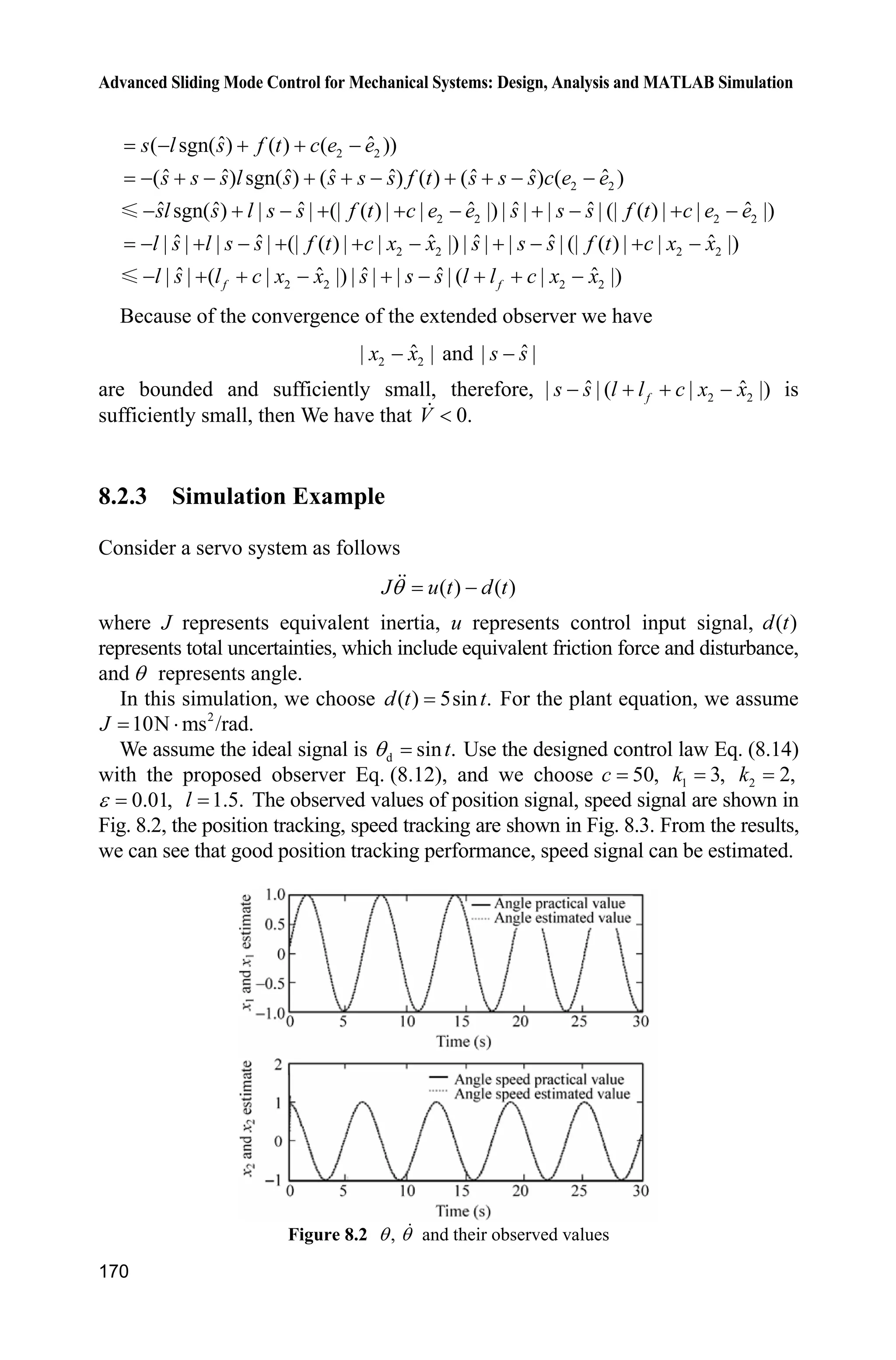
![8 Sliding Mode Control Based on Observer
167
(2) High gain observer: chap8_1obv.m
function [sys,x0,str,ts]=s_function(t,x,u,flag)
switch flag,
case 0,
[sys,x0,str,ts]=mdlInitializeSizes;
case 1,
sys=mdlDerivatives(t,x,u);
case 3,
sys=mdlOutputs(t,x,u);
case {2, 4, 9 }
sys = [];
otherwise
error(['Unhandled flag = ',num2str(flag)]);
end
function [sys,x0,str,ts]=mdlInitializeSizes
sizes = simsizes;
sizes.NumContStates = 2;
sizes.NumDiscStates = 0;
sizes.NumOutputs = 2;
sizes.NumInputs = 1;
sizes.DirFeedthrough = 1;
sizes.NumSampleTimes = 0;
sys=simsizes(sizes);
x0=[0 0];
str=[];
ts=[];
function sys=mdlDerivatives(t,x,u)
v=u(1);
alfa2=6;alfa1=9;
epc=0.01;
e=x(1)-v;
sys(1)=x(2)-alfa2/epc*e;
sys(2)=-alfa1/(epc^2)*e;
function sys=mdlOutputs(t,x,u)
sys(1)=x(1);
sys(2)=x(2);
(3) Plant program: chap8_1plant.m
function [sys,x0,str,ts]=s_function(t,x,u,flag)
switch flag,
case 0,
[sys,x0,str,ts]=mdlInitializeSizes;
case 1,
sys=mdlDerivatives(t,x,u);
case 3,
sys=mdlOutputs(t,x,u);
case {2, 4, 9 }
sys = [];
otherwise
error(['Unhandled flag = ',num2str(flag)]);](https://image.slidesharecdn.com/advancedslidingmodecontrolformechanicalsystems-130611121131-phpapp01/75/Advanced-sliding-mode-control-for-mechanical-systems-184-2048.jpg)
![Advanced Sliding Mode Control for Mechanical Systems: Design, Analysis and MATLAB Simulation
168
end
function [sys,x0,str,ts]=mdlInitializeSizes
sizes = simsizes;
sizes.NumContStates = 2;
sizes.NumDiscStates = 0;
sizes.NumOutputs = 2;
sizes.NumInputs = 1;
sizes.DirFeedthrough = 0;
sizes.NumSampleTimes = 0;
sys=simsizes(sizes);
x0=[0.05;0];
str=[];
ts=[];
function sys=mdlDerivatives(t,x,u)
a=25;
b=133;
ut=u(1);
dt=1*sign(x(2));
f=-a*x(2)-dt;
sys(1)=x(2);
sys(2)=f+b*ut;
function sys=mdlOutputs(t,x,u)
sys(1)=x(1);
sys(2)=x(2);
(4) Plot program: chap8_1plot.m
close all;
figure(1);
subplot(211);
plot(t,x(:,1),'k',t,x(:,3),'r:','linewidth',2);
xlabel('time(s)');ylabel('x1 and its estimate');
legend('ideal x1','estimate x1');
subplot(212);
plot(t,x(:,2),'k',t,x(:,4),'r:','linewidth',2);
xlabel('time(s)');ylabel('x2 and its estimate');
legend('ideal x2','estimate x2');
8.2 Sliding Mode Control Based on High Gain Observer
8.2.1 System Description
Consider the plant as
( ) ( )bu t f tT (8.10)
where T and T are position signal and speed signal respectively, u(t) is control](https://image.slidesharecdn.com/advancedslidingmodecontrolformechanicalsystems-130611121131-phpapp01/75/Advanced-sliding-mode-control-for-mechanical-systems-185-2048.jpg)
![8 Sliding Mode Control Based on Observer
171
Figure 8.3 Position and speed tracking with high gain observer
Matlab programs:
(1) Main Simulink: chap8_2sim.mdl
(2) Sliding mode control: chap8_2ctrl.m
function [sys,x0,str,ts]=s_function(t,x,u,flag)
switch flag,
case 0,
[sys,x0,str,ts]=mdlInitializeSizes;
case 3,](https://image.slidesharecdn.com/advancedslidingmodecontrolformechanicalsystems-130611121131-phpapp01/75/Advanced-sliding-mode-control-for-mechanical-systems-188-2048.jpg)
![Advanced Sliding Mode Control for Mechanical Systems: Design, Analysis and MATLAB Simulation
172
sys=mdlOutputs(t,x,u);
case {1,2, 4, 9 }
sys = [];
otherwise
error(['Unhandled flag = ',num2str(flag)]);
end
function [sys,x0,str,ts]=mdlInitializeSizes
sizes = simsizes;
sizes.NumContStates = 0;
sizes.NumDiscStates = 0;
sizes.NumOutputs = 1;
sizes.NumInputs = 5;
sizes.DirFeedthrough = 1;
sizes.NumSampleTimes = 0;
sys=simsizes(sizes);
x0=[];
str=[];
ts=[];
function sys=mdlOutputs(t,x,u)
r=u(1);
x1p=u(2);x2p=u(3);
x1=u(4);x2=u(5);
dr=cos(t);
ddr=-sin(t);
J=10;b=1/J;
c=50;
e1p=x1p-r;
e2p=x2p-dr;
sp=e2p+c*e1p;
delta=0.15;
kk=1/delta;
if spdelta
sat_sp=1;
elseif abs(sp)=delta
sat_sp=kk*sp;
elseif sp-delta
sat_sp=-1;
end
M=2;
l=1.50; %l=5/10;
if M==1
ut=1/b*(ddr-c*e2p-l*sign(sp));
elseif M==2
ut=1/b*(ddr-c*e2p-l*sat_sp);](https://image.slidesharecdn.com/advancedslidingmodecontrolformechanicalsystems-130611121131-phpapp01/75/Advanced-sliding-mode-control-for-mechanical-systems-189-2048.jpg)
![8 Sliding Mode Control Based on Observer
173
end
sys(1)=ut;
(3) Plant program: chap8_2plant.m
function [sys,x0,str,ts]=s_function(t,x,u,flag)
switch flag,
case 0,
[sys,x0,str,ts]=mdlInitializeSizes;
case 1,
sys=mdlDerivatives(t,x,u);
case 3,
sys=mdlOutputs(t,x,u);
case {2, 4, 9 }
sys = [];
otherwise
error(['Unhandled flag = ',num2str(flag)]);
end
function [sys,x0,str,ts]=mdlInitializeSizes
sizes = simsizes;
sizes.NumContStates = 2;
sizes.NumDiscStates = 0;
sizes.NumOutputs = 2;
sizes.NumInputs = 1;
sizes.DirFeedthrough = 0;
sizes.NumSampleTimes = 0;
sys=simsizes(sizes);
x0=[0.1;0];
str=[];
ts=[];
function sys=mdlDerivatives(t,x,u)
J=10;
ut=u(1);
d=5.0*sin(t);
sys(1)=x(2);
sys(2)=1/J*(ut-d);
function sys=mdlOutputs(t,x,u)
sys(1)=x(1);
sys(2)=x(2);
(4) Plot program: chap8_2plot.m
close all;
figure(1);
subplot(211);
plot(t,y(:,1),'k',t,y(:,3),'r:','linewidth',2);
xlabel('time(s)');ylabel('Position tracking');
legend('ideal angle signal','practical angle signal');
subplot(212);
plot(t,y(:,2),'k',t,y(:,4),'r:','linewidth',2);](https://image.slidesharecdn.com/advancedslidingmodecontrolformechanicalsystems-130611121131-phpapp01/75/Advanced-sliding-mode-control-for-mechanical-systems-190-2048.jpg)
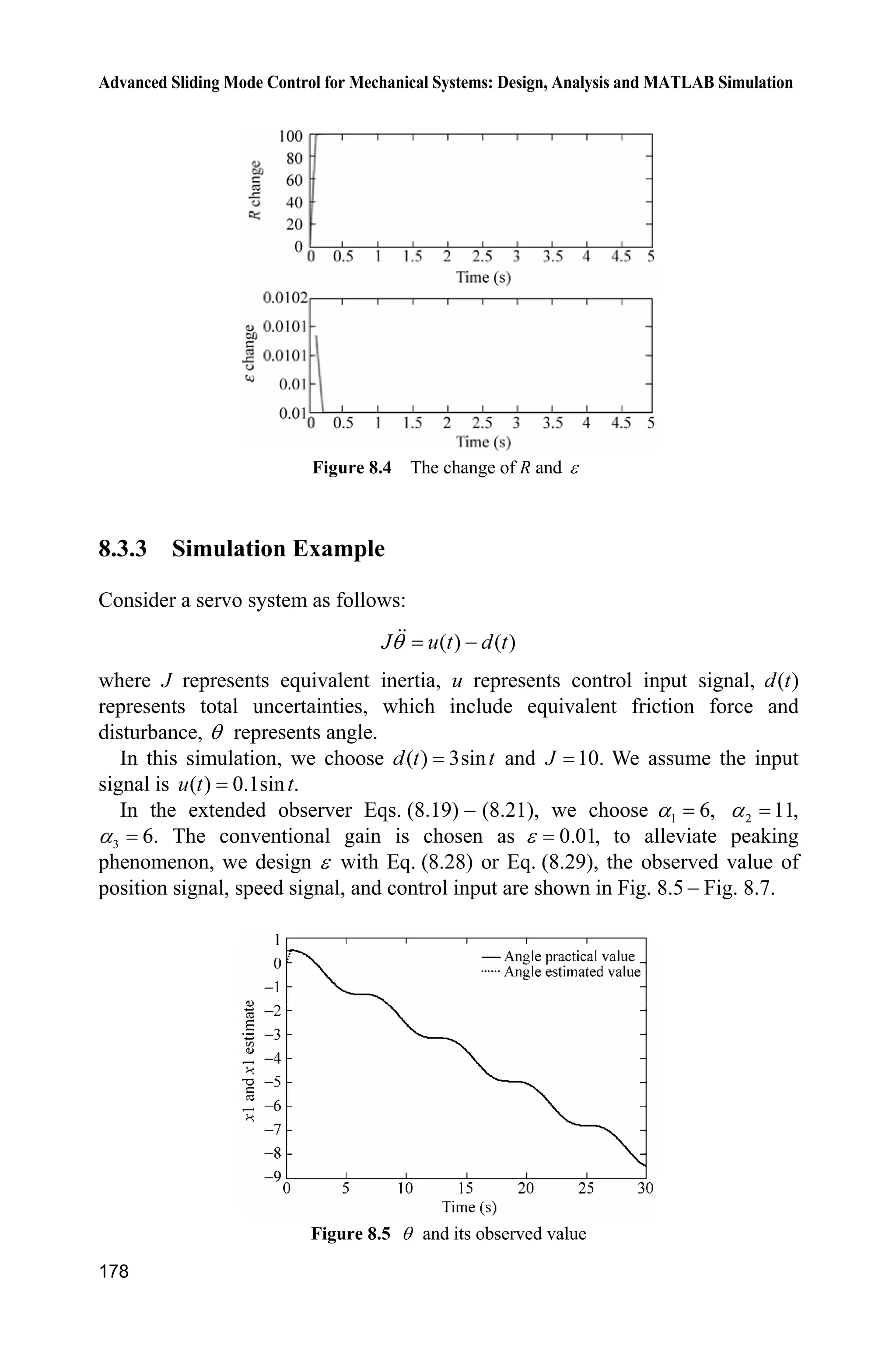
![8 Sliding Mode Control Based on Observer
175
8.3.2 Extended State Observer Design
Refer to [3], the extended state observer is designed as follows:
1
1 2 1
ˆ ˆ ˆ( )x x y x
D
H
(8.19)
2
2 12
ˆ ˆ ˆ( )x bu y x
D
V
H
(8.20)
3
13
ˆ ˆ( )y x
D
V
H
(8.21)
The goals of the observer are that
1 1 2 2 3
ˆ ˆ ˆ( ) ( ), ( ) ( ), ( ) ( , , )T To o ox t x t x t x t x t f t as .t o f
where 1
ˆx , 2
ˆx and ˆV are states of the observer, 0,H ! 1D , 2D and 3D are positive
constants, polynomial 3 2
1 2 3s s sD D D is Hurwitz.
Refer to [4], we define observer error as
@
T
1 2 3K K KK
where
1 1 2 2
1 2 32
ˆ ˆ
ˆ, ,
x x x x
fK K K V
H H
Since
1 1 1
1 2 2 1
1 1
2 2 1 1 1 2 2 1 1 22
ˆ 1
ˆ ˆ( )
1 1
ˆ ˆ ˆ ˆ( ) ( ) ( )
x x
x x y x
x x y x x x x x
D
HK
H H H
D D
D K K
H H H H
§ ·§ ·
¨ ¸¨ ¸
© ¹© ¹
§ ·
¨ ¸
© ¹
2 2 2
2 12
2 2
1 1 1 2 1 32 2
ˆ
ˆ ˆ( ) ( )
ˆ ˆ ˆ ˆ( ) ( ) ( ) ( )
x x
bu f bu y x
f y x x x f
D
HK H V
H H
D D
V V D K K
H H
§ ·§ ·
˜ ¨ ¸¨ ¸
© ¹© ¹
§ ·
˜ ¨ ¸
© ¹
3 3
3 1 1 3 13 2
ˆ ˆ ˆ( ) ( ) ( )f f y x f y x f
D D
HK H V H H D K H
H H
§ ·
¨ ¸
© ¹](https://image.slidesharecdn.com/advancedslidingmodecontrolformechanicalsystems-130611121131-phpapp01/75/Advanced-sliding-mode-control-for-mechanical-systems-192-2048.jpg)
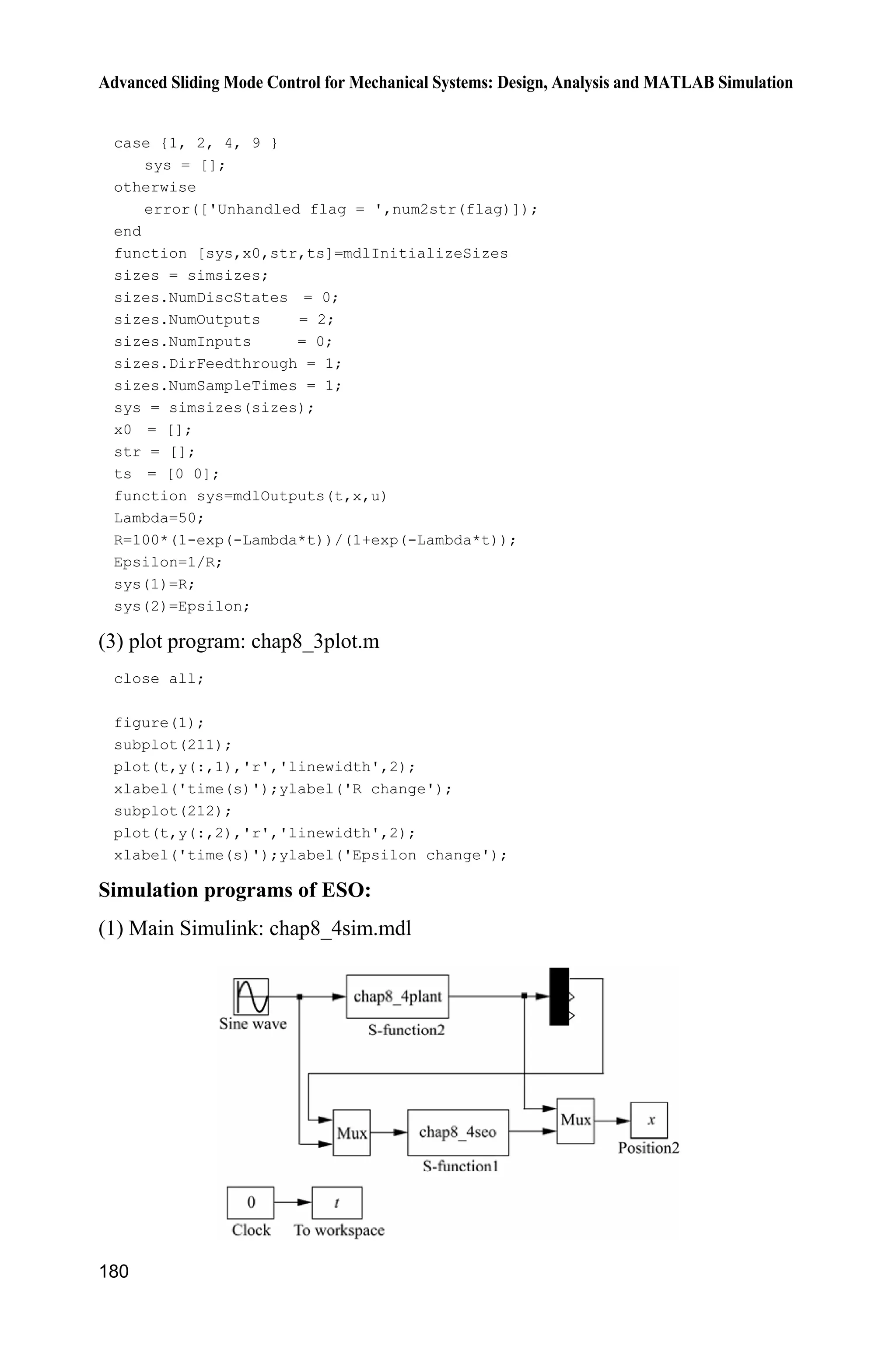
![8 Sliding Mode Control Based on Observer
177
and
2
o min ( ) || || 2 || |||| ||V LO H Q PBK K (8.26)
where min ( )O Q is the minimum eigenvalue of Q.
From o 0,V we get observer error convergence conclusion as
min
2 || ||
|| ||
( )
LH
O
PB
Q
K (8.27)
From Eq. (8.27), we can see the convergence of observer error K is related
to .H If H is designed as very positive small, || ||K is ( ).O H
Remark:
(1) If the initial value of the extended observer and the initial value of the plant
is different, for very small H , peaking phenomenon will appear, which can affect
convergence of the extended observer greatly. To alleviate peaking phenomenon,
we design H as [5]
3
100 , 0 11
100, 1
t t
R
tH
®
!¯
(8.28)
or
1
2
max
max
1 e
, 01
1 e
,
t
t
t t
R
t t
O
O
P
H
P
°
®
° !¯
(8.29)
where ,P 1O and 2O are positive value.
For example, choose 1 2 50,O O 100,P run simulink program chap8_3sim.mdl,
the change of R and H are shown in Fig. 8.4.
(2) If the practical measurement signal is mixed with noise, for very small ,H
big observer error can be caused. To alleviate the effect of noisy signal, a switched-
gain can be used in the observer[6]
.
(3) Design of ( 1,2,3).i iD For 3 2
1 2 3 0,O D O D O D we choose ( 1)(O O
2)( 3) 0,O then 3 2
6 11 6 0,O O O we can get 1 6,D 2 11D , 3 6.D](https://image.slidesharecdn.com/advancedslidingmodecontrolformechanicalsystems-130611121131-phpapp01/75/Advanced-sliding-mode-control-for-mechanical-systems-194-2048.jpg)
![8 Sliding Mode Control Based on Observer
179
Figure 8.6 T and its observed value
Figure 8.7 Total uncertainty and its observed value
Simulation programs of peak supression function:
(1) Simulink program: chap8_3sim.mdl
(2) S-function of peak program: chap8_3.m
function [sys,x0,str,ts]=s_function(t,x,u,flag)
switch flag,
case 0,
[sys,x0,str,ts]=mdlInitializeSizes;
case 3,
sys=mdlOutputs(t,x,u);](https://image.slidesharecdn.com/advancedslidingmodecontrolformechanicalsystems-130611121131-phpapp01/75/Advanced-sliding-mode-control-for-mechanical-systems-196-2048.jpg)
![Advanced Sliding Mode Control for Mechanical Systems: Design, Analysis and MATLAB Simulation
180
case {1, 2, 4, 9 }
sys = [];
otherwise
error(['Unhandled flag = ',num2str(flag)]);
end
function [sys,x0,str,ts]=mdlInitializeSizes
sizes = simsizes;
sizes.NumDiscStates = 0;
sizes.NumOutputs = 2;
sizes.NumInputs = 0;
sizes.DirFeedthrough = 1;
sizes.NumSampleTimes = 1;
sys = simsizes(sizes);
x0 = [];
str = [];
ts = [0 0];
function sys=mdlOutputs(t,x,u)
Lambda=50;
R=100*(1-exp(-Lambda*t))/(1+exp(-Lambda*t));
Epsilon=1/R;
sys(1)=R;
sys(2)=Epsilon;
(3) plot program: chap8_3plot.m
close all;
figure(1);
subplot(211);
plot(t,y(:,1),'r','linewidth',2);
xlabel('time(s)');ylabel('R change');
subplot(212);
plot(t,y(:,2),'r','linewidth',2);
xlabel('time(s)');ylabel('Epsilon change');
Simulation programs of ESO:
(1) Main Simulink: chap8_4sim.mdl](https://image.slidesharecdn.com/advancedslidingmodecontrolformechanicalsystems-130611121131-phpapp01/75/Advanced-sliding-mode-control-for-mechanical-systems-197-2048.jpg)
![8 Sliding Mode Control Based on Observer
181
(2) Extended observer: chap8_4eso.m
function [sys,x0,str,ts]=s_function(t,x,u,flag)
switch flag,
case 0,
[sys,x0,str,ts]=mdlInitializeSizes;
case 1,
sys=mdlDerivatives(t,x,u);
case 3,
sys=mdlOutputs(t,x,u);
case {2, 4, 9 }
sys = [];
otherwise
error(['Unhandled flag = ',num2str(flag)]);
end
function [sys,x0,str,ts]=mdlInitializeSizes
sizes = simsizes;
sizes.NumContStates = 3;
sizes.NumDiscStates = 0;
sizes.NumOutputs = 3;
sizes.NumInputs = 2;
sizes.DirFeedthrough = 1;
sizes.NumSampleTimes = 0;
sys=simsizes(sizes);
x0=[0 0 0];
str=[];
ts=[];
function sys=mdlDerivatives(t,x,u)
y=u(1);
ut=u(2);
J=10;
b=1/J;
alfa1=6;alfa2=11;alfa3=6;
M=1;
if M==1
epc=0.01;
elseif M==2
if t=1;
R=100*t^3;
elseif t1;
R=100;
end
epc=1/R;
elseif M==3
nmn=0.1;
R=100*(1-exp(-nmn*t))/(1+exp(-nmn*t));](https://image.slidesharecdn.com/advancedslidingmodecontrolformechanicalsystems-130611121131-phpapp01/75/Advanced-sliding-mode-control-for-mechanical-systems-198-2048.jpg)
![Advanced Sliding Mode Control for Mechanical Systems: Design, Analysis and MATLAB Simulation
182
epc=1/R;
end
e=y-x(1);
sys(1)=x(2)+alfa1/epc*e;
sys(2)=b*ut+x(3)+alfa2/epc^2*e;
sys(3)=alfa3/epc^3*e;
function sys=mdlOutputs(t,x,u)
sys(1)=x(1);
sys(2)=x(2);
sys(3)=x(3);
(3) Plant program: chap8_4plant.m
function [sys,x0,str,ts]=s_function(t,x,u,flag)
switch flag,
case 0,
[sys,x0,str,ts]=mdlInitializeSizes;
case 1,
sys=mdlDerivatives(t,x,u);
case 3,
sys=mdlOutputs(t,x,u);
case {2, 4, 9 }
sys = [];
otherwise
error(['Unhandled flag = ',num2str(flag)]);
end
function [sys,x0,str,ts]=mdlInitializeSizes
sizes = simsizes;
sizes.NumContStates = 2;
sizes.NumDiscStates = 0;
sizes.NumOutputs = 3;
sizes.NumInputs = 1;
sizes.DirFeedthrough = 0;
sizes.NumSampleTimes = 0;
sys=simsizes(sizes);
x0=[0.5;0];
str=[];
ts=[];
function sys=mdlDerivatives(t,x,u)
J=10;
ut=u(1);
d=3.0*sin(t);
sys(1)=x(2);
sys(2)=1/J*(ut-d);
function sys=mdlOutputs(t,x,u)
J=10;
d=3.0*sin(t);](https://image.slidesharecdn.com/advancedslidingmodecontrolformechanicalsystems-130611121131-phpapp01/75/Advanced-sliding-mode-control-for-mechanical-systems-199-2048.jpg)
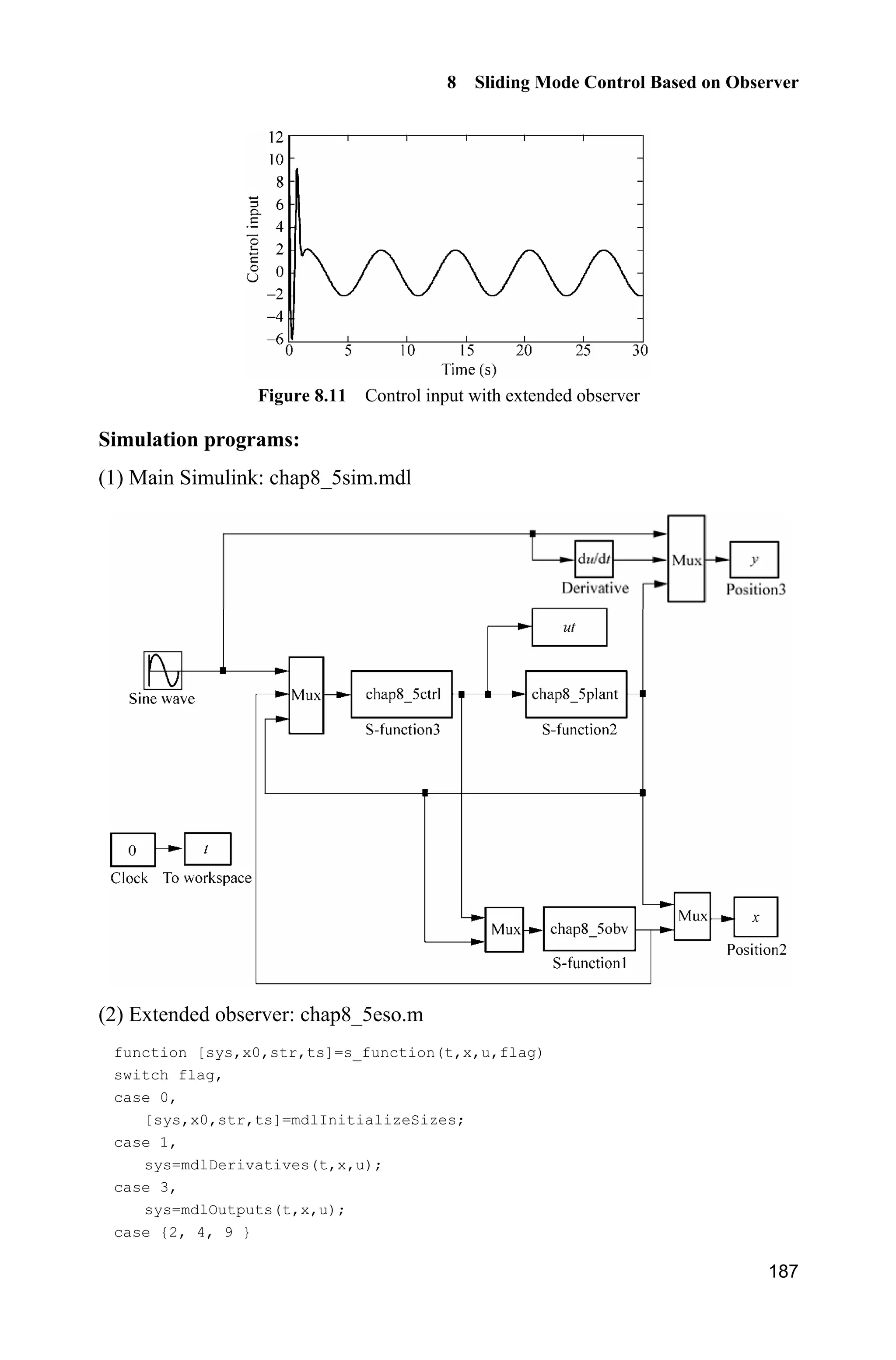
![8 Sliding Mode Control Based on Observer
187
Figure 8.11 Control input with extended observer
Simulation programs:
(1) Main Simulink: chap8_5sim.mdl
(2) Extended observer: chap8_5eso.m
function [sys,x0,str,ts]=s_function(t,x,u,flag)
switch flag,
case 0,
[sys,x0,str,ts]=mdlInitializeSizes;
case 1,
sys=mdlDerivatives(t,x,u);
case 3,
sys=mdlOutputs(t,x,u);
case {2, 4, 9 }](https://image.slidesharecdn.com/advancedslidingmodecontrolformechanicalsystems-130611121131-phpapp01/75/Advanced-sliding-mode-control-for-mechanical-systems-204-2048.jpg)
![Advanced Sliding Mode Control for Mechanical Systems: Design, Analysis and MATLAB Simulation
188
sys = [];
otherwise
error(['Unhandled flag = ',num2str(flag)]);
end
function [sys,x0,str,ts]=mdlInitializeSizes
sizes = simsizes;
sizes.NumContStates = 3;
sizes.NumDiscStates = 0;
sizes.NumOutputs = 3;
sizes.NumInputs = 4;
sizes.DirFeedthrough = 1;
sizes.NumSampleTimes = 0;
sys=simsizes(sizes);
x0=[0 0 0];
str=[];
ts=[];
function sys=mdlDerivatives(t,x,u)
ut=u(1);
y=u(2);
b=0.1;
alfa1=6;alfa2=11;alfa3=6;
M=3;
if M==1
epc=0.01;
elseif M==2
if t=1;
R=100*t^3;
elseif t1;
R=100;
end
epc=1/R;
elseif M==3
nmn=0.1;
R=100*(1-exp(-nmn*t))/(1+exp(-nmn*t));
epc=1/R;
end
e=y-x(1);
sys(1)=x(2)+alfa1/epc*e;
sys(2)=b*ut+x(3)+alfa2/epc^2*e;
sys(3)=alfa3/epc^3*e;
function sys=mdlOutputs(t,x,u)
sys(1)=x(1);
sys(2)=x(2);
sys(3)=x(3);
(3) Controller program: chap8_5ctrl.m
function [sys,x0,str,ts]=s_function(t,x,u,flag)
switch flag,](https://image.slidesharecdn.com/advancedslidingmodecontrolformechanicalsystems-130611121131-phpapp01/75/Advanced-sliding-mode-control-for-mechanical-systems-205-2048.jpg)
![8 Sliding Mode Control Based on Observer
189
case 0,
[sys,x0,str,ts]=mdlInitializeSizes;
case 3,
sys=mdlOutputs(t,x,u);
case {1,2, 4, 9 }
sys = [];
otherwise
error(['Unhandled flag = ',num2str(flag)]);
end
function [sys,x0,str,ts]=mdlInitializeSizes
sizes = simsizes;
sizes.NumContStates = 0;
sizes.NumDiscStates = 0;
sizes.NumOutputs = 1;
sizes.NumInputs = 7;
sizes.DirFeedthrough = 1;
sizes.NumSampleTimes = 0;
sys=simsizes(sizes);
x0=[];
str=[];
ts=[];
function sys=mdlOutputs(t,x,u)
r=u(1);
x1p=u(2);x2p=u(3);x3p=u(4);
x1=u(5);x2=u(6);
dr=0.1*cos(t);
ddr=-0.1*sin(t);
b=0.1;c=10;l=0.5;
e1p=x1p-r;
e2p=x2p-dr;
sp=e2p+c*e1p;
ut=1/b*(-x3p+ddr-c*e2p-l*sign(sp)); %With Extended Observer
delta=0.15;
kk=1/delta;
if spdelta
sat_sp=1;
elseif abs(sp)=delta
sat_sp=kk*sp;
elseif sp-delta
sat_sp=-1;
end
ut=1/b*(-x3p+ddr-c*e2p-l*sat_sp); %With Extended Observer
sys(1)=ut;
(4) Plant program: chap8_5plant.m
function [sys,x0,str,ts]=s_function(t,x,u,flag)
switch flag,
case 0,](https://image.slidesharecdn.com/advancedslidingmodecontrolformechanicalsystems-130611121131-phpapp01/75/Advanced-sliding-mode-control-for-mechanical-systems-206-2048.jpg)
![Advanced Sliding Mode Control for Mechanical Systems: Design, Analysis and MATLAB Simulation
190
[sys,x0,str,ts]=mdlInitializeSizes;
case 1,
sys=mdlDerivatives(t,x,u);
case 3,
sys=mdlOutputs(t,x,u);
case {2, 4, 9 }
sys = [];
otherwise
error(['Unhandled flag = ',num2str(flag)]);
end
function [sys,x0,str,ts]=mdlInitializeSizes
sizes = simsizes;
sizes.NumContStates = 2;
sizes.NumDiscStates = 0;
sizes.NumOutputs = 3;
sizes.NumInputs = 1;
sizes.DirFeedthrough = 0;
sizes.NumSampleTimes = 0;
sys=simsizes(sizes);
x0=[0.1;0];
str=[];
ts=[];
function sys=mdlDerivatives(t,x,u)
b=0.10;
f=0.3*sin(t);
ut=u(1);
sys(1)=x(2);
sys(2)=b*ut+f;
function sys=mdlOutputs(t,x,u)
b=0.10;
f=0.3*sin(t);
sys(1)=x(1);
sys(2)=x(2);
sys(3)=f;
(5) Plot program: chap8_5plot.m
close all;
figure(1);
plot(t,y(:,1),'k',t,y(:,3),'r:','linewidth',2);
xlabel('time(s)');ylabel('Position tracking');
legend('ideal signal','practical signal');
figure(2);
plot(t,y(:,2),'k',t,y(:,4),'r:','linewidth',2);
xlabel('time(s)');ylabel('speed tracking');
legend('angle speed ideal signal','angle speed practical signal');
figure(3);
plot(t,ut(:,1),'k','linewidth',2);
xlabel('time(s)');ylabel('control input');](https://image.slidesharecdn.com/advancedslidingmodecontrolformechanicalsystems-130611121131-phpapp01/75/Advanced-sliding-mode-control-for-mechanical-systems-207-2048.jpg)
![8 Sliding Mode Control Based on Observer
191
(6) Plot program of ESO: chap8_5eso_plot.m
close all;
figure(1);
plot(t,x(:,1),'k',t,x(:,4),'r:','linewidth',2);
xlabel('time(s)');ylabel('x1 and x1 estimate');
legend('angle practical value','angle estimated value');
figure(2);
plot(t,x(:,2),'k',t,x(:,5),'r:','linewidth',2);
xlabel('time(s)');ylabel('x2 and x2 estimate');
legend('angle speed practical value','angle speed estimated value');
figure(3);
plot(t,x(:,3),'k',t,x(:,6),'r:','linewidth',2);
xlabel('time(s)');ylabel('x3 and x3 estimate');
legend('ft practical value','ft estimated value');
8.5 Universal Approximation Using High-Order
Integral-Chain Differentiator
8.5.1 System Description
Consider n-order nonlinear system as follow:
1 2
2 3
1
1
( ) ( )
n n
n
x x
x x
x x
x f g u
y x
½
°
°
°°
¾
°
°
°
°¿
x x
#
(8.36)
where T
1 2[ ]nx x xx is the state vector, f and g are all nonlinear functions,
u R and y R are the input control and output respectively. Function g(x) is
bounded.
8.5.2 Integral-Chain Differentiator
For the system (8.36), we suppose that ( )f x is uncertain and 2 3, , , nx x x are
unknown. We give the following estimation theorem.](https://image.slidesharecdn.com/advancedslidingmodecontrolformechanicalsystems-130611121131-phpapp01/75/Advanced-sliding-mode-control-for-mechanical-systems-208-2048.jpg)
![Advanced Sliding Mode Control for Mechanical Systems: Design, Analysis and MATLAB Simulation
192
Theorem 1: For the system (8.36), we design the following integral-chain
differentiator[5]
:
1 2
2 3
1
1
11 2
1 1 1 2 11 2
ˆ ˆ
ˆ ˆ
ˆ ˆ
ˆ ˆ
ˆ ˆ ˆ ˆ ˆ( )
n n
n n
n n
n n nn n
x x
x x
x x
x x
a aa a
x x x x x x
H H H H
½
°
°
°
°°
¾
°
°
°
°
°¿
#
(8.37)
to approximate ( )f x and estimate 2 3, , , nx x x from the output 1y x and input
u of the system (8.36). Where 0H ! perturbation parameter which is sufficiently
small. 1
1 2 1 0n n
ns a s a s a
is Hurwitz. Therefore, we have that
0
ˆlim , 1,2, ,i ix x i n
H o
(8.38)
and
1
0
ˆlim ( ) ( )nx f g u
H
o
x x or 1
0
ˆˆ( ) lim( ( ) )nf t x g u
H
o
x (8.39)
where
1 2
ˆ ˆ ˆ ˆ[ ]nx x x 7
x
Proof: The Laplace transformation of the integral-chain differentiator (8.37) is
ˆ ( )ˆ ( ) , 0,1, , 1; 1,2, , 1 i
i k k
X s
X s k i i n
s
(8.40)
1 2 1 1
1 1 2 1 12 1 1
ˆ ˆ ˆ ˆ ˆ( ) ( ) ( ) ( ) ( ) ( )n n
n n n n n n
a a a a a
sX s X s X s X s X s X s
H H H H H
(8.41)
where ˆ ( )iX s is the Laplace transformation of ˆ ( ),ix t 1,2, , 1.i n
From Eqs. (8.39) and (8.40), we have
1 2 1 1
1
2
1 1 2 1
1 1 12 1
ˆ ( ) ( )
1,2, ,
n n i n n i n n i
n n
i
i i i
i i ii i
s a s a s
a a a
a s a X s a X s
s s s
i n
H H H
H H
H H
§
¨
©
·
¸
¹
(8.42)](https://image.slidesharecdn.com/advancedslidingmodecontrolformechanicalsystems-130611121131-phpapp01/75/Advanced-sliding-mode-control-for-mechanical-systems-209-2048.jpg)
![8 Sliding Mode Control Based on Observer
193
Therefore, we get
1
0
1
ˆ ( )
lim , 1,2, , 1
( )
iiX s
s i n
X sH
o
(8.43)
Accordingly, we get Eq. (8.38). Moreover, from Eq. (8.37), we have
1
0
ˆlim n nx x
H
o
From ( ) ( )nx f g ux x in Eq. (8.36), we can get Eq. (8.39).
This concludes the proof.
Remark: From Eq. (8.41), we get
1
1
1
1 1 2 11
2 1
ˆ ( )
( )
n
n n nn n
n n
a
X s
a a a aX s
s s s s
H
H H H H
We know that if the selection of 1 2 1, , , na a a is suitable, the filtering ability can
be obtained.
8.5.3 Simulation Example
Consider the following inverted pendulum:
1 2
2
1 2 1 1 c 1 c
2 2 2
1 c 1 c
sin cos sin /( ) cos /( )
(4/3 cos /( )) (4/3 cos /( ))
x x
g x mlx x x m m x m m
x u
l m x m m l m x m m
°
®
° ¯
where 1x and 2x are the swing angle and swing rate respectively. 2
9.8 m/s ,g
c 1 kgm is the vehicle mass, 0.1 kgm is the mass of pendulum. 0.5 ml is
one half of the pendulum length, and u is the control input.
From Eq. (8.37), the integral-chain differentiator is designed as
1 2
2 3
31 2
3 1 1 2 33 2
ˆ ˆ
ˆ ˆ
ˆ ˆ ˆ ˆ( )
x x
x x
aa a
x x x x x
H H H
where 0.01,H 1 2 3 10.a a a The input signal is ( ) 0.1sin ,u t t the initial
state is [ / 60 0].S The curves of position tracking, velocity estimation and
uncertainty approximation using integral-chain differentiator are in Fig. 8.12
Fig. 8.14.](https://image.slidesharecdn.com/advancedslidingmodecontrolformechanicalsystems-130611121131-phpapp01/75/Advanced-sliding-mode-control-for-mechanical-systems-210-2048.jpg)
![8 Sliding Mode Control Based on Observer
195
Simulation programs:
(1) Main Simulink program: chap8_6sim.mdl
(2) TD differentiator program: chap8_6TD.m
function [sys,x0,str,ts] = Differentiator(t,x,u,flag)
switch flag,
case 0,
[sys,x0,str,ts]=mdlInitializeSizes;
case 1,
sys=mdlDerivatives(t,x,u);
case 3,
sys=mdlOutputs(t,x,u);
case {2, 4, 9 }
sys = [];
otherwise
error(['Unhandled flag = ',num2str(flag)]);
end
function [sys,x0,str,ts]=mdlInitializeSizes
sizes = simsizes;
sizes.NumContStates = 3;
sizes.NumDiscStates = 0;
sizes.NumOutputs = 3;
sizes.NumInputs = 1;
sizes.DirFeedthrough = 1;
sizes.NumSampleTimes = 1;
sys = simsizes(sizes);
x0 = [0 0 0];
str = [];
ts = [0 0];
function sys=mdlDerivatives(t,x,u)
vt=u(1);](https://image.slidesharecdn.com/advancedslidingmodecontrolformechanicalsystems-130611121131-phpapp01/75/Advanced-sliding-mode-control-for-mechanical-systems-212-2048.jpg)
![Advanced Sliding Mode Control for Mechanical Systems: Design, Analysis and MATLAB Simulation
196
epc=0.01;
alfa1=1;
alfa2=3;
alfa3=3;
e=x(1)-vt;
sys(1)=x(2);
sys(2)=x(3);
sys(3)=-alfa1/epc^3*e-alfa2/epc^2*x(2)-alfa3/epc*x(3);
function sys=mdlOutputs(t,x,u)
sys = x;
(3) Plant program: chap8_6plant.m
function [sys,x0,str,ts]=s_function(t,x,u,flag)
switch flag,
case 0,
[sys,x0,str,ts]=mdlInitializeSizes;
case 1,
sys=mdlDerivatives(t,x,u);
case 3,
sys=mdlOutputs(t,x,u);
case {2, 4, 9 }
sys = [];
otherwise
error(['Unhandled flag = ',num2str(flag)]);
end
function [sys,x0,str,ts]=mdlInitializeSizes
sizes = simsizes;
sizes.NumContStates = 2;
sizes.NumDiscStates = 0;
sizes.NumOutputs = 3;
sizes.NumInputs = 1;
sizes.DirFeedthrough = 0;
sizes.NumSampleTimes = 0;
sys=simsizes(sizes);
x0=[pi/60 0];
str=[];
ts=[];
function sys=mdlDerivatives(t,x,u)
g=9.8;mc=1.0;m=0.1;l=0.5;
S=l*(4/3-m*(cos(x(1)))^2/(mc+m));
fx=g*sin(x(1))-m*l*x(2)^2*cos(x(1))*sin(x(1))/(mc+m);
fx=fx/S;
gx=cos(x(1))/(mc+m);
gx=gx/S;
sys(1)=x(2);](https://image.slidesharecdn.com/advancedslidingmodecontrolformechanicalsystems-130611121131-phpapp01/75/Advanced-sliding-mode-control-for-mechanical-systems-213-2048.jpg)
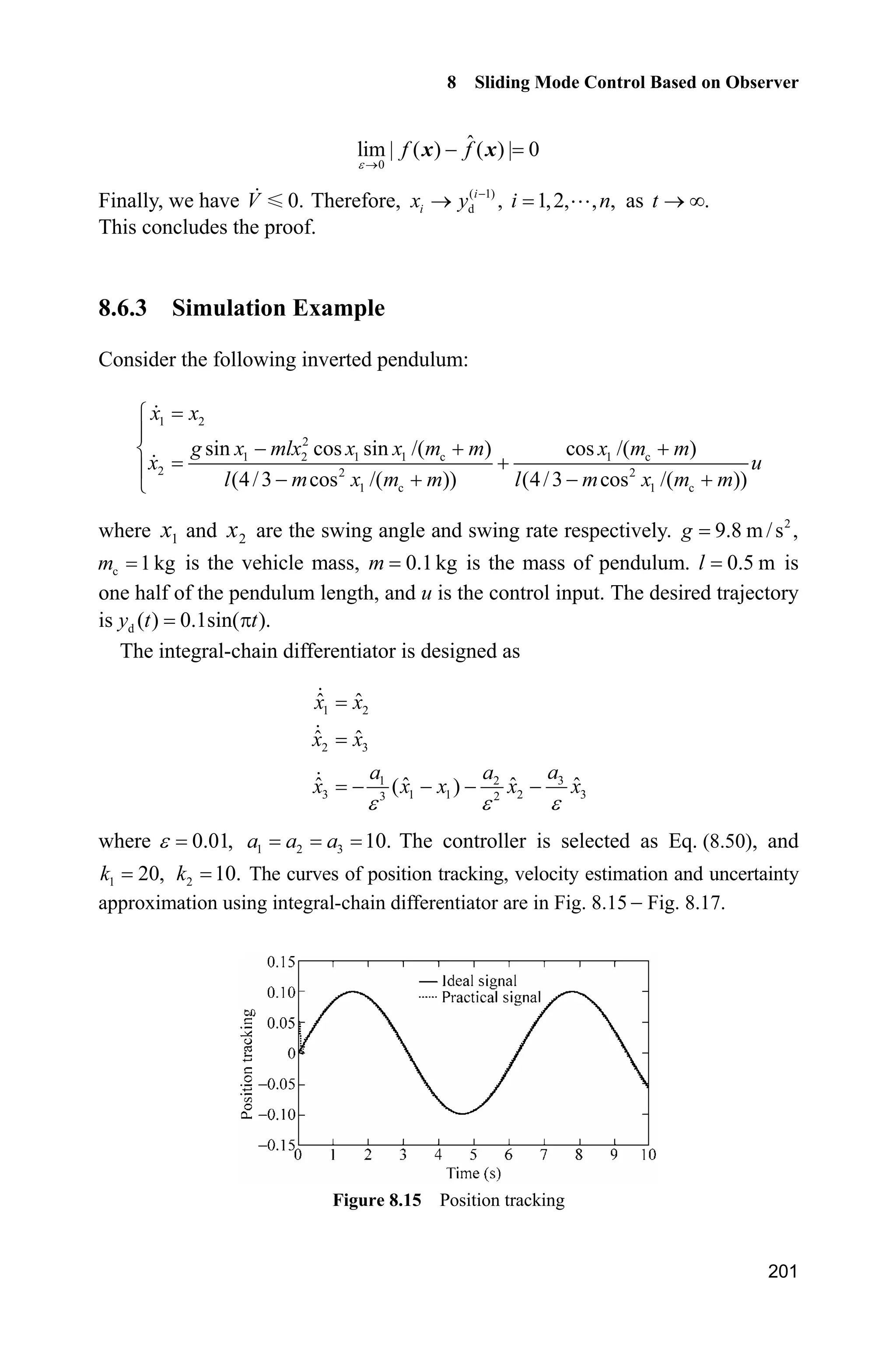
![Advanced Sliding Mode Control for Mechanical Systems: Design, Analysis and MATLAB Simulation
198
Let
(1) ( 1)
1 2 1 d 2 d d
ˆ ˆ ˆ ˆ ˆ ˆ ˆ[ ] [ ]7 7
n
n ne e e x y x y x ye
We select a bounded controller u, i.e.,
| | uu l
Let
1
ˆ ˆˆ( ) ( )nf x g u x x (8.45)
and ( 1)
d
ˆ ˆ , 1,2, , .i
i ie x y i n
From Eq. (8.36), we have
( ) ( )nf x g ux x
Therefore, we have
1
ˆ ˆˆ( ) ( ) ( ( ) ( ))n nf f x x g g u x x x x
Therefore,
1
ˆ ˆˆ| ( ) ( ) | | | | ( ) ( ) || |n nf f x x g g u x x x x
For bounded u, we suppose exist constant gl such that
ˆ ˆ| ( ) ( ) | || ||gg g l x x x x (8.46)
Therefore, we get
1
ˆ ˆˆ| ( ) ( ) | | | || ||n n u gf f x x l l x x x x (8.47)
For system (8.36), we will design a controller based on integral-chain differentiator
to track desired trajectory, and given the following Theorem. Firstly, we can suppose
( )
1 d 1 1 2
ˆ ˆ ˆ| |n
n n nx y c e c e is bounded[7]
, i.e.
( ) T
d 1
ˆ ˆ| ( ) |n
f y l x C e (8.48)
where T
1 2 1[ ] ,n nc c c C T
1 2
ˆ ˆ ˆ ˆ[ ]n ne e ee and
inf sup( )l g lx (8.49)
8.6.2 Design of Sliding Mode Controller
The sliding variable:
1
1 1 1 1 1
n
n n n
d
s c e e c e c e
dt
§ ·
¨ ¸
© ¹](https://image.slidesharecdn.com/advancedslidingmodecontrolformechanicalsystems-130611121131-phpapp01/75/Advanced-sliding-mode-control-for-mechanical-systems-215-2048.jpg)

![Advanced Sliding Mode Control for Mechanical Systems: Design, Analysis and MATLAB Simulation
200
Therefore,
1
2
( )
d 1 1 2
1 1
2 2
ˆ ˆ ˆ ˆ ˆ ˆ( ( ) ( )) ( ) sgn( ) ( ) sgn( )
ˆ( ) ( ) ˆ ˆ ˆ ˆ( ( ) sgn( ))
ˆ( )
ˆ ˆˆ ˆ ˆ ˆ ˆ ˆ( ( ) ( )) ( )( ( ) ( )) ( ) ( ) ( )
( )
¦
¦ ¦
n
i i i
i
n
n n
n n
i i i i i i
i i
V s f f s c x x sl s s s l s
g g
s f y c e c e l s
g
s f f s s f f s c x x s s c x x
g
x x
x x
x
x
x x x x
x ( )
d 1 1 2
( )
d 1 1 2
ˆ( ) ˆˆ ˆ ˆ ˆ( ( ) sgn( ))
ˆ( )
ˆ( ) ( ) ˆˆ ˆ ˆ ˆ( )[ ( ) sgn( )]
ˆ( )
ˆ ˆ ˆ ˆsgn( ) ( ) sgn( )
n
n n
n
n n
g
s f y c e c e l s
g
g g
s s f x y c e c e l s
g
sl s s s l s
x
x
x
x x
x
Therefore, we have
1
2
( )
1 d 1
2
( )
1 2 d 1
ˆ ˆˆ ˆ ˆ ˆ( ) ( ) | || ( ) ( ) | | | | || |
ˆ| ( ) ( ) | ˆˆ ˆ ˆ ˆ| | | || | | || ( )
ˆ| ( ) |
ˆ| ( ) ( ) | ˆˆ ˆ ˆ ˆsgn( ) | | || ( )
ˆ| ( ) |
¦
¦
n
i i i
i
n
n
i i i n n
i
n
n n
V f f s s s f f s c x x
g g
s s c x x s f y c e
g
g g
c e l s s s f y c e
g
x x x x
x x
x
x
x x
x
x
1 2
1
2
g ( )
1 d 1
2 inf
g
1 2
inf
ˆ ˆ ˆ ˆsgn( ) | | | | |
ˆ ˆˆ ˆ ˆ ˆ( ) ( ) | || ( ) ( ) | | | | || |
ˆ| | ˆˆ ˆ ˆ ˆ| | | || | | || ( )
ˆ| | ˆˆ ˆ ˆsgn( ) | | || ( )
¦
¦
n
i i i
i
n
n
i i i n n
i
c e l s l s s l s
f f s s s f f s c x x
l x x
s s c x x s f y c e
l
l
c e l s s s f y
l
x x x x
x
x x
x ( )
d 1
1 2
ˆ
ˆ ˆ ˆ ˆsgn( ) | | | | |
n
n nc e
c e l s l s s l s
When H is sufficient small, we have
0
ˆlim | | 0,s s
H o
0
ˆlim | | 0,i ix x
H o
1
0
ˆlim | | 0n nx x
H
o
and from Eq. (8.47), we have](https://image.slidesharecdn.com/advancedslidingmodecontrolformechanicalsystems-130611121131-phpapp01/75/Advanced-sliding-mode-control-for-mechanical-systems-217-2048.jpg)
![8 Sliding Mode Control Based on Observer
203
(2) Sliding mode controller: chap8_7ctrl.m
function [sys,x0,str,ts] = spacemodel(t,x,u,flag)
switch flag,
case 0,
[sys,x0,str,ts]=mdlInitializeSizes;
case 3,
sys=mdlOutputs(t,x,u);
case {1,2,4,9}
sys=[];
otherwise
error(['Unhandled flag = ',num2str(flag)]);
end
function [sys,x0,str,ts]=mdlInitializeSizes
sizes = simsizes;
sizes.NumContStates = 0;
sizes.NumDiscStates = 0;
sizes.NumOutputs = 2;
sizes.NumInputs = 4;
sizes.DirFeedthrough = 1;
sizes.NumSampleTimes = 0;
sys = simsizes(sizes);
x0 = [];
str = [];
ts = [];
function sys=mdlOutputs(t,x,u)
yd=0.1*sin(t);
dyd=0.1*cos(t);
ddyd=-0.1*sin(t);
x1p=u(2);
x2p=u(3);
fxp=u(4);
e1p=x1p-yd;
e2p=x2p-dyd;
c=30;
sp=e2p+c*e1p;
delta=0.05;
k=1/delta;
if abs(sp)=delta
sat=sign(sp);
else
sat=k*sp;
end
g=9.8;mc=1.0;m=0.1;l=0.5;
S=l*(4/3-m*(cos(x1p))^2/(mc+m));](https://image.slidesharecdn.com/advancedslidingmodecontrolformechanicalsystems-130611121131-phpapp01/75/Advanced-sliding-mode-control-for-mechanical-systems-220-2048.jpg)
![Advanced Sliding Mode Control for Mechanical Systems: Design, Analysis and MATLAB Simulation
204
fx=g*sin(x1p)-m*l*x2p^2*cos(x1p)*sin(x1p)/(mc+m);
fxp=fx/S;
gx=cos(x1p)/(mc+m);
gxp=gx/S;
%ut=1/gxp*(-fxp+ddyd-c*e2p-l*sign(sp));
l=0.20;
ut=1/gxp*(-fxp+ddyd-c*e2p-l*sat);
sys(1)=ut;
sys(2)=gxp*ut;
(3) TD differentiator program: chap8_7td.m
function [sys,x0,str,ts] = Differentiator(t,x,u,flag)
switch flag,
case 0,
[sys,x0,str,ts]=mdlInitializeSizes;
case 1,
sys=mdlDerivatives(t,x,u);
case 3,
sys=mdlOutputs(t,x,u);
case {2, 4, 9 }
sys = [];
otherwise
error(['Unhandled flag = ',num2str(flag)]);
end
function [sys,x0,str,ts]=mdlInitializeSizes
sizes = simsizes;
sizes.NumContStates = 3;
sizes.NumDiscStates = 0;
sizes.NumOutputs = 3;
sizes.NumInputs = 1;
sizes.DirFeedthrough = 1;
sizes.NumSampleTimes = 1;
sys = simsizes(sizes);
x0 = [0 0 0];
str = [];
ts = [0 0];
function sys=mdlDerivatives(t,x,u)
vt=u(1);
epc=0.01;
alfa1=1;alfa2=3;alfa3=3;
e=x(1)-vt;
sys(1)=x(2);
sys(2)=x(3);
sys(3)=-alfa1/epc^3*e-alfa2/epc^2*x(2)-alfa3/epc*x(3);](https://image.slidesharecdn.com/advancedslidingmodecontrolformechanicalsystems-130611121131-phpapp01/75/Advanced-sliding-mode-control-for-mechanical-systems-221-2048.jpg)
![8 Sliding Mode Control Based on Observer
205
function sys=mdlOutputs(t,x,u)
sys = x;
(4) Plant program: chap8_7plant.m
function [sys,x0,str,ts]=s_function(t,x,u,flag)
switch flag,
case 0,
[sys,x0,str,ts]=mdlInitializeSizes;
case 1,
sys=mdlDerivatives(t,x,u);
case 3,
sys=mdlOutputs(t,x,u);
case {2, 4, 9 }
sys = [];
otherwise
error(['Unhandled flag = ',num2str(flag)]);
end
function [sys,x0,str,ts]=mdlInitializeSizes
sizes = simsizes;
sizes.NumContStates = 2;
sizes.NumDiscStates = 0;
sizes.NumOutputs = 3;
sizes.NumInputs = 1;
sizes.DirFeedthrough = 0;
sizes.NumSampleTimes = 0;
sys=simsizes(sizes);
x0=[pi/60 0];
str=[];
ts=[];
function sys=mdlDerivatives(t,x,u)
g=9.8;mc=1.0;m=0.1;l=0.5;
S=l*(4/3-m*(cos(x(1)))^2/(mc+m));
fx=g*sin(x(1))-m*l*x(2)^2*cos(x(1))*sin(x(1))/(mc+m);
fx=fx/S;
gx=cos(x(1))/(mc+m);
gx=gx/S;
sys(1)=x(2);
sys(2)=fx+gx*u;
%sys(2)=-25*x(2)+133*u;
function sys=mdlOutputs(t,x,u)
g=9.8;mc=1.0;m=0.1;l=0.5;
S=l*(4/3-m*(cos(x(1)))^2/(mc+m));
fx=g*sin(x(1))-m*l*x(2)^2*cos(x(1))*sin(x(1))/(mc+m);
fx=fx/S;
sys(1)=x(1);
sys(2)=x(2);
sys(3)=fx;](https://image.slidesharecdn.com/advancedslidingmodecontrolformechanicalsystems-130611121131-phpapp01/75/Advanced-sliding-mode-control-for-mechanical-systems-222-2048.jpg)
![Advanced Sliding Mode Control for Mechanical Systems: Design, Analysis and MATLAB Simulation
206
(5) Position tracking plot program: chap8_7plot.m
close all;
figure(1);
plot(t,y(:,1),'k',t,y(:,2),'k:','linewidth',2);
xlabel('time(s)');ylabel('Position tracking');
legend('ideal signal','practical signal');
figure(2);
plot(t,fx(:,1),'k',t,fx(:,2),'k:','linewidth',2);
xlabel('time(s)');ylabel('fx and its estimation');
legend('fx','estimated fx');
figure(3);
plot(t,ut(:,1),'k','linewidth',2);
xlabel('time(s)');ylabel('Control input');
8.7 Design and Analysis of Slow Time-Varying Disturbance
Observer
8.7.1 System Description
Consider a second-order system with slow time-varying disturbance as follows:
b au dT T (8.51)
where T is the angle signal, 0,b ! 0,a ! a and b are all known, d is a slow
time-varying disturbance.
8.7.2 Disturbance Observer Design
Atsuo et al. proposed an observer[8]
for the system (8.51) with time-varying
disturbance as:
1
ˆ ˆ( )d k Z T (8.52)
2
ˆˆ ˆ( )d au k bZ Z T T (8.53)
where ˆd is the estimation of d , and ˆZ is the estimation of ,T 1 0,k ! 2 0.k !](https://image.slidesharecdn.com/advancedslidingmodecontrolformechanicalsystems-130611121131-phpapp01/75/Advanced-sliding-mode-control-for-mechanical-systems-223-2048.jpg)
![Advanced Sliding Mode Control for Mechanical Systems: Design, Analysis and MATLAB Simulation
208
Figure 8.18 The disturbance and its estimation
Simulation programs:
(1) Simulink main program: chap8_8sim.mdl
(2) Observer S-function: chap8_8obv.m
function [sys,x0,str,ts]=s_function(t,x,u,flag)
switch flag,
case 0,
[sys,x0,str,ts]=mdlInitializeSizes;
case 1,
sys=mdlDerivatives(t,x,u);
case 3,
sys=mdlOutputs(t,x,u);
case {2, 4, 9 }
sys = [];
otherwise
error(['Unhandled flag = ',num2str(flag)]);
end
function [sys,x0,str,ts]=mdlInitializeSizes
sizes = simsizes;
sizes.NumContStates = 2;
sizes.NumDiscStates = 0;](https://image.slidesharecdn.com/advancedslidingmodecontrolformechanicalsystems-130611121131-phpapp01/75/Advanced-sliding-mode-control-for-mechanical-systems-225-2048.jpg)
![8 Sliding Mode Control Based on Observer
209
sizes.NumOutputs = 2;
sizes.NumInputs = 4;
sizes.DirFeedthrough = 0;
sizes.NumSampleTimes = 0;
sys=simsizes(sizes);
x0=[0;0];
str=[];
ts=[];
function sys=mdlDerivatives(t,x,u)
ut=u(1);
dth=u(3);
k1=1000;
k2=200;
a=5;b=0.15;
sys(1)=k1*(x(2)-dth);
sys(2)=-x(1)+a*ut-k2*(x(2)-dth)-b*dth;
function sys=mdlOutputs(t,x,u)
sys(1)=x(1); %d estimate
sys(2)=x(2); %speed estimate
(3) S-function of the plant: chap8_8plant.m
function [sys,x0,str,ts]=s_function(t,x,u,flag)
switch flag,
case 0,
[sys,x0,str,ts]=mdlInitializeSizes;
case 1,
sys=mdlDerivatives(t,x,u);
case 3,
sys=mdlOutputs(t,x,u);
case {2, 4, 9 }
sys = [];
otherwise
error(['Unhandled flag = ',num2str(flag)]);
end
function [sys,x0,str,ts]=mdlInitializeSizes
sizes = simsizes;
sizes.NumContStates = 2;
sizes.NumDiscStates = 0;
sizes.NumOutputs = 3;
sizes.NumInputs = 1;
sizes.DirFeedthrough = 0;
sizes.NumSampleTimes = 0;
sys=simsizes(sizes);
x0=[0;0];
str=[];
ts=[];
function sys=mdlDerivatives(t,x,u)](https://image.slidesharecdn.com/advancedslidingmodecontrolformechanicalsystems-130611121131-phpapp01/75/Advanced-sliding-mode-control-for-mechanical-systems-226-2048.jpg)
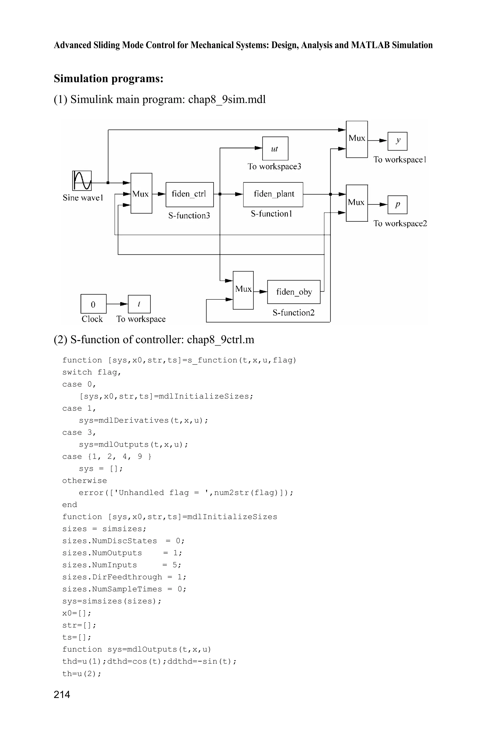
![8 Sliding Mode Control Based on Observer
211
2
ˆˆ ˆ( )d au k bZ Z T T (8.58)
where ˆd is the estimation of d, and ˆZ is the estimation of ,T 1 0,k ! 2 0k ! [9]
.
Select the Lyapunov function as
2 2
1
1
1 1
2 2
V d
k
Z (8.59)
where ˆ,d d d ˆ.Z T Z
Therefore, we have
1
1 1
1 1 ˆ ˆ( ) ( )V dd d d d
k k
ZZ Z T Z
From Eqs. (8.57) and (8.58), we have:
1 2
1 1
1 2
1 1
2
1
2
2 2
1 1
1 1 ˆ ˆ ˆ( ( ( ) ))
1 1 ˆˆ ˆ( ) ( ( ( ) ))
1 ˆˆ ˆ( ) ( ( ))
1 1
( ) 0
V dd dd d au k b
k k
dd dk b au d d au k b
k k
dd d d d k
k
dd d d k dd k
k k
Z T Z T T
Z T Z T Z T T
Z T Z Z T
Z Z Z Z
Suppose the disturbance d be a slow time-varying signal, and d is bounded.
When 1k is relative large, we can get
1
1
0.d
k
| At the same time, 2k is also
relative large, we can get:
2
1 2
1
1
0V dd k
k
Z (8.60)
The disturbance d can be estimated by the designed disturbance observer, and
the compensation will be realized in the feedback control.
8.8.3 Sliding Mode Controller Design
For system (8.56), let desired position input be d ,T and d .e T T The sliding
variable is selected as
s = e+ce (8.61)](https://image.slidesharecdn.com/advancedslidingmodecontrolformechanicalsystems-130611121131-phpapp01/75/Advanced-sliding-mode-control-for-mechanical-systems-228-2048.jpg)
![Advanced Sliding Mode Control for Mechanical Systems: Design, Analysis and MATLAB Simulation
212
where 0.c ! Therefore,
d ds e +ce ce b au d ceT T T T
The controller is adopted as
d
1 ˆ[ sgn( )]u b ce d s
a
T T K (8.62)
where ˆ,d d d | |.dK
Select the Lyapunov function as
2
2
1
2
V s
Therefore, we have
2 d
d d
( )
ˆ( ( sgn( )) )
ˆ( sgn( )) | | 0
V ss s b au d ce
s b b ce d s d ce
s d d s ds s
T T
T T T T K
K K
(8.63)
The Lyapunov function of the whole closed system can be described as
2 2 2
1 2
1
1 1 1
2 2 2
V V V d s
k
Z
From Eqs. (8.60) and (8.63), we can get 0.V
In order to restrain the chattering phenomenon, the saturated function sat( )s
is adopted instead of sgn( )s in Eq. (8.62),
1,
sat( ) , | | , 1/
1,
s
s ks s k
s
'
' '
'
!
°
®
° ¯
(8.64)
where ' is the “boundary layer”.
The nature of saturated function is: Out of the boundary layer, switch control
is selected, in the boundary layer, the usual feedback control is adopted.
Therefore, the chattering phenomenon can be restrained thoroughly.
8.8.4 Simulation Example
The kinetic equation of system is given as follow:
b au dT T](https://image.slidesharecdn.com/advancedslidingmodecontrolformechanicalsystems-130611121131-phpapp01/75/Advanced-sliding-mode-control-for-mechanical-systems-229-2048.jpg)
![Advanced Sliding Mode Control for Mechanical Systems: Design, Analysis and MATLAB Simulation
214
Simulation programs:
(1) Simulink main program: chap8_9sim.mdl
(2) S-function of controller: chap8_9ctrl.m
function [sys,x0,str,ts]=s_function(t,x,u,flag)
switch flag,
case 0,
[sys,x0,str,ts]=mdlInitializeSizes;
case 1,
sys=mdlDerivatives(t,x,u);
case 3,
sys=mdlOutputs(t,x,u);
case {1, 2, 4, 9 }
sys = [];
otherwise
error(['Unhandled flag = ',num2str(flag)]);
end
function [sys,x0,str,ts]=mdlInitializeSizes
sizes = simsizes;
sizes.NumDiscStates = 0;
sizes.NumOutputs = 1;
sizes.NumInputs = 5;
sizes.DirFeedthrough = 1;
sizes.NumSampleTimes = 0;
sys=simsizes(sizes);
x0=[];
str=[];
ts=[];
function sys=mdlOutputs(t,x,u)
thd=u(1);dthd=cos(t);ddthd=-sin(t);
th=u(2);](https://image.slidesharecdn.com/advancedslidingmodecontrolformechanicalsystems-130611121131-phpapp01/75/Advanced-sliding-mode-control-for-mechanical-systems-231-2048.jpg)
![8 Sliding Mode Control Based on Observer
215
dth=u(3);
dp=u(5);
b=0.15;a=5;
e=thd-th;
de=dthd-dth;
c=15;
s=c*e+de;
xite=5.0;
M=2;
if M==1
ut=1/a*(ddthd+b*dth+c*de+dp+xite*sign(s));
elseif M==2 %Saturated function
delta=0.10;
kk=1/delta;
if abs(s)delta
sats=sign(s);
else
sats=kk*s;
end
ut=1/a*(ddthd+b*dth+c*de+dp+xite*sign(s));
end
sys(1)=ut;
(3) Observer S-function: chap8_9obv.m
function [sys,x0,str,ts]=s_function(t,x,u,flag)
switch flag,
case 0,
[sys,x0,str,ts]=mdlInitializeSizes;
case 1,
sys=mdlDerivatives(t,x,u);
case 3,
sys=mdlOutputs(t,x,u);
case {2, 4, 9 }
sys = [];
otherwise
error(['Unhandled flag = ',num2str(flag)]);
end
function [sys,x0,str,ts]=mdlInitializeSizes
sizes = simsizes;
sizes.NumContStates = 2;
sizes.NumDiscStates = 0;
sizes.NumOutputs = 1;
sizes.NumInputs = 4;
sizes.DirFeedthrough = 0;
sizes.NumSampleTimes = 0;
sys=simsizes(sizes);
x0=[0;0];
str=[];](https://image.slidesharecdn.com/advancedslidingmodecontrolformechanicalsystems-130611121131-phpapp01/75/Advanced-sliding-mode-control-for-mechanical-systems-232-2048.jpg)
![Advanced Sliding Mode Control for Mechanical Systems: Design, Analysis and MATLAB Simulation
216
ts=[];
function sys=mdlDerivatives(t,x,u)
ut=u(1);
dth=u(3);
k1=5000;
k2=500;
a=5;b=0.15;
sys(1)=k1*(x(2)-dth);
sys(2)=-x(1)+a*ut-k2*(x(2)-dth)-b*dth;
function sys=mdlOutputs(t,x,u)
sys(1)=x(1); %d estimate
(4) S-function of the plant: chap8_9plant.m
function [sys,x0,str,ts]=s_function(t,x,u,flag)
switch flag,
case 0,
[sys,x0,str,ts]=mdlInitializeSizes;
case 1,
sys=mdlDerivatives(t,x,u);
case 3,
sys=mdlOutputs(t,x,u);
case {2, 4, 9 }
sys = [];
otherwise
error(['Unhandled flag = ',num2str(flag)]);
end
function [sys,x0,str,ts]=mdlInitializeSizes
sizes = simsizes;
sizes.NumContStates = 2;
sizes.NumDiscStates = 0;
sizes.NumOutputs = 3;
sizes.NumInputs = 1;
sizes.DirFeedthrough = 0;
sizes.NumSampleTimes = 0;
sys=simsizes(sizes);
x0=[0;0];
str=[];
ts=[];
function sys=mdlDerivatives(t,x,u)
ut=u(1);
b=0.15;
a=5;
d=100*sin(0.5*t);
ddth=-b*x(2)+a*ut-d;
sys(1)=x(2);](https://image.slidesharecdn.com/advancedslidingmodecontrolformechanicalsystems-130611121131-phpapp01/75/Advanced-sliding-mode-control-for-mechanical-systems-233-2048.jpg)
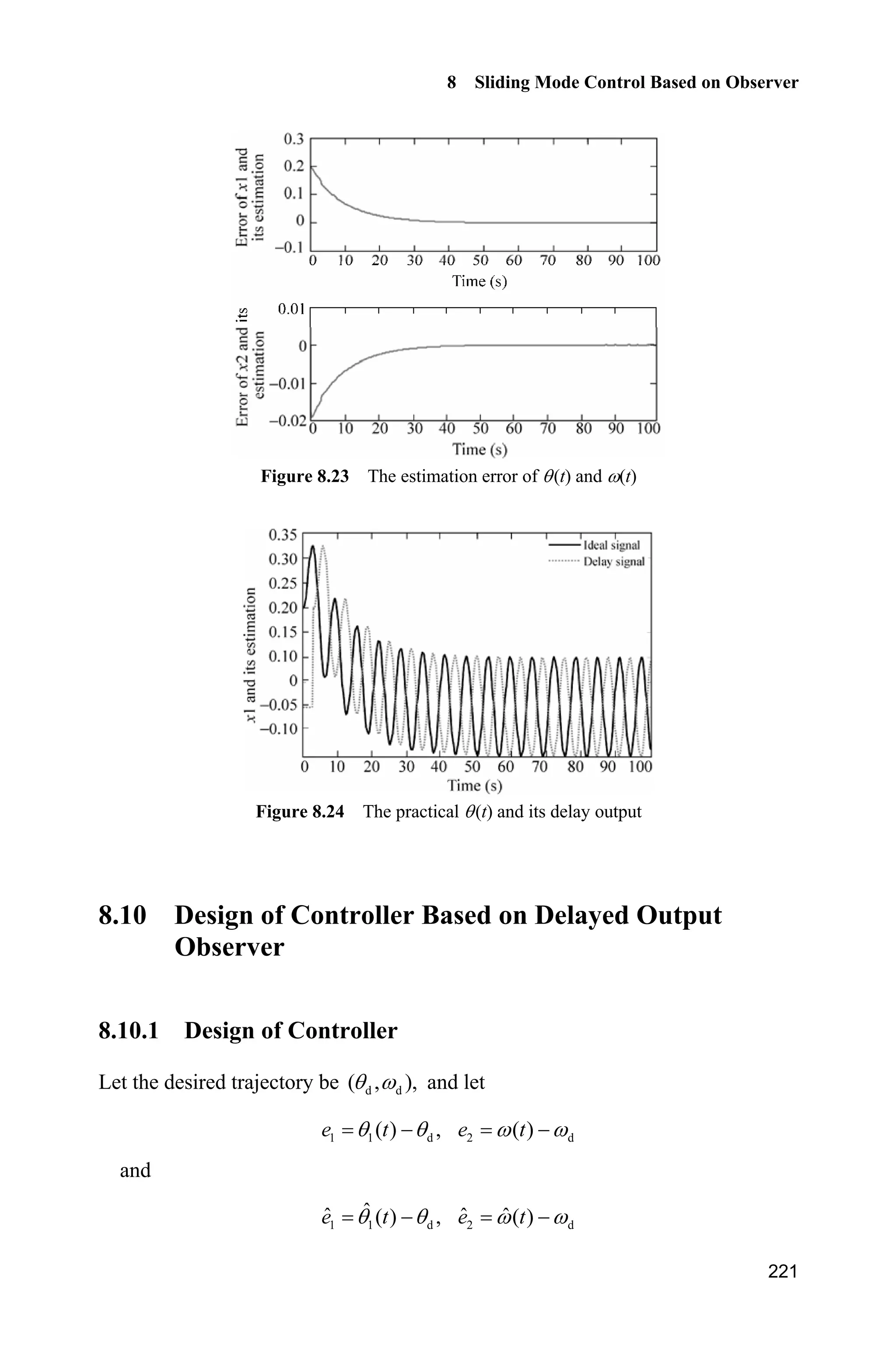
![Advanced Sliding Mode Control for Mechanical Systems: Design, Analysis and MATLAB Simulation
218
where T (t) denote angle at time t; u are the input signal, ( ) ( ).y t tT
Denote:
( ) [ ( ) ( )]T Z 7
t t tz
The goal is to observe that
ˆ ˆ( ) ( ), ( ) ( )t t t tT T Z Zo o as .t o f
where ' is the time delay brought from measurement delay.
8.9.2 Delayed Output Observer Design
We rewrite system (8.65) as:
( ) ( ) ( )t z t u tz A H (8.67)
where A is a Hurwitz matrix, and
0 1
,
1 10
ª º
« » ¬ ¼
A
0
.
1
ª º
« »
¬ ¼
H
The measurement outputs are:
( ) ( ) ( )y t t z tT ' ' C (8.68)
where (1 0).C
We design an observer[9]
for system (8.67) as follow:
ˆ ˆ ˆ( ) ( ) ( ) e [ ( ) ( )]t t u t y t t ''
A
z Az H K Cz (8.69)
ˆ ˆ ˆ( ) ( ) ( ) [ ( ) ( )]t t u t y t z t' ' ' ' z Az H K C (8.70)
where A must be Hurwitz, K is selected to make A KC Hurwitz, and
2 2 11
e
0 12!
I' '
' '
ª º
« »
¬ ¼
A
A A
Denote
1 2
ˆ ˆ( ) [ ( ) ( )] [ ( ) ( ) ( ) ( )]G G T T Z Z7 7
t t t t t t tį (8.71)
8.9.3 Delayed Output Observer Analysis
From Eq. (8.67), we have](https://image.slidesharecdn.com/advancedslidingmodecontrolformechanicalsystems-130611121131-phpapp01/75/Advanced-sliding-mode-control-for-mechanical-systems-235-2048.jpg)
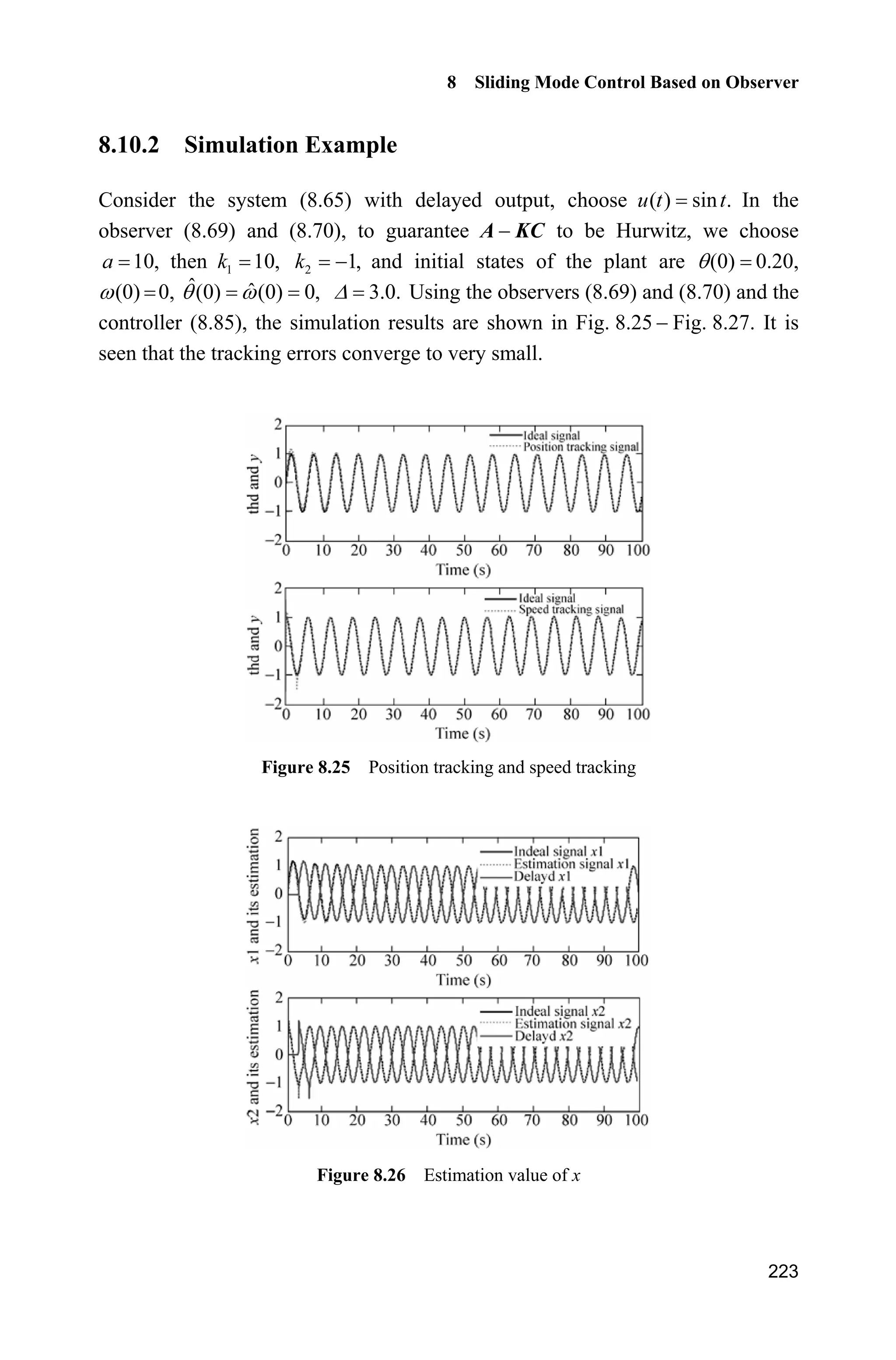
![0
0|| ( ) || || ( ) || e
t t
t l t
O
G ' G '
(8.76)
Lemma 1[9]
: The observer (8.79) is equivalent to the following relations:](https://image.slidesharecdn.com/advancedslidingmodecontrolformechanicalsystems-130611121131-phpapp01/75/Advanced-sliding-mode-control-for-mechanical-systems-237-2048.jpg)
![ˆ ˆ( ) ( ) e ( )d ( ) e ( )
ˆ ˆ ˆ( ) ( ( ) e ( )) ( ) e ( )
ˆ ˆ ˆ( ) ( ) e ( ( ) ( ) ( ))
t A tA A
t
A A A
A
z t e z t A Hu Hu t Hu t
e z t A z t z t Hu t Hu t
Az t Hu t z t Az t Hu t
W' '
'
' ' '
'
' W W '
' ' '
' ' '
³
(8.78)
From there it follows, after rearranging the terms in Eq. (8.78), we get
ˆ ˆ ˆ( ) ( ) ( ) e ( ( ) ( ))A
z t Az t Hu t K y t Cz t'
' (8.79)
This concludes Lemma 1.
Theorem 3[9]
: For system (8.73) with Eq. (8.74), and the designed observers
(8.69) and (8.70), there exist positive constants O and l such that
0( )
0|| ( ) || || e |||| ( ) || e t tA
t l t O'
G G '
(8.80)
where ( )tG is defined in Eq. (8.76).
Proof: From Eq. (8.73), we have
( )
( ) e ( ) e ( )d
t
A A t
t
z t z t Hu' W
'
' W W
³ (8.81)](https://image.slidesharecdn.com/advancedslidingmodecontrolformechanicalsystems-130611121131-phpapp01/75/Advanced-sliding-mode-control-for-mechanical-systems-239-2048.jpg)
![Advanced Sliding Mode Control for Mechanical Systems: Design, Analysis and MATLAB Simulation
220
From Eq. (8.77) in lemma 1 and Eq. (8.81), we can get
( ) e ( )A
t t'
G G ' (8.82)
Therefore, from Eqs. (8.76) and (8.82), we have
0( )
0|| ( ) || || e |||| ( ) || || e |||| ( ) || e t tA A
t t l t O' '
G G ' G '
(8.83)
This concludes the proof.
8.9.4 Simulation Example
Consider the system (8.65) with delayed output, choose ( ) sin .u t t
We select K to make A KC Hurwitz. Since
1 1
22
10 1
[1 0]
1 101 10
k k
kk
ª º ª ºª º
« » « »« » ¬ ¼ ¬ ¼¬ ¼
A KC
according to | ( ) | 0,O I A KC we can get 1
2
1
0,
1 10
k
k
O
O
that is
2
1 2 1( 10) 1 10 0.k k kO O From 2
( ) 0aO and 0,a ! we can get
2 2
2 0,a aO O then we can choose 1 10 2 ,k a 2
2 11 10 .k k a
To guarantee A KC to be Hurwitz, we can choose 10,a then 1 10,k
2 1,k and initial states of the plant and the observers (8.69) and (8.70) are
T (0) 0.20, Z(0) 0, ˆ ˆ(0) (0) 0,T Z 3.0.' The simulation results are
shown in Fig. 8.22 Fig. 8.24. It is seen that the observer errors asymptotically
converge to zero.
Figure 8.22 The estimation of T(t) and Z(t)](https://image.slidesharecdn.com/advancedslidingmodecontrolformechanicalsystems-130611121131-phpapp01/75/Advanced-sliding-mode-control-for-mechanical-systems-240-2048.jpg)
![Advanced Sliding Mode Control for Mechanical Systems: Design, Analysis and MATLAB Simulation
224
Figure 8.27 Control input
Simulation programs:
1. Observer program
(1) Simulink main program: chap8_10sim.mdl
(2) S-function of observer: chap8_10obv.m
function [sys,x0,str,ts]=s_function(t,x,u,flag)
switch flag,
case 0,
[sys,x0,str,ts]=mdlInitializeSizes;
case 1,
sys=mdlDerivatives(t,x,u);
case 3,
sys=mdlOutputs(t,x,u);
case {2, 4, 9 }](https://image.slidesharecdn.com/advancedslidingmodecontrolformechanicalsystems-130611121131-phpapp01/75/Advanced-sliding-mode-control-for-mechanical-systems-244-2048.jpg)
![8 Sliding Mode Control Based on Observer
225
sys = [];
otherwise
error(['Unhandled flag = ',num2str(flag)]);
end
function [sys,x0,str,ts]=mdlInitializeSizes
sizes = simsizes;
sizes.NumContStates = 4;
sizes.NumDiscStates = 0;
sizes.NumOutputs = 4;
sizes.NumInputs = 3;
sizes.DirFeedthrough = 1;
sizes.NumSampleTimes = 1;
sys=simsizes(sizes);
x0=[0 0 0 0];
str=[];
ts=[-1 0];
function sys=mdlDerivatives(t,x,u)
tol=3.0;
th_tol=u(1);
y3p=th_tol;
ut=u(2);
ut_tol=u(3);
z3_tol=[x(3);x(4)];
thp_tol=x(3);
thp=x(1);wp=x(2);
%%%%%%%%%
A=[0 1;-1 -10];
C=[1 0];
H3=[0;1];
k1=1;k2=2;
k1=10;k2=-1;
K=[k1 k2]';
z3=[thp wp]';
%%%%%%%%%
E=[exp(-1*tol) 0;0 exp(-1*tol)];
dz3=A*z3+H3*ut+E*K*(y3p-C*z3_tol);
dz3_tol=A*z3_tol+H3*ut_tol+K*(y3p-C*z3_tol);
for i=1:2
sys(i)=dz3(i);](https://image.slidesharecdn.com/advancedslidingmodecontrolformechanicalsystems-130611121131-phpapp01/75/Advanced-sliding-mode-control-for-mechanical-systems-245-2048.jpg)
![Advanced Sliding Mode Control for Mechanical Systems: Design, Analysis and MATLAB Simulation
226
sys(i+2)=dz3_tol(i);
end
function sys=mdlOutputs(t,x,u)
thp=x(1);wp=x(2);
thp_tol=x(3);wp_tol=x(4);
sys(1)=thp;
sys(2)=wp;
sys(3)=thp_tol;
sys(4)=wp_tol;
(3) S-function of plant: chap8_10plant.m
function [sys,x0,str,ts]=s_function(t,x,u,flag)
switch flag,
case 0,
[sys,x0,str,ts]=mdlInitializeSizes;
case 1,
sys=mdlDerivatives(t,x,u);
case 3,
sys=mdlOutputs(t,x,u);
case {2, 4, 9 }
sys = [];
otherwise
error(['Unhandled flag = ',num2str(flag)]);
end
function [sys,x0,str,ts]=mdlInitializeSizes
sizes = simsizes;
sizes.NumContStates = 2;
sizes.NumDiscStates = 0;
sizes.NumOutputs = 2;
sizes.NumInputs =1;
sizes.DirFeedthrough = 1;
sizes.NumSampleTimes = 1;
sys=simsizes(sizes);
x0=[0.2 0];
str=[];
ts=[-1 0];
function sys=mdlDerivatives(t,x,u)
sys(1)=x(2);
sys(2)=-10*x(2)-x(1)+u(1);
function sys=mdlOutputs(t,x,u)
th=x(1);w=x(2);
sys(1)=th;
sys(2)=w;
(4) S-function of plot: chap8_10plot.m
close all;](https://image.slidesharecdn.com/advancedslidingmodecontrolformechanicalsystems-130611121131-phpapp01/75/Advanced-sliding-mode-control-for-mechanical-systems-246-2048.jpg)
![Advanced Sliding Mode Control for Mechanical Systems: Design, Analysis and MATLAB Simulation
228
(2) S-function of controller: chap8_11ctrl.m
function [sys,x0,str,ts]=s_function(t,x,u,flag)
switch flag,
case 0,
[sys,x0,str,ts]=mdlInitializeSizes;
case 3,
sys=mdlOutputs(t,x,u);
case {1,2, 4, 9 }
sys = [];
otherwise
error(['Unhandled flag = ',num2str(flag)]);
end
function [sys,x0,str,ts]=mdlInitializeSizes
sizes = simsizes;
sizes.NumContStates = 0;
sizes.NumDiscStates = 0;
sizes.NumOutputs = 1;
sizes.NumInputs = 6;
sizes.DirFeedthrough = 1;
sizes.NumSampleTimes = 1;
sys=simsizes(sizes);
x0=[];
str=[];
ts=[-1 0];
function sys=mdlOutputs(t,x,u)
tol=3;
thd=1*sin(t);
wd=1*cos(t);
ddthd=-sin(t);
k1=10;k2=-1;
nmn=15;
thp=u(2);
wp=u(3);
thp_tol=u(4);
th_tol=u(6);
e1p=thp-thd;
e2p=wp-wd;
sp=e2p+nmn*e1p;
l=3.0;
fai=0.05;
if sp/fai1
sat=1;
elseif abs(sp/fai)=1
sat=sp/fai;
elseif sp/fai-1](https://image.slidesharecdn.com/advancedslidingmodecontrolformechanicalsystems-130611121131-phpapp01/75/Advanced-sliding-mode-control-for-mechanical-systems-248-2048.jpg)
![8 Sliding Mode Control Based on Observer
229
sat=-1;
end
%ut=thp+10*wp-l*sign(sp)+wd-nmn*e2p-(nmn*(k1+k2*tol)+k2)*(th_tol-thp_tol);
ut=thp+10*wp-l*sat+wd-nmn*e2p-(nmn*(k1+k2*tol)+k2)*(th_tol-thp_tol);
sys(1)=ut;
(3) S-function of observer: chap8_11obv.m
function [sys,x0,str,ts]=s_function(t,x,u,flag)
switch flag,
case 0,
[sys,x0,str,ts]=mdlInitializeSizes;
case 1,
sys=mdlDerivatives(t,x,u);
case 3,
sys=mdlOutputs(t,x,u);
case {2, 4, 9 }
sys = [];
otherwise
error(['Unhandled flag = ',num2str(flag)]);
end
function [sys,x0,str,ts]=mdlInitializeSizes
sizes = simsizes;
sizes.NumContStates = 4;
sizes.NumDiscStates = 0;
sizes.NumOutputs = 4;
sizes.NumInputs = 3;
sizes.DirFeedthrough = 1;
sizes.NumSampleTimes = 1;
sys=simsizes(sizes);
x0=[0 0 0 0];
str=[];
ts=[-1 0];
function sys=mdlDerivatives(t,x,u)
tol=3.0;
th_tol=u(1);
y3p=th_tol;
ut=u(2);
ut_tol=u(3);
z3_tol=[x(3);x(4)];
thp_tol=x(3);
thp=x(1);wp=x(2);
%%%%%%%%%
A=[0 1;-1 -10];
C=[1 0];](https://image.slidesharecdn.com/advancedslidingmodecontrolformechanicalsystems-130611121131-phpapp01/75/Advanced-sliding-mode-control-for-mechanical-systems-249-2048.jpg)
![Advanced Sliding Mode Control for Mechanical Systems: Design, Analysis and MATLAB Simulation
230
H3=[0;1];
k1=10;k2=-1;
K=[k1 k2]';
z3=[thp wp]';
%%%%%%%%%
E=[exp(-1*tol) 0;0 exp(-1*tol)];
dz3=A*z3+H3*ut+E*K*(y3p-C*z3_tol);
dz3_tol=A*z3_tol+H3*ut_tol+K*(y3p-C*z3_tol);
for i=1:2
sys(i)=dz3(i);
sys(i+2)=dz3_tol(i);
end
function sys=mdlOutputs(t,x,u)
thp=x(1);wp=x(2);
thp_tol=x(3);wp_tol=x(4);
sys(1)=thp;
sys(2)=wp;
sys(3)=thp_tol;
sys(4)=wp_tol;
(4) S-function of plant: chap8_11plant.m
function [sys,x0,str,ts]=s_function(t,x,u,flag)
switch flag,
case 0,
[sys,x0,str,ts]=mdlInitializeSizes;
case 1,
sys=mdlDerivatives(t,x,u);
case 3,
sys=mdlOutputs(t,x,u);
case {2, 4, 9 }
sys = [];
otherwise
error(['Unhandled flag = ',num2str(flag)]);
end
function [sys,x0,str,ts]=mdlInitializeSizes
sizes = simsizes;
sizes.NumContStates = 2;
sizes.NumDiscStates = 0;
sizes.NumOutputs = 2;
sizes.NumInputs =1;
sizes.DirFeedthrough = 1;
sizes.NumSampleTimes = 1;
sys=simsizes(sizes);
x0=[0.2 0];](https://image.slidesharecdn.com/advancedslidingmodecontrolformechanicalsystems-130611121131-phpapp01/75/Advanced-sliding-mode-control-for-mechanical-systems-250-2048.jpg)
![8 Sliding Mode Control Based on Observer
231
str=[];
ts=[-1 0];
function sys=mdlDerivatives(t,x,u)
sys(1)=x(2);
sys(2)=-10*x(2)-x(1)+u(1);
function sys=mdlOutputs(t,x,u)
th=x(1);w=x(2);
sys(1)=th;
sys(2)=w;
(5) S-function of plot: chap8_11plot.m
close all;
figure(1);
subplot(211);
plot(t,y(:,1),'k',t,y(:,2),'r:','linewidth',2);
xlabel('time(s)');ylabel('thd and y');
legend('ideal signal','position tracking signal');
subplot(212);
plot(t,cos(t),'k',t,y(:,3),'r:','linewidth',2);
xlabel('time(s)');ylabel('thd and y');
legend('ideal signal','speed tracking signal');
figure(2);
subplot(211);
plot(t,y1(:,1),'k',t,y1(:,3),'r:',t,y1(:,5),'b','linewidth',2);
xlabel('time(s)');ylabel('x1 and its estimation');
legend('ideal signal x1','estimation signal x1','delayed x1');
subplot(212);
plot(t,y1(:,2),'k',t,y1(:,4),'r:',t,y1(:,6),'b','linewidth',2);
xlabel('time(s)');ylabel('x2 and its estimation');
legend('ideal signal x2','estimation signal x2','delayed x2');
figure(3);
plot(t,ut(:,1),'k','linewidth',2);
xlabel('time(s)');ylabel('Control input');
References
[1] Kahlil HK. Nonlinear Systems, 3nd ed. Englewood Cliffs, NJ: Prentice-Hall, 2002
[2] Khalil HK. High-gain observers in nonlinear feedback control, Int. Conf. on Control,
Automation and Systems, Seoul, Korea, 2008
[3] Wang XH, Chen ZQ, Yuan ZZ. Output tracking based on extended observer for nonlinear
uncertain systems, Control and Decision, 2004, 19(10): 1113 1116 (In Chinese)](https://image.slidesharecdn.com/advancedslidingmodecontrolformechanicalsystems-130611121131-phpapp01/75/Advanced-sliding-mode-control-for-mechanical-systems-251-2048.jpg)
![Advanced Sliding Mode Control for Mechanical Systems: Design, Analysis and MATLAB Simulation
232
[4] Khalil HK. Nonlinear Systems, Prentice Hall, Upper Saddle River, New Jersey, 3rd edition,
2002
[5] Wang XH and Liu JK. Differentiator Design and Application-Filtering and Differentiating
for Signals (In Chinese)
[6] Ahrens JH, Khalil HK. High-gain observers in the presence of measurement noise: A
switched-gain approach, Automatica, 2009, 45: 936 943
[7] Slotine JJ. and Li WP. Applied nonlinear control. Prentice-Hall, 1991
[8] Atsuo K, Hiroshi I, Kiyoshi S. Chattering reduction of disturbance observer based sliding
mode control. IEEE Transactions on Industry Applications, 1994, 30(2): 456 461
[9] Wang XH, Liu JK, Cai KY. Tracking control for a velocity-sensorless VTOL aircraft with
delayed outputs, Automatica, 2009, 45: 2876 2882](https://image.slidesharecdn.com/advancedslidingmodecontrolformechanicalsystems-130611121131-phpapp01/75/Advanced-sliding-mode-control-for-mechanical-systems-252-2048.jpg)
![9 Fuzzy Sliding Mode Control
Jinkun Liu
Beijing University of Aeronautics and Astronautics
P.R.China
E-mail: ljk@buaa.edu.cn
Xinhua Wang
National University of Singapore
Singapore
E-mail: wangxinhua04@gmail.com
Abstract This chapter introduces four kinds of fuzzy sliding mode controllers
design, including fuzzy sliding mode control based on equivalent control,
sliding mode control based on fuzzy switch-gain regulation, sliding mode
control based on fuzzy system approximation and adaptive fuzzy control based
on fuzzy compensation for manipulator.
Keywords fuzzy sliding mode control, equivalent control, fuzzy switch-gain,
fuzzy system approximation, adaptive fuzzy control
Section 9.1 deals with the control system that comprises a logic fuzzy control
design and an equivalent control. We introduce a fuzzy sliding mode control based
on the equivalent control scheme for a class of nonlinear systems. The sliding
mode control law in the existing equivalent sliding mode control system is directly
substituted by a fuzzy logic controller. Hence, a control input without chattering
is obtained in the systems with uncertainties. The chattering phenomenon in the
sliding mode control is attenuated.
A chattering-free fuzzy sliding-mode control strategy for uncertain systems is
introduced in section 9.2. The discontinuous switch gain in the traditional sliding-
mode control is replaced by a fuzzy logic control. Hence, a control input without
chattering is obtained in the systems with uncertainties. Based on the Lyapunov
stability theory, we address the design schemes of the fuzzy sliding-mode control
where the fuzzy control is designed by a set of linguistic rules and the control
input is chattering free.
Past research of the universal approximation theorem[1]
shows that any nonlinear
function over a compact set with arbitrary accuracy can be approximated by a
Advanced Sliding Mode Control for Mechanical Systems
© Tsinghua University Press, Beijing and Springer-Verlag Berlin Heidelberg 201
J. Liu et al.,
2](https://image.slidesharecdn.com/advancedslidingmodecontrolformechanicalsystems-130611121131-phpapp01/75/Advanced-sliding-mode-control-for-mechanical-systems-253-2048.jpg)
![Advanced Sliding Mode Control for Mechanical Systems: Design, Analysis and MATLAB Simulation
234
fuzzy system. There have been significant research efforts on the adaptive fuzzy
control for nonlinear systems[2]
. Section 9.3 and section 9.4 propose an adaptive
fuzzy sliding mode control algorithm for a class of continuous time unknown
nonlinear systems. The unknown nonlinearities are approximated by the fuzzy
system with a set of fuzzy IF-THEN rules whose parameters are adjusted on-line
according to some adaptive laws. This aids in controlling the output of the nonlinear
system to track a given trajectory. The Lyapunov synthesis approach is used to
develop an adaptive control algorithm which is based on the adaptive fuzzy model.
The chattering action is attenuated and robust performance can be ensured. The
stability analysis for the proposed control algorithm is provided.
9.1 Fuzzy Sliding Mode Control Based on Equivalent
Control
In section 6 of Chapter 1, the equivalent sliding mode control has been described.
The control law consists of an equivalent control equ and a switch control su .
System states are kept on the sliding surface by an equivalent control and system
states attain the sliding surface by a switch control. Using fuzzy rules, the fuzzy
system is established based on the equivalent control and the switch control.
The sliding mode control based on an equivalent control uses the switching-gain
switch control to reduce the chattering phenomenon and guarantee the Lyapunov
stability. The small switching-gain switch control is adopted when the magnitudes
of disturbances are small and the large switching-gain switch control is adopted
when magnitudes of disturbances are large. This function can be realized by fuzzy
system with fuzzy rules[3]
.
9.1.1 Design of Fuzzy Control
Consider the following system with disturbances and uncertainties:
( , ) ( , ) ( ) ( )x f x t g x t u t d t (9.1)
Let the tracking error be de x x , and the switch function be
s ce e (9.2)
According to the sliding mode control theory, a sliding mode controller consists
of equivalent sliding mode control and switch control. The control law is shown
as follows:
If ( )s t is N then P is P (9.3a)
If ( )s t is Z then P is Z (9.3b)](https://image.slidesharecdn.com/advancedslidingmodecontrolformechanicalsystems-130611121131-phpapp01/75/Advanced-sliding-mode-control-for-mechanical-systems-254-2048.jpg)
![9 Fuzzy Sliding Mode Control
235
If ( )s t is P then P is P (9.3c)
where the fuzzy sets Z, N and P denote “zero”, “negative”, and “positive”
respectively.
Fuzzy rule (9.3b) states that the fuzzy controller is the equivalent control equ when
the switch function is equal to zero. Also, fuzzy rules (9.3a) and (9.3c) state that
the fuzzy controller is the equivalent control equ + P u the switch control su when
switch function is not equal to zero.
The output of the fuzzy deduce system is membership P . Adopting reverse
fuzzification method, the fuzzy control is designed as:
eq su u uP ˜ (9.4)
When 1P , eq su u u . Therefore, the control law is the traditional equivalent
sliding mode control. When 1P z , the chattering phenomenon can be reduced by
the variant membership P .
9.1.2 Simulation Example
Consider the kinetic equation of a single-stage inverted pendulum as follows:
1 2
2 ( ) ( ) ( )
x x
x f g u d t
®
˜ ¯ x x
where
2
1 2 1 1 c
2
1 c
sin cos sin /( )
( )
(4/3 cos /( ))
g x mlx x x m m
f
l m x m m
x
1 c
2
1 c
cos /( )
( )
(4/3 cos /( ))
x m m
g
l m x m m
x
1 2 1[ ],x x xx and 2x are the roll angle and roll rate respectively, 2
9.8 m /sg ,
u is the control input, c 1kgm is the mass of the vehicle, 0.1kgm is the
mass of the pendulum, 0.5 ml is the length of one half of the pendulum.
Consider the disturbance ( )d t with the form of Gauss function in the following:
2
2
( )
( ) 5exp
2
i
i
t c
d t
b
§ ·
¨ ¸
© ¹
Let 0.50ib , 5.0ic and 0.15K . The upper bound of disturbance is D
max(| ( ) |) 5.15d t K . The disturbance ( )d t is shown in Fig. 9.1. The desired
position trajectory is d sinx t.](https://image.slidesharecdn.com/advancedslidingmodecontrolformechanicalsystems-130611121131-phpapp01/75/Advanced-sliding-mode-control-for-mechanical-systems-255-2048.jpg)
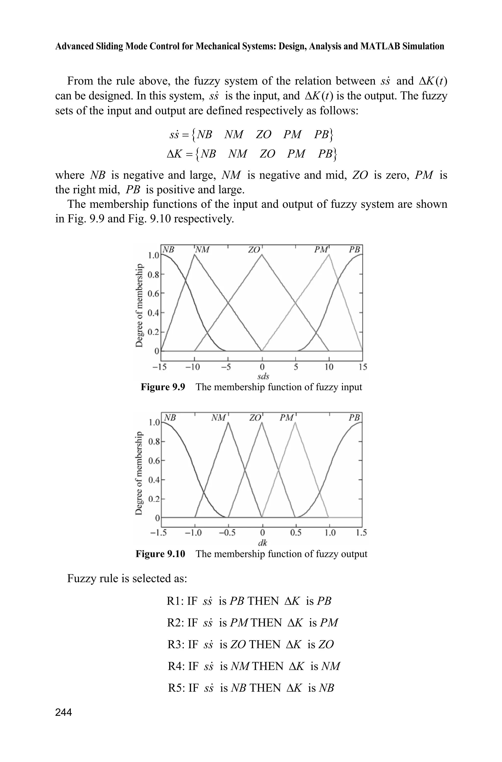
![Advanced Sliding Mode Control for Mechanical Systems: Design, Analysis and MATLAB Simulation
238
Figure 9.7 Control input ( 1)P z
Figure 9.8 Membership function ( ) ( 1)NZ sP P z
phenomenon can be reduced effectively when the fuzzy sliding mode control
based on an equivalent control is adopted.
Simulation programs:
(1) Fuzzy logic system program: chap9_1fuzz.m
close all
clear all;
a=newfis('fuzz_smc');
a=addvar(a,'input','s',1/25*[-25,25]);
a=addmf(a,'input',1,'N','trapmf',1/25*[-25,-25,-3,0]);
a=addmf(a,'input',1,'Z','trimf',1/25*[-3,0,3]);
a=addmf(a,'input',1,'P','trapmf',1/25*[0,3,25,25]);
% a=addvar(a,'output','Mu',20*[-5,5]);
% a=addmf(a,'output',1,'N','trapmf',20*[-5,-5,-3,0]);
% a=addmf(a,'output',1,'Z','trimf',20*[-3,0,3]);
% a=addmf(a,'output',1,'P','trapmf',20*[0,3,5,5]);](https://image.slidesharecdn.com/advancedslidingmodecontrolformechanicalsystems-130611121131-phpapp01/75/Advanced-sliding-mode-control-for-mechanical-systems-258-2048.jpg)
![9 Fuzzy Sliding Mode Control
239
a=addvar(a,'output','Mu',[-1,1]);
a=addmf(a,'output',1,'N','trapmf',[-1,-1,-0.5,0]);
a=addmf(a,'output',1,'Z','trapmf',[0,0.1,0.2,0.3]);
a=addmf(a,'output',1,'P','trapmf',[0,0.5,1,1]);
rulelist=[1 3 1 1;
2 2 1 1;
3 3 1 1];
a=addrule(a,rulelist);
showrule(a) %Show fuzzy rule base
a1=setfis(a,'DefuzzMethod','centroid'); %Defuzzy
a1=setfis(a,'DefuzzMethod','lom'); %Defuzzy
writefis(a1,'fsmc'); %Save fuzzy system as fsmc.fis
a2=readfis('fsmc');
ruleview(a2);
figure(1);
plotmf(a,'input',1);
figure(2);
plotmf(a,'output',1);
(2) Simulink main program: chap9_1sim.mdl
(3) S-function of controller: chap9_1ctrl.m
function [sys,x0,str,ts]=s_function(t,x,u,flag)
switch flag,
case 0,
[sys,x0,str,ts]=mdlInitializeSizes;
case 3,
sys=mdlOutputs(t,x,u);
case {2, 4, 9 }](https://image.slidesharecdn.com/advancedslidingmodecontrolformechanicalsystems-130611121131-phpapp01/75/Advanced-sliding-mode-control-for-mechanical-systems-259-2048.jpg)
![Advanced Sliding Mode Control for Mechanical Systems: Design, Analysis and MATLAB Simulation
240
sys = [];
otherwise
error(['Unhandled flag = ',num2str(flag)]);
end
function [sys,x0,str,ts]=mdlInitializeSizes
sizes = simsizes;
sizes.NumContStates = 0;
sizes.NumDiscStates = 0;
sizes.NumOutputs = 2;
sizes.NumInputs = 2;
sizes.DirFeedthrough = 1;
sizes.NumSampleTimes = 0;
sys=simsizes(sizes);
x0=[];
str=[];
ts=[];
function sys=mdlOutputs(t,x,u)
persistent a2
if t==0
a2=readfis('fsmc.fis');
end
xd=sin(t);
dxd=cos(t);
ddxd=-sin(t);
e=u(1);
de=u(2);
c=25;
s=c*e+de;
x1=xd-e;
x2=dxd-de;
g=9.8;mc=1.0;m=0.1;l=0.5;
S=l*(4/3-m*(cos(x1))^2/(mc+m));
fx=g*sin(x1)-m*l*x2^2*cos(x1)*sin(x1)/(mc+m);
fx=fx/S;
gx=cos(x1)/(mc+m);
gx=gx/S;
ueq=1/gx*(c*de+ddxd-fx);
D=5;
xite=D+0.15;
us=1/gx*xite*sign(s);
M=2;
if M==1 % Using conventional equavalent sliding mode control
Mu=1.0;
elseif M==2
Mu=evalfis([s],a2); % Using fuzzy equavalent sliding mode control](https://image.slidesharecdn.com/advancedslidingmodecontrolformechanicalsystems-130611121131-phpapp01/75/Advanced-sliding-mode-control-for-mechanical-systems-260-2048.jpg)
![9 Fuzzy Sliding Mode Control
241
end
ut=ueq+Mu*us;
sys(1)=ut;
sys(2)=Mu;
(4) S-function of the plant: chap9_1plant.m
function [sys,x0,str,ts]=s_function(t,x,u,flag)
switch flag,
case 0,
[sys,x0,str,ts]=mdlInitializeSizes;
case 1,
sys=mdlDerivatives(t,x,u);
case 3,
sys=mdlOutputs(t,x,u);
case {2, 4, 9 }
sys = [];
otherwise
error(['Unhandled flag = ',num2str(flag)]);
end
function [sys,x0,str,ts]=mdlInitializeSizes
sizes = simsizes;
sizes.NumContStates = 2;
sizes.NumDiscStates = 0;
sizes.NumOutputs = 2;
sizes.NumInputs = 1;
sizes.DirFeedthrough = 0;
sizes.NumSampleTimes = 0;
sys=simsizes(sizes);
x0=[pi/60 0];
str=[];
ts=[];
function sys=mdlDerivatives(t,x,u)
g=9.8;mc=1.0;m=0.1;l=0.5;
S=l*(4/3-m*(cos(x(1)))^2/(mc+m));
fx=g*sin(x(1))-m*l*x(2)^2*cos(x(1))*sin(x(1))/(mc+m);
fx=fx/S;
gx=cos(x(1))/(mc+m);
gx=gx/S;
%%%%%%%%%
bi=0.50;ci=5;
dt=5*exp(-(t-ci)^2/(2*bi^2)); %rbf_func.m
%%%%%%%%%
sys(1)=x(2);
sys(2)=fx+gx*u+dt;
function sys=mdlOutputs(t,x,u)
bi=0.50;ci=5;
dt=5*exp(-(t-ci)^2/(2*bi^2)); %rbf_func.m
sys(1)=x(1);
sys(2)=dt;](https://image.slidesharecdn.com/advancedslidingmodecontrolformechanicalsystems-130611121131-phpapp01/75/Advanced-sliding-mode-control-for-mechanical-systems-261-2048.jpg)
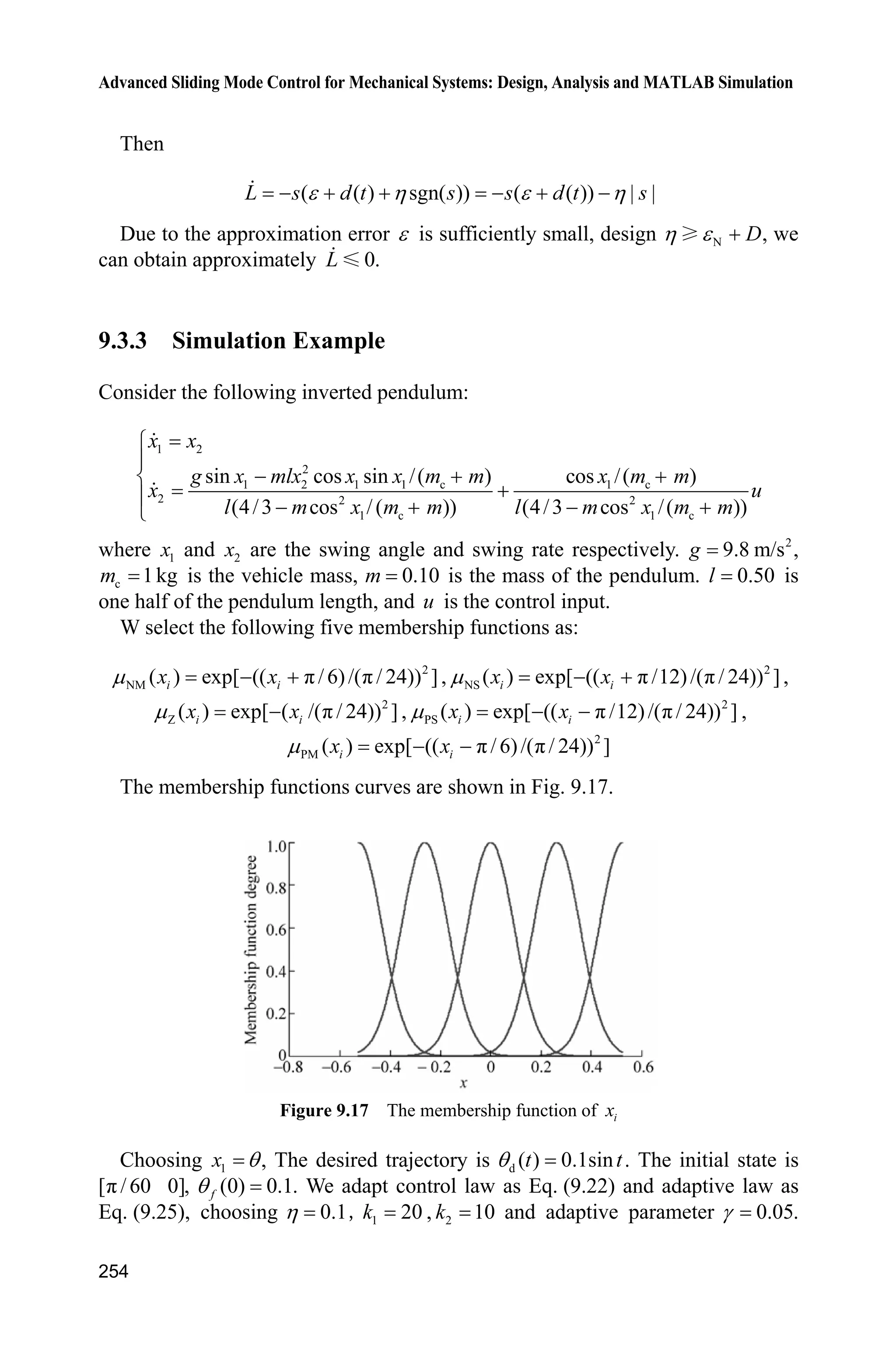
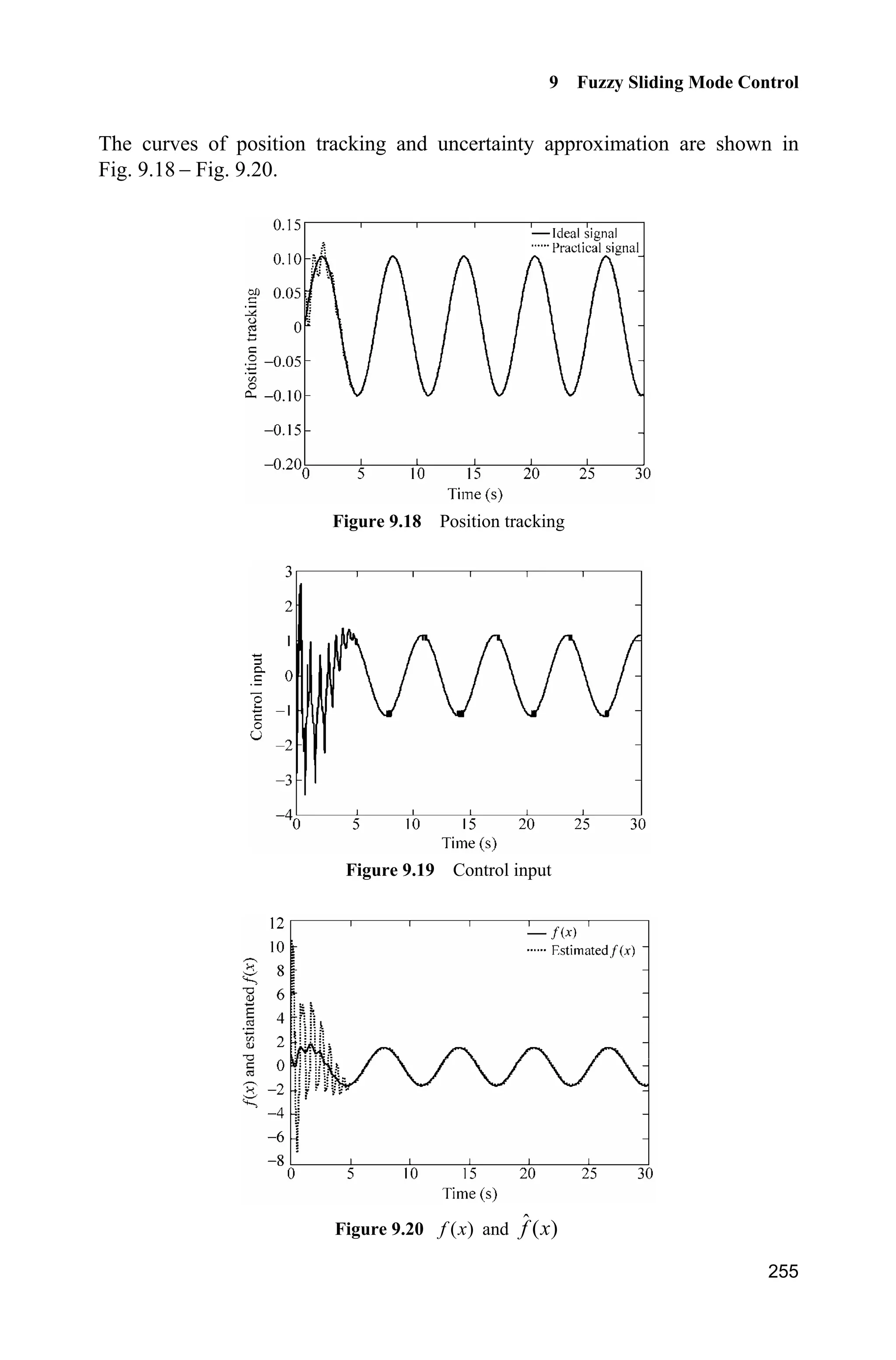
![Advanced Sliding Mode Control for Mechanical Systems: Design, Analysis and MATLAB Simulation
248
(2) S-function of controller: chap9_2ctrl.m
function [sys,x0,str,ts]=s_function(t,x,u,flag)
switch flag,
case 0,
[sys,x0,str,ts]=mdlInitializeSizes;
case 3,
sys=mdlOutputs(t,x,u);
case {2, 4, 9 }
sys = [];
otherwise
error(['Unhandled flag = ',num2str(flag)]);
end
function [sys,x0,str,ts]=mdlInitializeSizes
sizes = simsizes;
sizes.NumContStates = 0;
sizes.NumDiscStates = 0;
sizes.NumOutputs = 3;
sizes.NumInputs = 3;
sizes.DirFeedthrough = 1;
sizes.NumSampleTimes = 0;
sys=simsizes(sizes);
x0=[];
str=[];
ts=[];
function sys=mdlOutputs(t,x,u)
persistent s0
e=u(1);
de=u(2);
c=150;
thd=sin(2*pi*t);
dthd=2*pi*cos(2*pi*t);
ddthd=-(2*pi)^2*sin(2*pi*t);
x1=thd-e;
x2=dthd-de;
fx=-25*x2;b=133;
s=c*e+de;
D=200;xite=1.0;
M=2;
if M==1
K=D+xite;
elseif M==2 %Estimation for K with fuzzy
K=abs(u(3))+xite;
end](https://image.slidesharecdn.com/advancedslidingmodecontrolformechanicalsystems-130611121131-phpapp01/75/Advanced-sliding-mode-control-for-mechanical-systems-269-2048.jpg)
![9 Fuzzy Sliding Mode Control
249
ut=1/b*(-fx+ddthd+c*de+K*sign(s));
sys(1)=ut;
sys(2)=s;
sys(3)=K;
(3) S-function of the plant: chap9_2plant.m
function [sys,x0,str,ts]=s_function(t,x,u,flag)
switch flag,
case 0,
[sys,x0,str,ts]=mdlInitializeSizes;
case 1,
sys=mdlDerivatives(t,x,u);
case 3,
sys=mdlOutputs(t,x,u);
case {2, 4, 9 }
sys = [];
otherwise
error(['Unhandled flag = ',num2str(flag)]);
end
function [sys,x0,str,ts]=mdlInitializeSizes
sizes = simsizes;
sizes.NumContStates = 2;
sizes.NumDiscStates = 0;
sizes.NumOutputs = 2;
sizes.NumInputs = 1;
sizes.DirFeedthrough = 0;
sizes.NumSampleTimes = 0;
sys=simsizes(sizes);
x0=[0.15,0];
str=[];
ts=[];
function sys=mdlDerivatives(t,x,u)
%bi=0.05;ci=5;
bi=0.5;ci=5;
dt=200*exp(-(t-ci)^2/(2*bi^2)); %rbf_func.m
%dt=0;
sys(1)=x(2);
sys(2)=-25*x(2)+133*u+dt;
function sys=mdlOutputs(t,x,u)
%bi=0.05;ci=5;
bi=0.5;ci=5;
dt=200*exp(-(t-ci)^2/(2*bi^2)); %rbf_func.m
%dt=0;
sys(1)=x(1);
sys(2)=dt;](https://image.slidesharecdn.com/advancedslidingmodecontrolformechanicalsystems-130611121131-phpapp01/75/Advanced-sliding-mode-control-for-mechanical-systems-270-2048.jpg)
![Advanced Sliding Mode Control for Mechanical Systems: Design, Analysis and MATLAB Simulation
250
(4) S-function of fuzzy system: chap9_2rule.m
function [sys,x0,str,ts]=s_function(t,x,u,flag)
switch flag,
case 0,
[sys,x0,str,ts]=mdlInitializeSizes;
case 3,
sys=mdlOutputs(t,x,u);
case {2, 4, 9 }
sys = [];
otherwise
error(['Unhandled flag = ',num2str(flag)]);
end
function [sys,x0,str,ts]=mdlInitializeSizes
sizes = simsizes;
sizes.NumContStates = 0;
sizes.NumDiscStates = 0;
sizes.NumOutputs = 1;
sizes.NumInputs = 1;
sizes.DirFeedthrough = 1;
sizes.NumSampleTimes = 0;
sys=simsizes(sizes);
x0=[];
str=[];
ts=[];
function sys=mdlOutputs(t,x,u)
warning off;
persistent a1
if t==0
a1=readfis('smc_fuzz');
end
sys(1)=evalfis([u(1)],a1);
(5) Plot program: chap9_2plot.m
close all;
figure(1);
plot(t,y(:,1),'k',t,y(:,2),'r:','linewidth',2);
xlabel('time(s)');ylabel('Position tracking');
legend('Ideal position signal','tracking signal');
figure(2);
plot(t,E(:,1),'k',t,E(:,2),'r:','linewidth',2);
xlabel('time(s)');ylabel('E and estimated K');
legend('Ideal E','estimated E');
figure(3);
plot(t,ut(:,1),'k','linewidth',2);
xlabel('time(s)');ylabel('Control input');](https://image.slidesharecdn.com/advancedslidingmodecontrolformechanicalsystems-130611121131-phpapp01/75/Advanced-sliding-mode-control-for-mechanical-systems-271-2048.jpg)
![9 Fuzzy Sliding Mode Control
251
9.3 Sliding Mode Control Based on Fuzzy System
Approximation
9.3.1 Problem Statement
Consider a second-order nonlinear system as follows:
( , ) ( , ) ( )f g u d tT T T T T (9.12)
where f and g are all nonlinear functions, u R and is the input control, ( )d t is
the outer disturbance, and | ( ) |d t D.
Let the desired output be dT , and denote
de T T
Design the sliding mode function as
s = e+ce (9.13)
where 0c ! , then
d d ( )s e +ce ce f gu d t ceT T T (9.14)
If f and g are known, we can design control law as
d
1
[ sgn( )]u f ce s
g
T K (9.15)
Then Eq. (9.14) becomes
d d ( ) sgn( ) ( )s e +ce ce f gu d t ce s d tT T T K
Therefore, if DK , we have
| | ( ) 0ss s s d tK ˜
If ( )f x is unknown, we should estimate ( )f x by some algorithms. In the
following, we will simply recall fuzzy systems approximate uncertain item ( )f x .
9.3.2 Controller Design Based on Fuzzy System
9.3.2.1 Uncertainty Approximation Using Fuzzy System
If ( )f x is unknown, we can replace ( )f x with the fuzzy estimation ˆ( )f x to realize
feedback control[1]
. The universal approximation theorem is described as](https://image.slidesharecdn.com/advancedslidingmodecontrolformechanicalsystems-130611121131-phpapp01/75/Advanced-sliding-mode-control-for-mechanical-systems-272-2048.jpg)
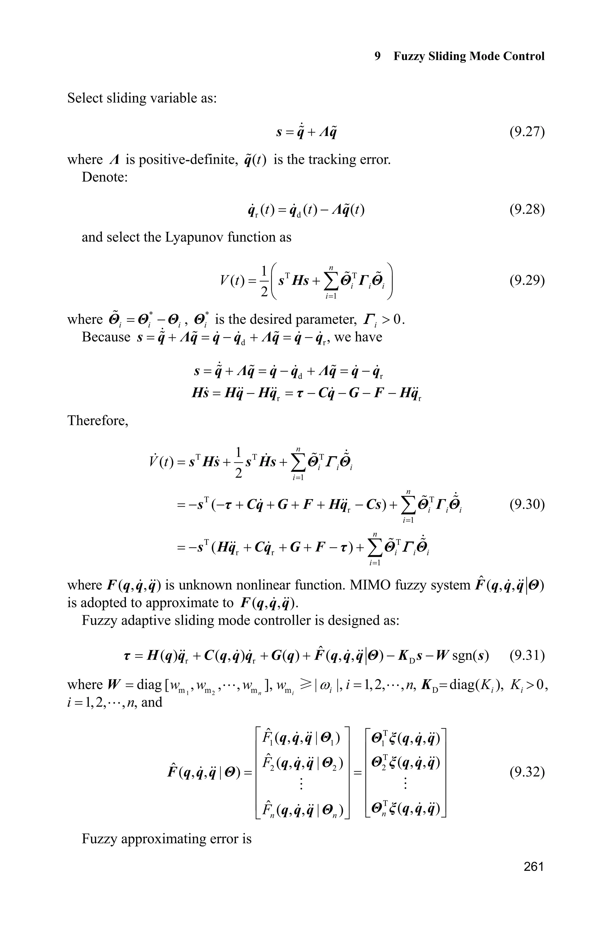
![9 Fuzzy Sliding Mode Control
253
The term f can be expressed as
*T
( )ff Hș ȟ x (9.20)
where x is the input signal of the fuzzy system, where ( )ȟ x is the fuzzy vector, H is
approximation error of fuzzy system, and NH H .
The fuzzy system is used to approximate f . The fuzzy system input is selected
as T
[ ]e ex , and the output of the fuzzy system is
Tˆ ˆ( | ) ( )f ff x ș ș ȟ x (9.21)
The control input Eq. (9.15) is written as
d
1 ˆ( sgn( ))u f ce s
g
T K (9.22)
Submitting Eqs. (9.22) to (9.14), we have
d d d
ˆ( ) ( sgn( )) ( )
ˆ sgn( ) ( ) ( ) sgn( )
s f gu d t ce f f ce s d t ce
f f s d t f d t s
T T T K
K K
(9.23)
Since
* T T Tˆ ˆ( ) ( ) ( )f f ff f f f H H ș ȟ x ș ȟ x ș ȟ x (9.24)
where * ˆ
f f fș ș ș .
Define the Lyapunov function as
2 T1 1
2 2
f fL s J ș ș
where 0J ! .
Derivative L, and from Eqs. (9.23) and (9.24), we have
T T
T T
T
ˆ( ( ) sgn( ))
ˆ( ( ) ( ) sgn( ))
ˆ( ( ) ) ( ( ) sgn( ))
f f f f
f f f
f f
L ss s f d t s
s d t s
s s d t s
J K J
H K J
J H K
ș ș ș ș
ș ȟ x ș ș
ș ȟ x ș
Let the adaptive rule be
1ˆ ( )f s
J
ș ȟ x (9.25)](https://image.slidesharecdn.com/advancedslidingmodecontrolformechanicalsystems-130611121131-phpapp01/75/Advanced-sliding-mode-control-for-mechanical-systems-275-2048.jpg)
![Advanced Sliding Mode Control for Mechanical Systems: Design, Analysis and MATLAB Simulation
254
Then
( ( ) sgn( )) ( ( )) | |L s d t s s d t sH K H K
Due to the approximation error H is sufficiently small, design N DK H , we
can obtain approximately 0L .
9.3.3 Simulation Example
Consider the following inverted pendulum:
1 2
2
1 2 1 1 c 1 c
2 2 2
1 c 1 c
sin cos sin /( ) cos /( )
(4/3 cos /( )) (4/3 cos /( ))
x x
g x mlx x x m m x m m
x u
l m x m m l m x m m
°
®
° ¯
where 1x and 2x are the swing angle and swing rate respectively. 2
9.8 m/sg ,
c 1kgm is the vehicle mass, 0.10m is the mass of the pendulum. 0.50l is
one half of the pendulum length, and u is the control input.
W select the following five membership functions as:
2
NM ( ) exp[ (( ʌ / 6)/(ʌ / 24)) ]i ix xP , 2
NS ( ) exp[ (( ʌ /12)/(ʌ / 24)) ]i ix xP ,
2
Z ( ) exp[ ( /(ʌ / 24)) ]i ix xP , 2
PS ( ) exp[ (( ʌ /12)/(ʌ / 24)) ]i ix xP ,
2
PM ( ) exp[ (( ʌ / 6)/(ʌ / 24)) ]i ix xP
The membership functions curves are shown in Fig. 9.17.
Figure 9.17 The membership function of ix
Choosing 1x T, The desired trajectory is d ( ) 0.1sint tT . The initial state is
[ʌ /60 0], (0) 0.1fT . We adapt control law as Eq. (9.22) and adaptive law as
Eq. (9.25), choosing 0.1K 1 20k , 2 10k and adaptive parameter 0.05J .](https://image.slidesharecdn.com/advancedslidingmodecontrolformechanicalsystems-130611121131-phpapp01/75/Advanced-sliding-mode-control-for-mechanical-systems-276-2048.jpg)
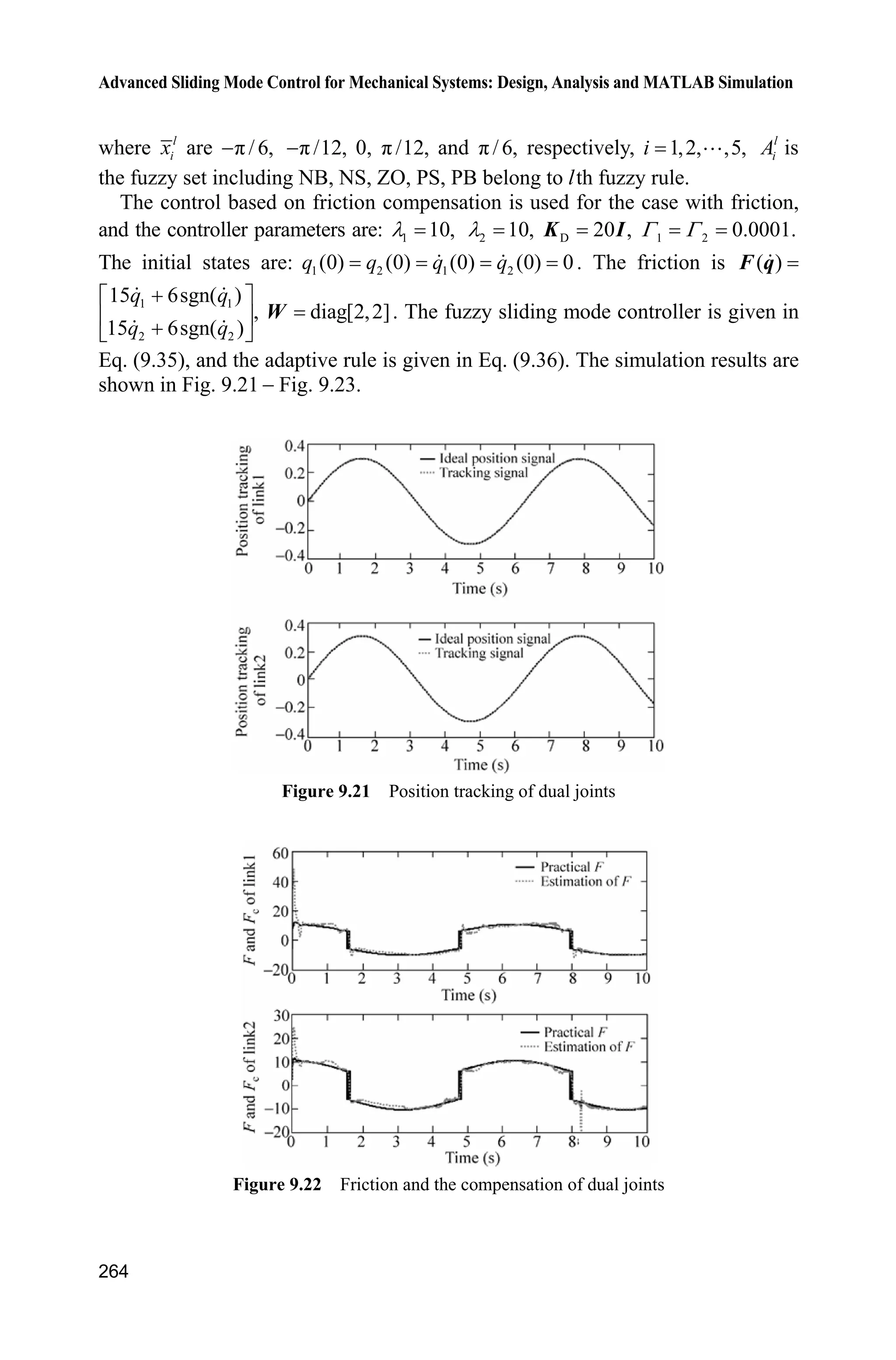
![Advanced Sliding Mode Control for Mechanical Systems: Design, Analysis and MATLAB Simulation
256
Simulation programs:
(1) Main Simulink program: chap9_3sim.mdl
(2) Control law program: chap9_3ctrl.m
function [sys,x0,str,ts] = spacemodel(t,x,u,flag)
switch flag,
case 0,
[sys,x0,str,ts]=mdlInitializeSizes;
case 1,
sys=mdlDerivatives(t,x,u);
case 3,
sys=mdlOutputs(t,x,u);
case {2,4,9}
sys=[];
otherwise
error(['Unhandled flag = ',num2str(flag)]);
end
function [sys,x0,str,ts]=mdlInitializeSizes
sizes = simsizes;
sizes.NumContStates = 25;
sizes.NumDiscStates = 0;
sizes.NumOutputs = 2;
sizes.NumInputs = 2;
sizes.DirFeedthrough = 1;
sizes.NumSampleTimes = 0;
sys = simsizes(sizes);
x0 = [zeros(25,1)];
str = [];
ts = [];
function sys=mdlDerivatives(t,x,u)
gama=0.005;
r=0.1*sin(t);
dr=0.1*cos(t);
ddr=-0.1*sin(t);](https://image.slidesharecdn.com/advancedslidingmodecontrolformechanicalsystems-130611121131-phpapp01/75/Advanced-sliding-mode-control-for-mechanical-systems-278-2048.jpg)
![9 Fuzzy Sliding Mode Control
257
e=u(1);
de=u(2);
n=25;
s=n*e+de;
x1=e;
x2=de;
for i=1:1:25
thtaf(i,1)=x(i);
end
%%%%%%%%%%%%%%%%%%%%%%%%%%%%%%%%
FS1=0;
for l1=1:1:5
gs1=-[(x1+pi/6-(l1-1)*pi/12)/(pi/24)]^2;
u1(l1)=exp(gs1);
end
for l2=1:1:5
gs2=-[(x2+pi/6-(l2-1)*pi/12)/(pi/24)]^2;
u2(l2)=exp(gs2);
end
for l1=1:1:5
for l2=1:1:5
FS2(5*(l1-1)+l2)=u1(l1)*u2(l2);
FS1=FS1+u1(l1)*u2(l2);
end
end
FS=FS2/FS1;
for i=1:1:25
sys(i)=-1/gama*s*FS(i);
end
function sys=mdlOutputs(t,x,u)
r=0.1*sin(t);
dr=0.1*cos(t);
ddr=-0.1*sin(t);
e=u(1);
de=u(2);
n=25;
s=n*e+de;
x1=e;
x2=de;
for i=1:1:25
thtaf(i,1)=x(i);
end](https://image.slidesharecdn.com/advancedslidingmodecontrolformechanicalsystems-130611121131-phpapp01/75/Advanced-sliding-mode-control-for-mechanical-systems-279-2048.jpg)
![Advanced Sliding Mode Control for Mechanical Systems: Design, Analysis and MATLAB Simulation
258
FS1=0;
for l1=1:1:5
gs1=-[(x1+pi/6-(l1-1)*pi/12)/(pi/24)]^2;
u1(l1)=exp(gs1);
end
for l2=1:1:5
gs2=-[(x2+pi/6-(l2-1)*pi/12)/(pi/24)]^2;
u2(l2)=exp(gs2);
end
for l1=1:1:5
for l2=1:1:5
FS2(5*(l1-1)+l2)=u1(l1)*u2(l2);
FS1=FS1+u1(l1)*u2(l2);
end
end
FS=FS2/FS1;
fxp=thtaf'*FS';
g=9.8;mc=1.0;m=0.1;l=0.5;
S=l*(4/3-m*(cos(x1))^2/(mc+m));
gx=cos(x1)/(mc+m);
gx=gx/S;
if t=1.0
xite=1.0;
else
xite=0.10;
end
ut=1/gx*(-fxp+ddr+n*de+xite*sign(s));
sys(1)=ut;
sys(2)=fxp;
(3) Membership function program: chap9_3mf.m
clear all;
close all;
L1=-pi/6;
L2=pi/6;
L=L2-L1;
T=L*1/1000;
x=L1:T:L2;
figure(1);
for i=1:1:5](https://image.slidesharecdn.com/advancedslidingmodecontrolformechanicalsystems-130611121131-phpapp01/75/Advanced-sliding-mode-control-for-mechanical-systems-280-2048.jpg)
![9 Fuzzy Sliding Mode Control
259
gs=-[(x+pi/6-(i-1)*pi/12)/(pi/24)].^2;
u=exp(gs);
hold on;
plot(x,u);
end
xlabel('x');ylabel('Membership function degree');
(4) Plant program: chap9_3plant.m
function [sys,x0,str,ts]=s_function(t,x,u,flag)
switch flag,
case 0,
[sys,x0,str,ts]=mdlInitializeSizes;
case 1,
sys=mdlDerivatives(t,x,u);
case 3,
sys=mdlOutputs(t,x,u);
case {2, 4, 9 }
sys = [];
otherwise
error(['Unhandled flag = ',num2str(flag)]);
end
function [sys,x0,str,ts]=mdlInitializeSizes
sizes = simsizes;
sizes.NumContStates = 2;
sizes.NumDiscStates = 0;
sizes.NumOutputs = 2;
sizes.NumInputs = 1;
sizes.DirFeedthrough = 0;
sizes.NumSampleTimes = 0;
sys=simsizes(sizes);
x0=[pi/60 0];
str=[];
ts=[];
function sys=mdlDerivatives(t,x,u)
g=9.8;mc=1.0;m=0.1;l=0.5;
S=l*(4/3-m*(cos(x(1)))^2/(mc+m));
fx=g*sin(x(1))-m*l*x(2)^2*cos(x(1))*sin(x(1))/(mc+m);
fx=fx/S;
gx=cos(x(1))/(mc+m);
gx=gx/S;
%%%%%%%%%
dt=0*10*sin(t);
%%%%%%%%%
sys(1)=x(2);
sys(2)=fx+gx*u+dt;
function sys=mdlOutputs(t,x,u)
g=9.8;
mc=1.0;](https://image.slidesharecdn.com/advancedslidingmodecontrolformechanicalsystems-130611121131-phpapp01/75/Advanced-sliding-mode-control-for-mechanical-systems-281-2048.jpg)
![9 Fuzzy Sliding Mode Control
261
Select sliding variable as:
s q ȁq (9.27)
where ȁ is positive-definite, ( )tq is the tracking error.
Denote:
r d( ) ( ) ( )t t tq q ȁq (9.28)
and select the Lyapunov function as
T T
1
1
( )
2
n
i i i
i
V t
§ ·
¨ ¸
© ¹
¦s Hs Ĭ ī Ĭ (9.29)
where *
i i iĬ Ĭ Ĭ , *
iĬ is the desired parameter, 0i !* .
Because d r s q ȁq q q ȁq q q , we have
d r s q ȁq q q ȁq q q
r r Hs Hq Hq IJ Cq G F Hq
Therefore,
T T T
1
T T
r
1
T T
r r
1
1
( )
2
( )
( )
n
i i i
i
n
i i i
i
n
i i i
i
V t
¦
¦
¦
s Hs s Hs Ĭ Ĭ
s IJ Cq G F Hq Cs Ĭ ī Ĭ
s Hq Cq G F IJ Ĭ Ĭ
*
*
(9.30)
where ( , , )F q q q is unknown nonlinear function. MIMO fuzzy system ˆ ( , , )F q q q Ĭ
is adopted to approximate to ( , , )F q q q .
Fuzzy adaptive sliding mode controller is designed as:
r r D
ˆ( ) ( , ) ( ) ( , , ) sgn( ) IJ H q q C q q q G q F q q q Ĭ K s W s (9.31)
where 1 2m m m mdiag [ , , , ], | |, 1,2, ,n i iw w w w i nZW , D diag( ),iKK 0iK ! ,
1,2, ,i n , and
T
1 1 1
T
22 2
T
ˆ ( , , | ) ( , , )
ˆ ( , , )( , , | )ˆ ( , , | )
ˆ ( , , )( , , | ) nn n
F
F
F
ª º ª º
« » « »
« » « »
« » « »
« » « »
« » « »¬ ¼¬ ¼
##
q q q Ĭ Ĭ ȟ q q q
Ĭ ȟ q q qq q q Ĭ
F q q q Ĭ
Ĭ ȟ q q qq q q Ĭ
(9.32)
Fuzzy approximating error is](https://image.slidesharecdn.com/advancedslidingmodecontrolformechanicalsystems-130611121131-phpapp01/75/Advanced-sliding-mode-control-for-mechanical-systems-283-2048.jpg)
![Advanced Sliding Mode Control for Mechanical Systems: Design, Analysis and MATLAB Simulation
262
*ˆ( , , ) ( , , | )Ȧ F q q q F q q q Ĭ (9.33)
From Eqs. (9.31) and (9.30), we have
T T
D
1
T *
* T
D
1
T T T
D
ˆ( ) ( ( , , ) ( , , | ) sgn( ))
ˆ ˆ( ( , , ) ( , , | ) ( , , | )
ˆ ( , , | ) sgn( ))
( ( , , ) sgn( ))
n
i i i
i
n
i i i
i
i i
i
V t
¦
¦
s F q q q F q q q Ĭ K s W s Ĭ Ĭ
s F q q q F q q q Ĭ F q q q Ĭ
F q q q Ĭ K s W s Ĭ Ĭ
s Ĭ ȟ q q q Ȧ K s W s Ĭ
*
*
*
1
T T T T
D
1
|| || ( ( , , ))
n
i
n
i i i i i
i
s
¦
¦
Ĭ
s K s s Ȧ W s Ĭ Ĭ Ĭ ȟ q q q*
where *
Ĭ Ĭ Ĭ, ( , , )ȟ q q q is the fuzzy system.
The adaptive rule is
1
( , , ), 1,2, ,i i is i n
Ĭ ȟ q q q * (9.34)
Therefore, we have
T T T
D D( ) || || 0V t s K s s Ȧ W s s K s
Suppose the joint number of manipulator is n, and if MIMO fuzzy system
ˆ ( , , | )F q q q Ĭ is adopted to approximate to ( , , )F q q q , then for each joint, the
number of input variables is 3. If k membership functions are designed for each
input variable, then the whole number of rules is 3n
k [4]
.
For instance, the joint number of the manipulator is 2, the number of input
variable is 3, there are 5 membership functions, then the whole rule number is
3 2 6
5 5 15625u
. The two many rules will bring out excessive computation. In order
to decrease the number of fuzzy rules, independent design should be adopted
with respect to ( , , , )tF q q q .
9.4.3 Control Based on Friction Compensation
When ( , , )F q q q only consists of rF , we can consider the case of fuzzy com-
pensation with respect to friction. Because the friction is relative to velocity, the
fuzzy system which approximates friction can be written as ˆ ( | )F q ș .
The method based on traditional fuzzy compensation, i.e., Eqs. (9.31) and (9.34),
is adopted to design the controller. The fuzzy adaptive sliding mode controller is
designed as:](https://image.slidesharecdn.com/advancedslidingmodecontrolformechanicalsystems-130611121131-phpapp01/75/Advanced-sliding-mode-control-for-mechanical-systems-284-2048.jpg)
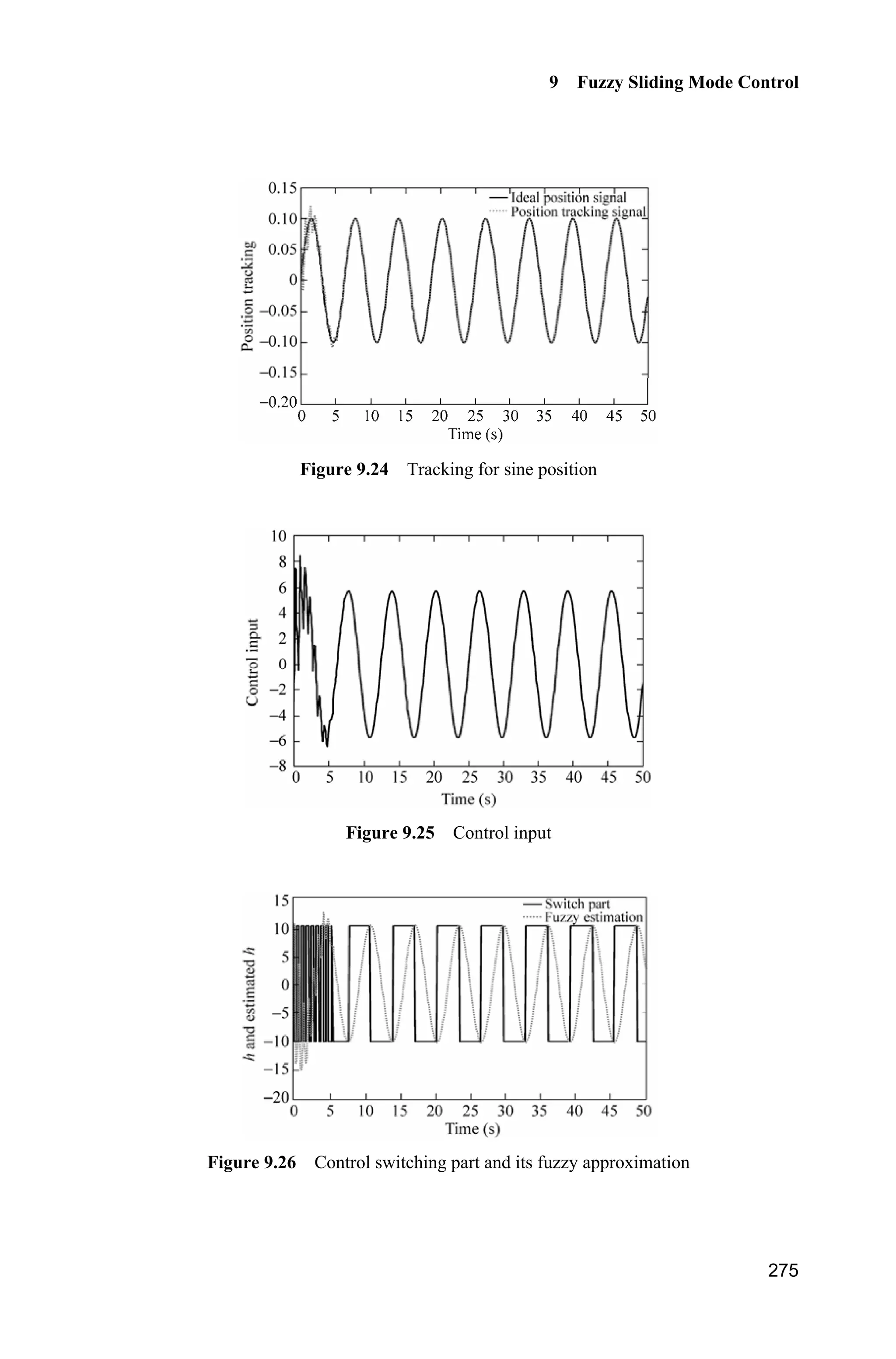
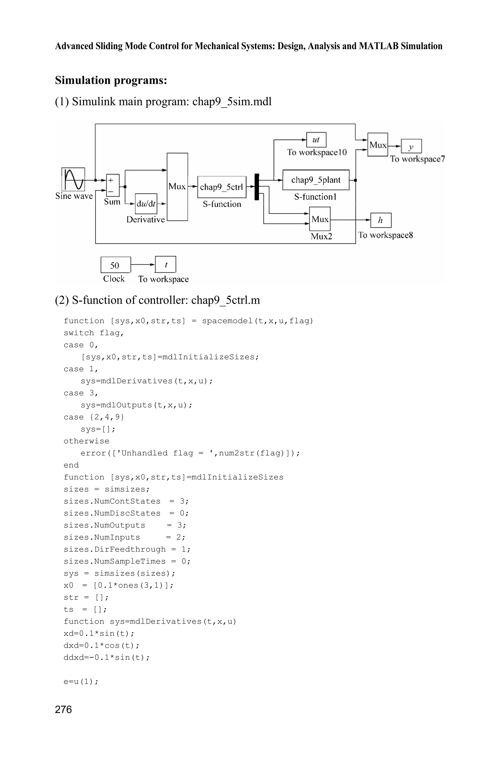
![11 2 12 2 12 2 2 12 2 1 21
221 2 22 2 12 2 1
1 1 2 1
22 1 2
0
( , , )
H q H q C q q C q q qq
qH q H q C q q
g q q g
F q q q
g q q g
W
W
§ · § ·§ ·
˜¨ ¸ ¨ ¸¨ ¸¨ ¸ ¨ ¸© ¹© ¹ © ¹
§ · § ·
¨ ¸ ¨ ¸¨ ¸ © ¹© ¹
where
2 2
11 2 1 2 1 2 2 2 1 2 2( ) ( ) 2 cos( )H q m m r m r m rr q
2
12 2 21 2 2 2 2 1 2 2( ) ( ) cos( )H q H q m r m rr q
2
22 2 2 2( )H q m r
12 2 2 1 2 2( ) sin( )C q m rr q
where 1m and 2m are the mass of link1 and link2, and 1r and 2r are the lengths
of link1 and link2.
Let T
1 2[ ] ,q qy T
1 2[ ] ,W WIJ T
1 1 2 2[ ] .q q q qx The parameters:
1 1m,r 2 0.8 m,r 1 1 kg,m 2 1.5 kg.m
The control object is to make the outputs 1,q 2q track the desired trajectories
d1 0.3siny t and d2 0.3siny t respectively. The membership function is defined
as:
2
( ) exp
ʌ / 24
l
i
l
i i
iA
x x
xP
§ ·§ ·
¨ ¸¨ ¸
¨ ¸© ¹© ¹](https://image.slidesharecdn.com/advancedslidingmodecontrolformechanicalsystems-130611121131-phpapp01/75/Advanced-sliding-mode-control-for-mechanical-systems-295-2048.jpg)
![Advanced Sliding Mode Control for Mechanical Systems: Design, Analysis and MATLAB Simulation
264
where l
ix are ʌ / 6, ʌ /12, 0, ʌ /12, and ʌ / 6, respectively, 1,2, ,5,i l
iA is
the fuzzy set including NB, NS, ZO, PS, PB belong to lth fuzzy rule.
The control based on friction compensation is used for the case with friction,
and the controller parameters are: 1 10,O 2 10,O D 20 ,K I 1 2 0.0001.* *
The initial states are: 1 2 1 2(0) (0) (0) (0) 0q q q q . The friction is ( )F q
1 1
2 2
15 6sgn( )
15 6sgn( )
ª º
« »
¬ ¼
q q
q q
, diag[2,2]W . The fuzzy sliding mode controller is given in
Eq. (9.35), and the adaptive rule is given in Eq. (9.36). The simulation results are
shown in Fig. 9.21 Fig. 9.23.
Figure 9.21 Position tracking of dual joints
Figure 9.22 Friction and the compensation of dual joints](https://image.slidesharecdn.com/advancedslidingmodecontrolformechanicalsystems-130611121131-phpapp01/75/Advanced-sliding-mode-control-for-mechanical-systems-296-2048.jpg)
![9 Fuzzy Sliding Mode Control
265
Figure 9.23 Control input of dual joints
Simulation program:
Control based on friction fuzzy compensation for manipulator
(1) Simulink main program: chap9_4sim.mdl
(2) S-function of controller: chap9_4ctrl.m
function [sys,x0,str,ts] = MIMO_Tong_s(t,x,u,flag)
switch flag,
case 0,
[sys,x0,str,ts]=mdlInitializeSizes;](https://image.slidesharecdn.com/advancedslidingmodecontrolformechanicalsystems-130611121131-phpapp01/75/Advanced-sliding-mode-control-for-mechanical-systems-297-2048.jpg)
![Advanced Sliding Mode Control for Mechanical Systems: Design, Analysis and MATLAB Simulation
266
case 1,
sys=mdlDerivatives(t,x,u);
case 3,
sys=mdlOutputs(t,x,u);
case {2,4,9}
sys=[];
otherwise
error(['Unhandled flag = ',num2str(flag)]);
end
function [sys,x0,str,ts]=mdlInitializeSizes
global nmn1 nmn2 Fai
nmn1=10;nmn2=10;
Fai=[nmn1 0;0 nmn2];
sizes = simsizes;
sizes.NumContStates = 10;
sizes.NumDiscStates = 0;
sizes.NumOutputs = 4;
sizes.NumInputs = 8;
sizes.DirFeedthrough = 1;
sizes.NumSampleTimes = 0;
sys = simsizes(sizes);
x0 = [0.1*ones(10,1)];
str = [];
ts = [];
function sys=mdlDerivatives(t,x,u)
global nmn1 nmn2 Fai
qd1=u(1);
qd2=u(2);
dqd1=0.3*cos(t);
dqd2=0.3*cos(t);
dqd=[dqd1 dqd2]';
ddqd1=-0.3*sin(t);
ddqd2=-0.3*sin(t);
ddqd=[ddqd1 ddqd2]';
q1=u(3);dq1=u(4);
q2=u(5);dq2=u(6);
%%%%%%%%%%%%%%%%%%%%%%%%%%%%%%%%%%%%%%%%%%%
fsd1=0;
for l1=1:1:5
gs1=-[(dq1+pi/6-(l1-1)*pi/12)/(pi/24)]^2;
u1(l1)=exp(gs1);
end
fsd2=0;
for l2=1:1:5
gs2=-[(dq2+pi/6-(l2-1)*pi/12)/(pi/24)]^2;
u2(l2)=exp(gs2);
end](https://image.slidesharecdn.com/advancedslidingmodecontrolformechanicalsystems-130611121131-phpapp01/75/Advanced-sliding-mode-control-for-mechanical-systems-298-2048.jpg)
![9 Fuzzy Sliding Mode Control
267
for l1=1:1:5
fsu1(l1)=u1(l1);
fsd1=fsd1+u1(l1);
end
for l2=1:1:5
fsu2(l2)=u2(l2);
fsd2=fsd2+u2(l2);
end
fs1=fsu1/(fsd1+0.001);
fs2=fsu2/(fsd2+0.001);
%%%%%%%%%%%%%%%%%%%%%%%%%%%%%%%%%%%%%%%%%%%
e1=q1-qd1;
e2=q2-qd2;
e=[e1 e2]';
de1=dq1-dqd1;
de2=dq2-dqd2;
de=[de1 de2]';
s=de+Fai*e;
Gama1=0.0001;Gama2=0.0001;
S1=-1/Gama1*s(1)*fs1;
S2=-1/Gama2*s(2)*fs2;
for i=1:1:5
sys(i)=S1(i);
end
for j=6:1:10
sys(j)=S2(j-5);
end
function sys=mdlOutputs(t,x,u)
global nmn1 nmn2 Fai
q1=u(3);dq1=u(4);
q2=u(5);dq2=u(6);
r1=1;r2=0.8;
m1=1;m2=1.5;
H11=(m1+m2)*r1^2+m2*r2^2+2*m2*r1*r2*cos(q2);
H22=m2*r2^2;
H21=m2*r2^2+m2*r1*r2*cos(q2);
H12=H21;
H=[H11 H12;H21 H22];
C12=m2*r1*sin(q2);
C=[-C12*dq2 -C12*(dq1+dq2);C12*q1 0];
g1=(m1+m2)*r1*cos(q2)+m2*r2*cos(q1+q2);
g2=m2*r2*cos(q1+q2);](https://image.slidesharecdn.com/advancedslidingmodecontrolformechanicalsystems-130611121131-phpapp01/75/Advanced-sliding-mode-control-for-mechanical-systems-299-2048.jpg)
![Advanced Sliding Mode Control for Mechanical Systems: Design, Analysis and MATLAB Simulation
268
G=[g1;g2];
qd1=u(1);
qd2=u(2);
dqd1=0.3*cos(t);
dqd2=0.3*cos(t);
dqd=[dqd1 dqd2]';
ddqd1=-0.3*sin(t);
ddqd2=-0.3*sin(t);
ddqd=[ddqd1 ddqd2]';
e1=q1-qd1;
e2=q2-qd2;
e=[e1 e2]';
de1=dq1-dqd1;
de2=dq2-dqd2;
de=[de1 de2]';
s=de+Fai*e;
dqr=dqd-Fai*e;
ddqr=ddqd-Fai*de;
for i=1:1:5
thta1(i,1)=x(i);
end
for i=1:1:5
thta2(i,1)=x(i+5);
end
fsd1=0;
for l1=1:1:5
gs1=-[(dq1+pi/6-(l1-1)*pi/12)/(pi/24)]^2;
u1(l1)=exp(gs1);
end
fsd2=0;
for l2=1:1:5
gs2=-[(dq2+pi/6-(l2-1)*pi/12)/(pi/24)]^2;
u2(l2)=exp(gs2);
end
for l1=1:1:5
fsu1(l1)=u1(l1);
fsd1=fsd1+u1(l1);
end
for l2=1:1:5
fsu2(l2)=u2(l2);
fsd2=fsd2+u2(l2);](https://image.slidesharecdn.com/advancedslidingmodecontrolformechanicalsystems-130611121131-phpapp01/75/Advanced-sliding-mode-control-for-mechanical-systems-300-2048.jpg)
![9 Fuzzy Sliding Mode Control
269
end
fs1=fsu1/(fsd1+0.001);
fs2=fsu2/(fsd2+0.001);
Fp(1)=thta1'*fs1';
Fp(2)=thta2'*fs2';
KD=20*eye(2);
W=[1.5 0;0 1.5];
tol=H*ddqr+C*dqr+G+1*Fp'-KD*s-W*sign(s); %(4.134)
sys(1)=tol(1);
sys(2)=tol(2);
sys(3)=Fp(1);
sys(4)=Fp(2);
(3) Membership function program: chap9_4mf.m
clear all;
close all;
L1=-pi/6;
L2=pi/6;
L=L2-L1;
T=L*1/1000;
x=L1:T:L2;
figure(1);
for i=1:1:5
gs=-[(x+pi/6-(i-1)*pi/12)/(pi/24)].^2;
u=exp(gs);
hold on;
plot(x,u);
end
xlabel('x');ylabel('Membership function degree');
(4) S-function of the plant: chap9_4plant.m
function [sys,x0,str,ts]=MIMO_Tong_plant(t,x,u,flag)
switch flag,
case 0,
[sys,x0,str,ts]=mdlInitializeSizes;
case 1,
sys=mdlDerivatives(t,x,u);
case 3,
sys=mdlOutputs(t,x,u);
case {2, 4, 9 }
sys = [];
otherwise](https://image.slidesharecdn.com/advancedslidingmodecontrolformechanicalsystems-130611121131-phpapp01/75/Advanced-sliding-mode-control-for-mechanical-systems-301-2048.jpg)
![Advanced Sliding Mode Control for Mechanical Systems: Design, Analysis and MATLAB Simulation
270
error(['Unhandled flag = ',num2str(flag)]);
end
function [sys,x0,str,ts]=mdlInitializeSizes
sizes = simsizes;
sizes.NumContStates = 4;
sizes.NumDiscStates = 0;
sizes.NumOutputs = 6;
sizes.NumInputs = 4;
sizes.DirFeedthrough = 0;
sizes.NumSampleTimes = 0;
sys=simsizes(sizes);
x0=[0 0 0 0];
str=[];
ts=[];
function sys=mdlDerivatives(t,x,u)
r1=1;r2=0.8;
m1=1;m2=1.5;
H11=(m1+m2)*r1^2+m2*r2^2+2*m2*r1*r2*cos(x(3));
H22=m2*r2^2;
H21=m2*r2^2+m2*r1*r2*cos(x(3));
H12=H21;
H=[H11 H12;H21 H22];
C12=m2*r1*sin(x(3));
C=[-C12*x(4) -C12*(x(2)+x(4));C12*x(1) 0];
g1=(m1+m2)*r1*cos(x(3))+m2*r2*cos(x(1)+x(3));
g2=m2*r2*cos(x(1)+x(3));
G=[g1;g2];
Fr=[15*x(2)+6*sign(x(2));15*x(4)+6*sign(x(4))];
tol=[u(1) u(2)]';
S=inv(H)*(tol-C*[x(2);x(4)]-G-Fr);
sys(1)=x(2);
sys(2)=S(1);
sys(3)=x(4);
sys(4)=S(2);
function sys=mdlOutputs(t,x,u)
Fr=[15*x(2)+6*sign(x(2));15*x(4)+6*sign(x(4))];
sys(1)=x(1);
sys(2)=x(2);
sys(3)=x(3);
sys(4)=x(4);
sys(5)=Fr(1);
sys(6)=Fr(2);](https://image.slidesharecdn.com/advancedslidingmodecontrolformechanicalsystems-130611121131-phpapp01/75/Advanced-sliding-mode-control-for-mechanical-systems-302-2048.jpg)
![9 Fuzzy Sliding Mode Control
271
(5) Plot program: chap9_4plot.m
close all;
figure(1);
subplot(211);
plot(t,yd1(:,1),'k',t,y(:,1),'r:','linewidth',2);
xlabel('time(s)');ylabel('Position tracking of link1');
legend('Ideal position signal','tracking signal');
subplot(212);
plot(t,yd2(:,1),'k',t,y(:,3),'r:','linewidth',2);
xlabel('time(s)');ylabel('Position tracking of link2');
legend('Ideal position signal','tracking signal');
figure(2);
subplot(211);
plot(t,y(:,5),'k',t,u(:,3),'r:','linewidth',2);
xlabel('time(s)');ylabel('F and Fc of link1');
legend('Practical F','Estimation of F');
subplot(212);
plot(t,y(:,6),'k',t,u(:,4),'r:','linewidth',2);
xlabel('time(s)');ylabel('F and Fc of link2');
legend('Practical F','Estimation of F');
figure(3);
subplot(211);
plot(t,u(:,1),'r','linewidth',2);
xlabel('time(s)');ylabel('Control input of Link1');
subplot(212);
plot(t,u(:,2),'r','linewidth',2);
xlabel('time(s)');ylabel('Control input of Link2');
9.5 Adaptive Sliding Mode Control Based on Switching
Fuzzy
Using the adaptive fuzzy control method, the switching item in the sliding mode
controller is approximated and the switching item is continued. Therefore, the
chattering phenomenon can be reduced sufficiently[5]
.
9.5.1 Plant Description
Considering the following n-order SISO nonlinear system:
1 2
2 3
( , ) ( , ) ( ) ( )n
x x
x x
x f t g t u t d t x x
#
(9.37)](https://image.slidesharecdn.com/advancedslidingmodecontrolformechanicalsystems-130611121131-phpapp01/75/Advanced-sliding-mode-control-for-mechanical-systems-303-2048.jpg)
![Advanced Sliding Mode Control for Mechanical Systems: Design, Analysis and MATLAB Simulation
272
1y x
where f and g are the known nonlinear function, n
x R , u R, y R, ( )d t
is the unknown disturbance, | ( ) | ,d t D ( , ) 0.g t !x
9.5.2 Design of Adaptive Fuzzy Sliding Mode Controller
The switching function is defined as
( 1) ( 1)
1 2 1( )n n
ns k e k e k e e k
e (9.38)
where ( 1) T
d [ ] ,
n
e e ee x x 1 2 1, , , nk k k is satisfied with Hurwitzian
stability condition.
The sliding mode controller is designed as
1
( ) ( )
d sw
1
1
( ) ( , )
( , )
n
i n
i
i
u t f t k e x u
g t
§ ·
¨ ¸
© ¹
¦x
x
(9.39)
where sw sgn( ),u sK .DK !
From Eqs. (9.37) and (9.38), we get](https://image.slidesharecdn.com/advancedslidingmodecontrolformechanicalsystems-130611121131-phpapp01/75/Advanced-sliding-mode-control-for-mechanical-systems-304-2048.jpg)
![1
( ) ( ) ( )
d
1
1
( )
d
1
( , ) ( , ) ( ) ( )
n
i n n
i
i
n
i n
i
i
s k e x x
k e f t g t u t d t x
¦
¦ x x
(9.40)
And from Eq. (9.39), we have
( ) sgn( )s d t sK
i.e.
( ) | | 0ss d t s sK (9.41)
When d is relative large, the switching item K in controller (9.39) is large. This
results in serious chattering phenomenon. Fuzzy system ˆh is used to approximate
sgn( ).sK Therefore, the switching signal is weakened and the chattering phenomenon
can be reduced.
Using product deduce, single-value fuzzy and center average fuzzy, the fuzzy
output is ˆ.h From Eq. (9.39), the controller is written as[5]
1
( ) ( )
d
1
1 ˆ( ) ( , ) ( )
( , )
n
i n
i
i
u t f t k e x h s
g t
§ ·
¨ ¸
© ¹
¦x
x
(9.42)](https://image.slidesharecdn.com/advancedslidingmodecontrolformechanicalsystems-130611121131-phpapp01/75/Advanced-sliding-mode-control-for-mechanical-systems-305-2048.jpg)
![9 Fuzzy Sliding Mode Control
273
T
h h
ˆ( | ) ( )h s sIT T (9.43)
where h
ˆ( | )h s T is the fuzzy output of the universal approximation Eq. (9.18),
( )sI is the fuzzy vector, vector T
hT varies according to the adaptive rule. The
ideal h
ˆ( | )h s T is
*
h
ˆ( | ) sgn( )h s sKT (9.44)
where .DK !
The adaptive rule is:
h ( )s sJT I (9.45)
where 0.J !
Proof:
The optimization parameter is defined as:
h h
*
h h
ˆarg min[sup | ( | ) sgn( ) |]h s s
:
K
T
T T (9.46)
where h: is the set of h .T
Therefore, we have
1
( ) ( ) ( )
d
1
1
( ) ( )
d
1
h
* *
h h h
T *
h h
( , ) ( , ) ( ) ( )
ˆ( | ) ( )
ˆ ˆ ˆ( | ) ( ) ( | ) ( | )
ˆ( ) ( ) ( | )
n
i n n
i
i
n
i n
i
i
s k e x x
k e f x t g x t u t d t x
h s d t
h s d t h s h s
s d t h sI
¦
¦
T
T T T
T T (9.47)
where *
h h h .T T T
The Lyapunov function is selected as
2 T
h h
1 1
2
V s
J
§ ·
¨ ¸
© ¹
T T (9.48)
Therefore,
T
h h
T * T
h h h h
1
1ˆ( ( ) ( ) ( | ))
V ss
s s d t h s
J
J
T T
T I T T T](https://image.slidesharecdn.com/advancedslidingmodecontrolformechanicalsystems-130611121131-phpapp01/75/Advanced-sliding-mode-control-for-mechanical-systems-306-2048.jpg)
![Advanced Sliding Mode Control for Mechanical Systems: Design, Analysis and MATLAB Simulation
274
T T *
h h h h
1 ˆ( ) ( ( ) ( | ))s s s d t h s
J
T I T T T (9.49)
Because
*
h
ˆ( | ) sgn( )h s sKT
we have
T
h h
1
( ( ) ) ( ) | |V s s sd t sJ K
J
T I T (9.50)
where h h .T T
From Eqs. (9.45) and (9.50), we get
( ) | | 0V sd t sK
9.5.3 Simulation Example
The kinetic equation of the inverted pendulum is:
1 2
2
1 2 1 1 c 1 c
2 2 2
1 c 1 c
sin cos sin /( ) cos /( )
( )
(4/3 cos /( )) (4/3 cos /( ))
x x
g x mlx x x m m x m m
x u d t
l m x m m l m x m m
°
®
° ¯
where 1x and 2x are the rolling angle and the rolling rate respectively. 2
9.8 m/s ,g
cm is the mass of the vehicle, 1kg,cm m is the mass of the rolling pole,
0.1kg,m l is one half of the rolling pole, 0.5 m,l u is the controller, and
( ) 10sin .d t t
The desired trajectory is d ( ) 0.1sin ,x t t the switching function is 1 ,s k e e
1 30k . The membership function of the switching function is defined as ( )N sP
1
1 exp(5( 3))s
, 2
( ) exp( ),Z s sP
1
( ) .
1 exp(5( 3))
P s
s
P
Let T
hT is a 3 1u vector, and the initial value of each argument in the vector
is 0.10. Controller (9.42) and adaptive rule (9.45) are adopted. The initial state
of the inverted pendulum is [ ʌ /60 0]. The adaptive parameter is selected as
150.J In the program, fsd, fsu and fs denote the numerator, denominator and
itself of ( )sI respectively. The simulation results are shown in Figs. 9.24 9.26.](https://image.slidesharecdn.com/advancedslidingmodecontrolformechanicalsystems-130611121131-phpapp01/75/Advanced-sliding-mode-control-for-mechanical-systems-307-2048.jpg)
![Advanced Sliding Mode Control for Mechanical Systems: Design, Analysis and MATLAB Simulation
276
Simulation programs:
(1) Simulink main program: chap9_5sim.mdl
(2) S-function of controller: chap9_5ctrl.m
function [sys,x0,str,ts] = spacemodel(t,x,u,flag)
switch flag,
case 0,
[sys,x0,str,ts]=mdlInitializeSizes;
case 1,
sys=mdlDerivatives(t,x,u);
case 3,
sys=mdlOutputs(t,x,u);
case {2,4,9}
sys=[];
otherwise
error(['Unhandled flag = ',num2str(flag)]);
end
function [sys,x0,str,ts]=mdlInitializeSizes
sizes = simsizes;
sizes.NumContStates = 3;
sizes.NumDiscStates = 0;
sizes.NumOutputs = 3;
sizes.NumInputs = 2;
sizes.DirFeedthrough = 1;
sizes.NumSampleTimes = 0;
sys = simsizes(sizes);
x0 = [0.1*ones(3,1)];
str = [];
ts = [];
function sys=mdlDerivatives(t,x,u)
xd=0.1*sin(t);
dxd=0.1*cos(t);
ddxd=-0.1*sin(t);
e=u(1);](https://image.slidesharecdn.com/advancedslidingmodecontrolformechanicalsystems-130611121131-phpapp01/75/Advanced-sliding-mode-control-for-mechanical-systems-309-2048.jpg)
![Advanced Sliding Mode Control for Mechanical Systems: Design, Analysis and MATLAB Simulation
278
gs=5*(s+3);
uh(1)=1/(1+exp(gs));
uh(2)=exp(-s^2);
gs=5*(s-3);
uh(3)=1/(1+exp(gs));
%%%%%%%%%%%%%%%%%%%%%%%%%%%%%%%%%
fsu=uh;
for i=1:1:3
fsd=fsd+uh(i);
end
fs=fsu/(fsd+0.001);
h=thtah'*fs';
%%%%%%%%%%%%%%%%%%%%%%%%%%%%%%%%%%%
g=9.8;mc=1.0;m=0.1;l=0.5;
S=l*(4/3-m*(cos(x1))^2/(mc+m));
fx=g*sin(x1)-m*l*x2^2*cos(x1)*sin(x1)/(mc+m);
fx=fx/S;
gx=cos(x1)/(mc+m);
gx=gx/S;
%%%%%%%%%%%%%%%%%%%%%%%%%%%%%%%%%%%
ut=1/gx*(-fx+ddxd-1*h+k1*de);
xite=10+0.01;
sys(1)=ut;
sys(2)=xite*sign(s);
sys(3)=h;
(3) S-function of the plant: chap9_5plant.m
function [sys,x0,str,ts]=s_function(t,x,u,flag)
switch flag,
case 0,
[sys,x0,str,ts]=mdlInitializeSizes;
case 1,
sys=mdlDerivatives(t,x,u);
case 3,
sys=mdlOutputs(t,x,u);
case {2, 4, 9 }
sys = [];
otherwise
error(['Unhandled flag = ',num2str(flag)]);
end
function [sys,x0,str,ts]=mdlInitializeSizes
sizes = simsizes;
sizes.NumContStates = 2;
sizes.NumDiscStates = 0;
sizes.NumOutputs = 1;
sizes.NumInputs = 1;
sizes.DirFeedthrough = 0;
sizes.NumSampleTimes = 0;](https://image.slidesharecdn.com/advancedslidingmodecontrolformechanicalsystems-130611121131-phpapp01/75/Advanced-sliding-mode-control-for-mechanical-systems-311-2048.jpg)
![9 Fuzzy Sliding Mode Control
279
sys=simsizes(sizes);
x0=[pi/60 0];
str=[];
ts=[];
function sys=mdlDerivatives(t,x,u)
g=9.8;mc=1.0;m=0.1;l=0.5;
S=l*(4/3-m*(cos(x(1)))^2/(mc+m));
fx=g*sin(x(1))-m*l*x(2)^2*cos(x(1))*sin(x(1))/(mc+m);
fx=fx/S;
gx=cos(x(1))/(mc+m);
gx=gx/S;
dt=10*sin(t);
sys(1)=x(2);
sys(2)=fx+gx*u-dt;
function sys=mdlOutputs(t,x,u)
sys(1)=x(1);
(4) Plot program: chap9_5plot.m
close all;
figure(1);
plot(t,y(:,1),'k',t,y(:,2),'r:','linewidth',2);
xlabel('time(s)');ylabel('Position tracking');
legend('ideal position signal','position tracking signal');
figure(2);
plot(t,ut(:,1),'k','linewidth',2);
xlabel('time(s)');ylabel('Control input');
figure(3);
plot(t,h(:,1),'k',t,h(:,2),'r:','linewidth',2);
xlabel('time(s)');ylabel('h and estiamted h');
legend('Switch part','fuzzy estination');
References
[1] Wang LX. A Course in Fuzzy System and Control, Prentice Hall, 1997
[2] Wang LX. Stable adaptive fuzzy control of nonlinear systems, IEEE Transactions on Fuzzy
Systems, 1993, 1(2): 146 155
[3] Chen JY. Expert SMC-based fuzzy control with genetic algorithms, Journal of the Franklin
Institute, 1999, 336: 589 610
[4] Yoo BK, Ham WC. Adaptive Control of Robot Manipulator Using Fuzzy Compensator. IEEE
Transactions on Fuzzy Systems, 2000, 8(2): 186 199
[5] Wang J, Rad AB, Chan PT. Indirect adaptive fuzzy sliding mode control: Part I: fuzzy
switching, Fuzzy Sets and systems, 2001, 122, 21 30](https://image.slidesharecdn.com/advancedslidingmodecontrolformechanicalsystems-130611121131-phpapp01/75/Advanced-sliding-mode-control-for-mechanical-systems-312-2048.jpg)
![10 Neural Network Sliding Mode Control
Jinkun Liu
Beijing University of Aeronautics and Astronautics
P.R.China
E-mail: ljk@buaa.edu.cn
Xinhua Wang
National University of Singapore
Singapore
E-mail: wangxinhua04@gmail.com
Abstract This chapter introduces two kinds of neural network sliding
mode controllers, including a sliding mode controller design based on RBF
neural network approximation and an adaptive RBF network sliding mode
control for manipulator.
Keywords sliding mode control, RBF neural network, manipulator
Past research of the universal approximation theorem[1, 2]
show that any nonlinear
function over a compact set with arbitrary accuracy can be approximated by the
RBF neural network. There have been significant research efforts on the RBF
neural control for nonlinear systems[3]
. In section 10.1 an adaptive neural sliding
mode control algorithm is proposed for a class of continuous time unknown
nonlinear systems. This is in contrast to the existing sliding mode control design
where the presence of hitting control may introduce problems to the controlled
systems. These unknown nonlinearities are approximated by the RBF neural
network whose weight value parameters are adjusted on-line according to some
adaptive laws. The purpose of controlling the output of the nonlinear system is
to track a given trajectory. Based on the RBF model, the Lyapunov synthesis
approach is used to develop an adaptive control algorithm. The chattering action
is attenuated and a robust performance can be ensured. The stability analysis for
the proposed control algorithm is provided. In section 10.2 the RBF network is
used to approximate the unknown part of the manipulator dynamic equation. This
does not require modeling. Also, the approximation error and disturbance can be
compensated by the sliding mode control.
Advanced Sliding Mode Control for Mechanical Systems
© Tsinghua University Press, Beijing and Springer-Verlag Berlin Heidelberg 201
J. Liu et al.,
2](https://image.slidesharecdn.com/advancedslidingmodecontrolformechanicalsystems-130611121131-phpapp01/75/Advanced-sliding-mode-control-for-mechanical-systems-313-2048.jpg)
![Advanced Sliding Mode Control for Mechanical Systems: Design, Analysis and MATLAB Simulation
282
10.1 Sliding Mode Control Based on RBF Neural Network
Approximation
10.1.1 Problem Statement
Consider a second-order nonlinear system as follow:
( , ) ( , ) ( )f g u d tT T T T T (10.1)
where ( )f ˜ and ( )g ˜ are all nonlinear functions, u R and y R are the input
control and output respectively, ( )d t is the outer disturbance and | ( ) | .d t D
Let the desired output be dT and denote
de T T
Design sliding mode function as
s = e+ce (10.2)
where 0c ! , then
d d ( )s e +ce ce f gu d t ceT T T (10.3)
If f and g are known, we can design control law as
d
1
( sgn( ))u f ce s
g
T K (10.4)
Then Eq. (10.3) becomes
d d ( ) sgn( ) ( )s e +ce ce f gu d t ce s d tT T T K
Therefore, if ,DK we have
| | ( ) 0ss s s d tK ˜
If ( )f x is unknown, we should estimate ( )f x by some algorithms. In the
following, we will simply recall RBF neural network approximate uncertain item ( )f x .
10.1.2 Controller Design Based on a Radial Basis Function
Neural Network
RBF networks are adaptively used to approximate the uncertain f. The algorithm
of a radial basis function (RBF) networks is[2]
:
2 2
(|| || / )j ij jh g c bx
T
( )f HW h x
where x is the input state of the network, i is the input number of the network,](https://image.slidesharecdn.com/advancedslidingmodecontrolformechanicalsystems-130611121131-phpapp01/75/Advanced-sliding-mode-control-for-mechanical-systems-314-2048.jpg)
![10 Neural Network Sliding Mode Control
283
j is the number of hidden layer nodes in the network, T
1 2[ ] nh h hh is the
output of Gaussian function, W is the neural network weights, H is approximation
error of neural network, and N .H H
RBF network approximation f is used. The network input is selected as
T
[ ]e ex , and the output of RBF neural network is
Tˆ ˆ( ) ( )f x W h x (10.5)
where ( )h x is the Gaussian function of neural network.
We know that Gaussian function and the neural network weights are difficult
to select.
The control input Eq. (10.4) is written as
d
1 ˆ( ( ) sgn( ))u f ce s
g
T K x (10.6)
Submitting Eq. (10.6) to Eq. (10.3), we have
d d d
ˆ( ) ( ) ( ) ( ( ) sgn( )) ( )
ˆ( ) ( ) sgn( ) ( ) ( ) ( ) sgn( ) (10.7)
s f gu d t ce f f ce t d t ce
f f s d t f d t s
T T T K
K K
x x x
x x x
where
T T Tˆ ˆ( ) ( ) ( ) ( ) ( ) ( )f f f H H x x x W h x W h x W h x (10.8)
Define the Lyapunov function as
2 T1 1
2 2
L s J W W
where J is a positive coefficient.
Derivative L, and from Eqs. (10.6) and (10.7), we have](https://image.slidesharecdn.com/advancedslidingmodecontrolformechanicalsystems-130611121131-phpapp01/75/Advanced-sliding-mode-control-for-mechanical-systems-315-2048.jpg)
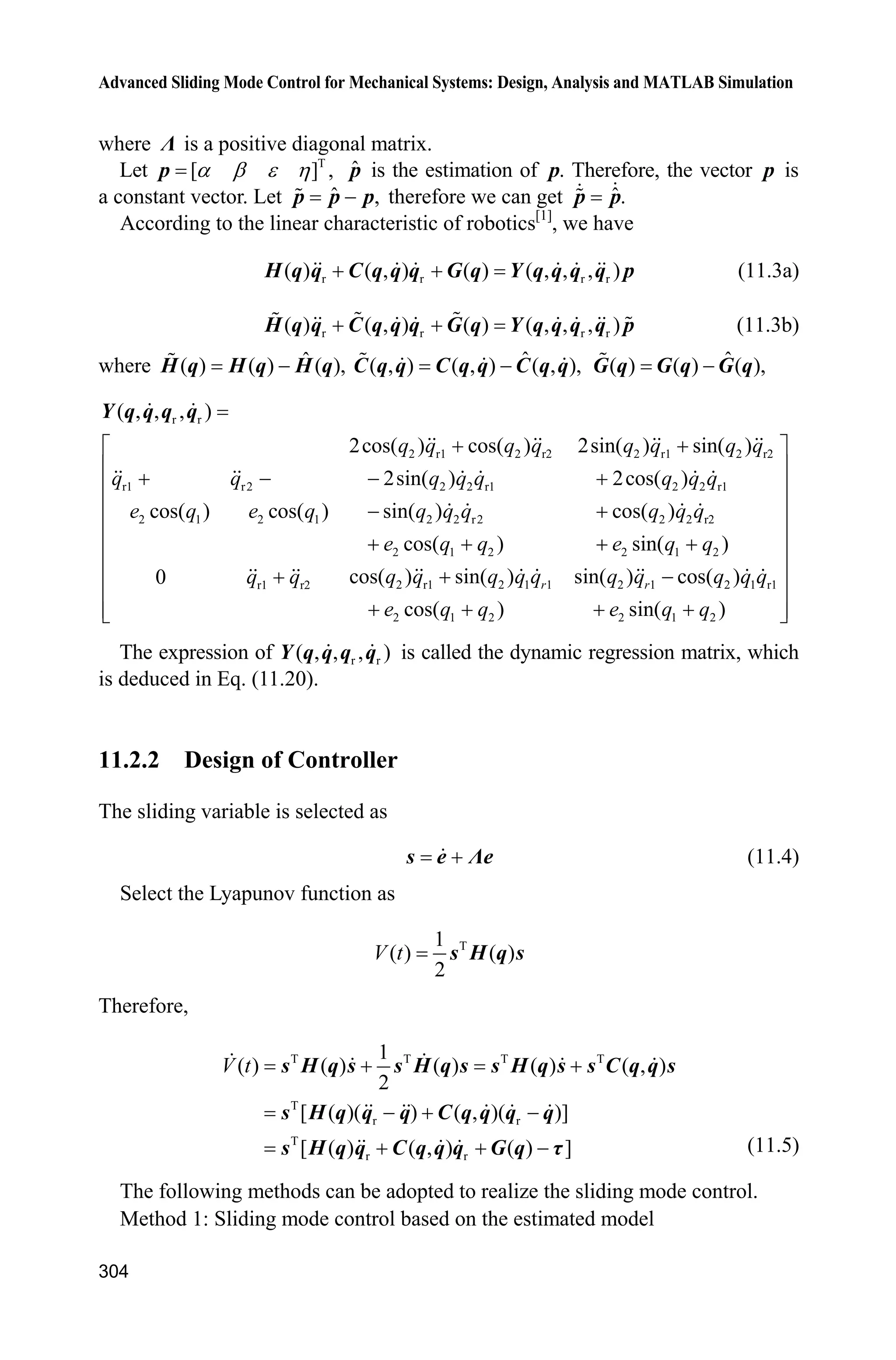
![Advanced Sliding Mode Control for Mechanical Systems: Design, Analysis and MATLAB Simulation
284
10.1.3 Simulation Example
Consider the following inverted pendulum:
1 2
2
1 2 1 1 c 1 c
2 2 2
1 c 1 c
sin cos sin /( ) cos /( )
(4/3 cos /( )) (4/3 cos /( ))
x x
g x mlx x x m m x m m
x u
l m x m m l m x m m
°
®
° ¯
where 1x and 2x are the swing angle and swing rate respectively. 2
9.8 m/sg ,
c 1kgm is the vehicle mass, m is the mass of the pendulum. l is one half of the
pendulum length, and u is the control input.
Choosing 1 ,x T the desired trajectory is d ( ) 0.1sin .t tT The initial state of
the plant is [ʌ /60,0]. We adapt control law as Eq. (10.6) and adaptive law as
Eq. (10.9), choose 15,c 0.1K and adaptive parameter 0.05.J
The structure of RBF is chosen with two input-five hidden-one output, 0.20,ijc
0.50,jb the initial value of RBF weight value is set as 0.10. The curves of
position tracking and uncertainty approximation are shown in Fig. 10.1 Fig.10.3.
Figure 10.1 Position tracking
Figure 10.2 Control input](https://image.slidesharecdn.com/advancedslidingmodecontrolformechanicalsystems-130611121131-phpapp01/75/Advanced-sliding-mode-control-for-mechanical-systems-317-2048.jpg)
![10 Neural Network Sliding Mode Control
285
Figure 10.3 ( )f x and ˆ( )f x
Simulation programs:
(1) Main Simulink program: chap10_1sim.mdl
(2) Control law program: chap10_1ctrl.m
function [sys,x0,str,ts] = spacemodel(t,x,u,flag)
switch flag,
case 0,
[sys,x0,str,ts]=mdlInitializeSizes;
case 1,
sys=mdlDerivatives(t,x,u);
case 3,
sys=mdlOutputs(t,x,u);
case {2,4,9}
sys=[];
otherwise
error(['Unhandled flag = ',num2str(flag)]);
end
function [sys,x0,str,ts]=mdlInitializeSizes
global c b n
sizes = simsizes;](https://image.slidesharecdn.com/advancedslidingmodecontrolformechanicalsystems-130611121131-phpapp01/75/Advanced-sliding-mode-control-for-mechanical-systems-318-2048.jpg)
![Advanced Sliding Mode Control for Mechanical Systems: Design, Analysis and MATLAB Simulation
286
sizes.NumContStates = 5;
sizes.NumDiscStates = 0;
sizes.NumOutputs = 2;
sizes.NumInputs = 2;
sizes.DirFeedthrough = 1;
sizes.NumSampleTimes = 0;
sys = simsizes(sizes);
x0 = 0*ones(1,5);
str = [];
ts = [];
c=0.10*ones(2,5);
b=0.50*ones(5,1);
n=15;
function sys=mdlDerivatives(t,x,u)
global c b n
e=u(1);
de=u(2);
s=n*e+de;
xi=[e;de];
h=zeros(5,1);
for j=1:1:5
h(j)=exp(-norm(xi-c(:,j))^2/(2*b(j)*b(j)));
end
gama=0.015;
W=[x(1) x(2) x(3) x(4) x(5)]';
for i=1:1:5
sys(i)=-1/gama*s*h(i);
end
function sys=mdlOutputs(t,x,u)
global c b n
e=u(1);
de=u(2);
thd=0.1*sin(t);
dthd=0.1*cos(t);
ddthd=-0.1*sin(t);
x1=thd-e;
s=n*e+de;
W=[x(1) x(2) x(3) x(4) x(5)]';
xi=[e;de];
h=zeros(5,1);
for j=1:1:5
h(j)=exp(-norm(xi-c(:,j))^2/(2*b(j)*b(j)));
end
fn=W'*h;
g=9.8;mc=1.0;m=0.1;l=0.5;
S=l*(4/3-m*(cos(x1))^2/(mc+m));
gx=cos(x1)/(mc+m);
gx=gx/S;](https://image.slidesharecdn.com/advancedslidingmodecontrolformechanicalsystems-130611121131-phpapp01/75/Advanced-sliding-mode-control-for-mechanical-systems-319-2048.jpg)
![10 Neural Network Sliding Mode Control
287
if t=1.5
xite=1.0;
else
xite=0.10;
end
ut=1/gx*(-fn+ddthd+n*de+xite*sign(s));
sys(1)=ut;
sys(2)=fn;
(3) Plant program: chap10_1plant.m
function [sys,x0,str,ts]=s_function(t,x,u,flag)
switch flag,
case 0,
[sys,x0,str,ts]=mdlInitializeSizes;
case 1,
sys=mdlDerivatives(t,x,u);
case 3,
sys=mdlOutputs(t,x,u);
case {2, 4, 9 }
sys = [];
otherwise
error(['Unhandled flag = ',num2str(flag)]);
end
function [sys,x0,str,ts]=mdlInitializeSizes
sizes = simsizes;
sizes.NumContStates = 2;
sizes.NumDiscStates = 0;
sizes.NumOutputs = 2;
sizes.NumInputs = 1;
sizes.DirFeedthrough = 0;
sizes.NumSampleTimes = 0;
sys=simsizes(sizes);
x0=[pi/60 0];
str=[];
ts=[];
function sys=mdlDerivatives(t,x,u)
g=9.8;mc=1.0;m=0.1;l=0.5;
S=l*(4/3-m*(cos(x(1)))^2/(mc+m));
fx=g*sin(x(1))-m*l*x(2)^2*cos(x(1))*sin(x(1))/(mc+m);
fx=fx/S;
gx=cos(x(1))/(mc+m);
gx=gx/S;
%%%%%%%%%
dt=0*10*sin(t);
%%%%%%%%%
sys(1)=x(2);
sys(2)=fx+gx*u+dt;
function sys=mdlOutputs(t,x,u)
g=9.8;
mc=1.0;
m=0.1;](https://image.slidesharecdn.com/advancedslidingmodecontrolformechanicalsystems-130611121131-phpapp01/75/Advanced-sliding-mode-control-for-mechanical-systems-320-2048.jpg)
![10 Neural Network Sliding Mode Control
289
we have
d q s q ȁe
d d
d d
d d d
d
( ) ( )
( )
( ) ( )
Hs H q q ȁe H q ȁe Hq
H q ȁe Cq G F IJ IJ
H q ȁe Cs C q ȁe G F IJ IJ
Cs IJ f IJ (10.12)
where d d( ) ( ) ( ) . f x H q ȁe C q ȁe G F
In engineering, ( )f x is unknown and, therefore, it is required to approximate
( )f x . The RBF network is adopted to approximate ( )f x . The network input is
selected based on the expression of ( )f x [4]
:
T T T T T
d d d[ ]x e e q q q
The controller is designed as:
v
ˆ( ) IJ f x K s (10.13)
where vK is a symmetric positive definite constant matrix, ˆ( )f x is the output of
RBF network. ˆ( )f x approximates ( )f x .
From Eqs. (10.13) and (10.12), we have
v d
v d v 0
ˆ( ) ( )
( ) ( ) ( )
Hs Cs f x K s f x IJ
K C s f x IJ K C s Ȣ (10.14)
where ˆ( ) ( ) ( )f x f x f x , 0 d( ) Ȣ f x IJ .
Select the Lyapunov function as:
T1
2
L s Hs
Therefore,
T T T T T
v 0
1 1
( 2 )
2 2
L s Hs s Hs s K s s H C s s Ȣ
T T
0 vL s Ȣ s K s
It indicates that, with v ,K the stability of control system depends on 0 ,Ȣ i.e. the
approximation precision and the magnitude of d .IJ
RBF network can be adopted to approximate ( )f x . The desired algorithm of
RBF network is:
2 2
(|| || / ),I Vi i ig x c 1,2, ,i n
*T
( )y W ij x , *T
( ) ( ) f x W ij x H](https://image.slidesharecdn.com/advancedslidingmodecontrolformechanicalsystems-130611121131-phpapp01/75/Advanced-sliding-mode-control-for-mechanical-systems-322-2048.jpg)
![Advanced Sliding Mode Control for Mechanical Systems: Design, Analysis and MATLAB Simulation
290
where x is the input state of network, T
1 2( ) [ ] ,nI I Iij x H is the appro-
ximation error of neural network, *
W is the weight vector of desired RBF network.
10.2.2 Sliding Mode Control with Respect to the Approximation
of f x( )
10.2.2.1 Design of Controller
RBF network is adopted to approximate ( ),f x therefore, the output of RBF
network is:
Tˆ ˆ( ) ( )f x W ij x (10.15)
Select
* ˆ ,W W W *
F max|| || WW
Therefore, we have
T
0 d d( ) ( ) Ȣ f x IJ W ij x İ IJ
Controller is designed as[4]
:
v
ˆ( ) IJ f x K s v (10.16)
where v is the robust element required to overcome the network approximation
error İ and the disturbance d .IJ
From Eqs. (10.16) and (10.12), we have
T
v d v 1( ) ( ) ( ) ( ) Hs K C s W ij x İ IJ v K C s Ȣ (10.17)
where T
1 d( ) ( ) . Ȣ W ij x İ IJ v
The robust element v is designed as:
N d( )sgn( )bH v s (10.18)
where N|| || Hİ , d d|| || .bIJ
10.2.2.2 Stability Analysis
Select the Lyapunov function as
T T 1
W
1 1
tr( )
2 2
L
s Hs W F W
where H and WF are positive matrices. Therefore, we have](https://image.slidesharecdn.com/advancedslidingmodecontrolformechanicalsystems-130611121131-phpapp01/75/Advanced-sliding-mode-control-for-mechanical-systems-323-2048.jpg)
![10 Neural Network Sliding Mode Control
291
T T T 1
W
1
tr( )
2
L
s Hs s Hs W F W
From Eq. (10.17), we have
T T T 1 T T
v W d
1
( 2 ) tr ( ) ( )
2
L
s K s s H C s W F W ijs s İ IJ v
We know that the manipulator has the characteristic of T
( 2 ) 0.s H C s Select
T
W ,W F ijs i.e., the adaptive rule of the network is
T
W
ˆW F ijs (10.19)
Therefore,
T T
v d( )L s K s s İ IJ v
Because
T T T T
d d d N d( ) ( ) ( ) || || ( ) 0 s İ IJ v s İ IJ s v s İ IJ s İ b
We have
0L
10.2.3 Simulation Example
The kinetic equation of the two-joint manipulator is:
d( ) ( ) ( ) ( ) H q q C q,q q G q IJ F q IJ
where
1 2 3 2 2 3 2
2 3 2 2
2 cos cos
( )
cos
p p p q p p q
p p q p
ª º
« »
¬ ¼
H q
3 2 2 3 1 2 2
3 1 2
sin ( )sin
( , )
sin 0
p q q p q q q
p q q
ª º
« »
¬ ¼
C q q
4 1 5 1 2
5 1 2
cos cos( )
( )
cos( )
p g q p g q q
p g q q
ª º
« »
¬ ¼
G q
( ) 0.02sgn( )F q q ,
T
d [0.2sin 0.2sin ]t tIJ
Let 1 2 3 4 5[ ] [2.9 0.76 0.87 3.04 0.87].p p p p pp The selection
of the Gauss function of the RBF network is very important to the control of the](https://image.slidesharecdn.com/advancedslidingmodecontrolformechanicalsystems-130611121131-phpapp01/75/Advanced-sliding-mode-control-for-mechanical-systems-324-2048.jpg)
![Advanced Sliding Mode Control for Mechanical Systems: Design, Analysis and MATLAB Simulation
292
neural network. If the parameter is not suitable, then, the available mapping of the
Gauss function cannot be obtained. Hence, the RBF network is unavailable.
Therefore, c should be selected according to the scope of network input. We
select 0.20.b The initial weight matrix of the network is selected as 0 or 0.1,
and the network input is selected as d d d[ ].z e e q q q
The initial state vector of the system is [0.09 0 0.09 0]. The desired
position commands of the two joints are 1d 0.1sinq t and 2d 0.1sinq t respectively.
The controller parameters are: v diag{20,20},K W diag{15,15},F diag{5,5}.ȁ
In the sliding robust element, select N 0.20H and d 0.10b . The controller is
given in Eq. (10.16), and the adaptive rule is given in Eq. (10.19). Simulation
results are shown in Fig.10.4Fig.10.7.
Figure 10.4 Position tracking of joints 1 and 2
Figure 10.5 Velocity tracking of joints 1 and 2](https://image.slidesharecdn.com/advancedslidingmodecontrolformechanicalsystems-130611121131-phpapp01/75/Advanced-sliding-mode-control-for-mechanical-systems-325-2048.jpg)
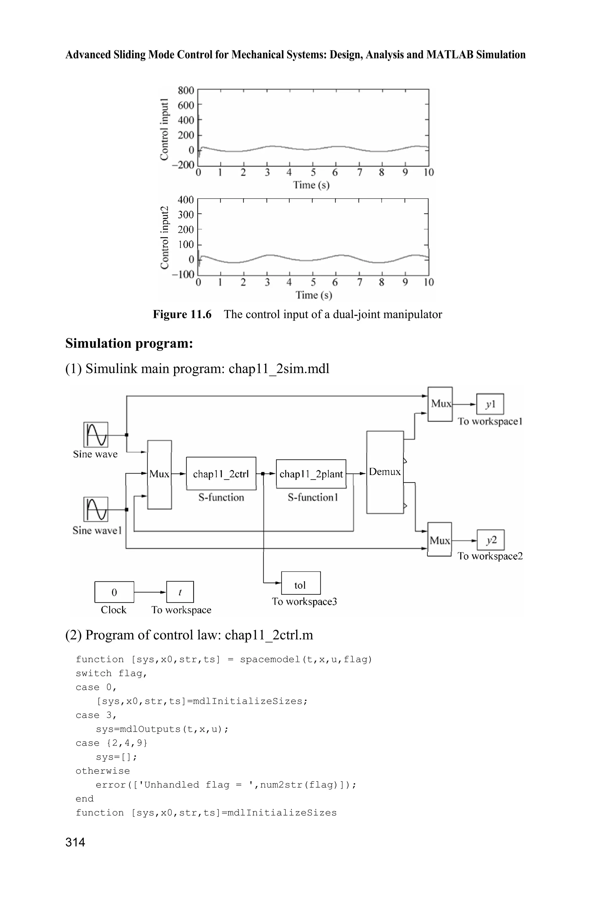
![Advanced Sliding Mode Control for Mechanical Systems: Design, Analysis and MATLAB Simulation
294
(2) Program of position commands: chap10_2input.m
function [sys,x0,str,ts] = spacemodel(t,x,u,flag)
switch flag,
case 0,
[sys,x0,str,ts]=mdlInitializeSizes;
case 1,
sys=mdlDerivatives(t,x,u);
case 3,
sys=mdlOutputs(t,x,u);
case {2,4,9}
sys=[];
otherwise
error(['Unhandled flag = ',num2str(flag)]);
end
function [sys,x0,str,ts]=mdlInitializeSizes
sizes = simsizes;
sizes.NumContStates = 0;
sizes.NumDiscStates = 0;
sizes.NumOutputs = 6;
sizes.NumInputs = 0;
sizes.DirFeedthrough = 0;
sizes.NumSampleTimes = 1;
sys = simsizes(sizes);
x0 = [];
str = [];
ts = [0 0];
function sys=mdlOutputs(t,x,u)
qd1=0.1*sin(t);
d_qd1=0.1*cos(t);
dd_qd1=-0.1*sin(t);
qd2=0.1*sin(t);
d_qd2=0.1*cos(t);
dd_qd2=-0.1*sin(t);
sys(1)=qd1;
sys(2)=d_qd1;
sys(3)=dd_qd1;
sys(4)=qd2;
sys(5)=d_qd2;
sys(6)=dd_qd2;
(3) Controller S function: chap10_2ctrl.m
function [sys,x0,str,ts] = spacemodel(t,x,u,flag)
switch flag,
case 0,
[sys,x0,str,ts]=mdlInitializeSizes;
case 1,
sys=mdlDerivatives(t,x,u);](https://image.slidesharecdn.com/advancedslidingmodecontrolformechanicalsystems-130611121131-phpapp01/75/Advanced-sliding-mode-control-for-mechanical-systems-327-2048.jpg)
![10 Neural Network Sliding Mode Control
295
case 3,
sys=mdlOutputs(t,x,u);
case {2,4,9}
sys=[];
otherwise
error(['Unhandled flag = ',num2str(flag)]);
end
function [sys,x0,str,ts]=mdlInitializeSizes
global node c b Fai
node=7;
c=0.1*[-1.5 -1 -0.5 0 0.5 1 1.5;
-1.5 -1 -0.5 0 0.5 1 1.5;
-1.5 -1 -0.5 0 0.5 1 1.5;
-1.5 -1 -0.5 0 0.5 1 1.5;
-1.5 -1 -0.5 0 0.5 1 1.5];
b=10;
Fai=5*eye(2);
sizes = simsizes;
sizes.NumContStates = 2*node;
sizes.NumDiscStates = 0;
sizes.NumOutputs = 3;
sizes.NumInputs = 11;
sizes.DirFeedthrough = 1;
sizes.NumSampleTimes = 0;
sys = simsizes(sizes);
x0 = 0.1*ones(1,2*node);
str = [];
ts = [];
function sys=mdlDerivatives(t,x,u)
global node c b Fai
qd1=u(1);
d_qd1=u(2);
dd_qd1=u(3);
qd2=u(4);
d_qd2=u(5);
dd_qd2=u(6);
q1=u(7);
d_q1=u(8);
q2=u(9);
d_q2=u(10);
q=[q1;q2];
e1=qd1-q1;
e2=qd2-q2;
de1=d_qd1-d_q1;
de2=d_qd2-d_q2;](https://image.slidesharecdn.com/advancedslidingmodecontrolformechanicalsystems-130611121131-phpapp01/75/Advanced-sliding-mode-control-for-mechanical-systems-328-2048.jpg)
![Advanced Sliding Mode Control for Mechanical Systems: Design, Analysis and MATLAB Simulation
296
e=[e1;e2];
de=[de1;de2];
S=de+Fai*e;
qd=[qd1;qd2];
dqd=[d_qd1;d_qd2];
dqr=dqd+Fai*e;
ddqd=[dd_qd1;dd_qd2];
ddqr=ddqd+Fai*de;
z1=[e(1);de(1);qd(1);dqd(1);ddqd(1)];
z2=[e(2);de(2);qd(2);dqd(2);ddqd(2)];
for j=1:1:node
h1(j)=exp(-norm(z1-c(:,j))^2/(b*b));
h2(j)=exp(-norm(z2-c(:,j))^2/(b*b));
end
Fw=15*eye(node);
for i=1:1:node
sys(i)=15*h1(i)*S(1);
sys(i+node)=15*h2(i)*S(2);
end
function sys=mdlOutputs(t,x,u)
global node c b Fai
qd1=u(1);
d_qd1=u(2);
dd_qd1=u(3);
qd2=u(4);
d_qd2=u(5);
dd_qd2=u(6);
q1=u(7);
d_q1=u(8);
q2=u(9);
d_q2=u(10);
q=[q1;q2];
e1=qd1-q1;
e2=qd2-q2;
de1=d_qd1-d_q1;
de2=d_qd2-d_q2;
e=[e1;e2];
de=[de1;de2];
S=de+Fai*e;
qd=[qd1;qd2];
dqd=[d_qd1;d_qd2];
dqr=dqd+Fai*e;](https://image.slidesharecdn.com/advancedslidingmodecontrolformechanicalsystems-130611121131-phpapp01/75/Advanced-sliding-mode-control-for-mechanical-systems-329-2048.jpg)
![10 Neural Network Sliding Mode Control
297
ddqd=[dd_qd1;dd_qd2];
ddqr=ddqd+Fai*de;
z=[e;de;qd;dqd;ddqd];
W_f1=[x(1:node)]';
W_f2=[x(node+1:node*2)]';
z1=[e(1);de(1);qd(1);dqd(1);ddqd(1)];
z2=[e(2);de(2);qd(2);dqd(2);ddqd(2)];
for j=1:1:node
h1(j)=exp(-norm(z1-c(:,j))^2/(b*b));
h2(j)=exp(-norm(z2-c(:,j))^2/(b*b));
end
fn=[W_f1*h1';
W_f2*h2'];
Kv=20*eye(2);
epN=0.20;bd=0.1;
v=-(epN+bd)*sign(S);
tol=fn+Kv*S-v;
fn_norm=norm(fn);
sys(1)=tol(1);
sys(2)=tol(2);
sys(3)=fn_norm;
(4) Program of the plant: chap10_2plant.m
function [sys,x0,str,ts]=s_function(t,x,u,flag)
switch flag,
case 0,
[sys,x0,str,ts]=mdlInitializeSizes;
case 1,
sys=mdlDerivatives(t,x,u);
case 3,
sys=mdlOutputs(t,x,u);
case {2, 4, 9 }
sys = [];
otherwise
error(['Unhandled flag = ',num2str(flag)]);
end
function [sys,x0,str,ts]=mdlInitializeSizes
global p g
sizes = simsizes;
sizes.NumContStates = 4;
sizes.NumDiscStates = 0;
sizes.NumOutputs = 5;
sizes.NumInputs =3;](https://image.slidesharecdn.com/advancedslidingmodecontrolformechanicalsystems-130611121131-phpapp01/75/Advanced-sliding-mode-control-for-mechanical-systems-330-2048.jpg)
![Advanced Sliding Mode Control for Mechanical Systems: Design, Analysis and MATLAB Simulation
298
sizes.DirFeedthrough = 0;
sizes.NumSampleTimes = 0;
sys=simsizes(sizes);
x0=[0.09 0 -0.09 0];
str=[];
ts=[];
p=[2.9 0.76 0.87 3.04 0.87];
g=9.8;
function sys=mdlDerivatives(t,x,u)
global p g
H=[p(1)+p(2)+2*p(3)*cos(x(3)) p(2)+p(3)*cos(x(3));
p(2)+p(3)*cos(x(3)) p(2)];
C=[-p(3)*x(4)*sin(x(3)) -p(3)*(x(2)+x(4))*sin(x(3));
p(3)*x(2)*sin(x(3)) 0];
G=[p(4)*g*cos(x(1))+p(5)*g*cos(x(1)+x(3));
p(5)*g*cos(x(1)+x(3))];
dq=[x(2);x(4)];
F=0.2*sign(dq);
told=[0.1*sin(t);0.1*sin(t)];
tol=u(1:2);
S=inv(H)*(tol-C*dq-G-F-told);
sys(1)=x(2);
sys(2)=S(1);
sys(3)=x(4);
sys(4)=S(2);
function sys=mdlOutputs(t,x,u)
global p g
H=[p(1)+p(2)+2*p(3)*cos(x(3)) p(2)+p(3)*cos(x(3));
p(2)+p(3)*cos(x(3)) p(2)];
C=[-p(3)*x(4)*sin(x(3)) -p(3)*(x(2)+x(4))*sin(x(3));
p(3)*x(2)*sin(x(3)) 0];
G=[p(4)*g*cos(x(1))+p(5)*g*cos(x(1)+x(3));
p(5)*g*cos(x(1)+x(3))];
dq=[x(2);x(4)];
F=0.2*sign(dq);
told=[0.1*sin(t);0.1*sin(t)];
qd1=0.1*sin(t);
d_qd1=0.1*cos(t);
dd_qd1=-0.1*sin(t);
qd2=0.1*sin(t);
d_qd2=0.1*cos(t);
dd_qd2=-0.1*sin(t);](https://image.slidesharecdn.com/advancedslidingmodecontrolformechanicalsystems-130611121131-phpapp01/75/Advanced-sliding-mode-control-for-mechanical-systems-331-2048.jpg)
![10 Neural Network Sliding Mode Control
299
q1=x(1);
d_q1=dq(1);
q2=x(3);
d_q2=dq(2);
q=[q1;q2];
e1=qd1-q1;
e2=qd2-q2;
de1=d_qd1-d_q1;
de2=d_qd2-d_q2;
e=[e1;e2];
de=[de1;de2];
Fai=5*eye(2);
dqd=[d_qd1;d_qd2];
dqr=dqd+Fai*e;
ddqd=[dd_qd1;dd_qd2];
ddqr=ddqd+Fai*de;
f=H*ddqr+C*dqr+G+F;
f_norm=norm(f);
sys(1)=x(1);
sys(2)=x(2);
sys(3)=x(3);
sys(4)=x(4);
sys(5)=f_norm;
(5) Plot program: chap10_2plot.m
close all;
figure(1);
subplot(211);
plot(t,y(:,1),'k',t,y(:,7),'r:','linewidth',2);
xlabel('time(s)');ylabel('Position tracking for link 1');
legend('Ideal position signal','Position tracking');
subplot(212);
plot(t,y(:,4),'k',t,y(:,9),'r:','linewidth',2);
xlabel('time(s)');ylabel('Position tracking for link 2');
legend('Ideal position signal','Position tracking');
figure(2);
subplot(211);
plot(t,y(:,2),'k',t,y(:,8),'r:','linewidth',2);
xlabel('time(s)');ylabel('Speed tracking for link 1');
legend('Ideal speed signal','Speed tracking');
subplot(212);
plot(t,y(:,5),'k',t,y(:,10),'r:','linewidth',2);
xlabel('time(s)');ylabel('Speed tracking for link 2');
legend('Ideal speed signal','Speed tracking');
figure(3);](https://image.slidesharecdn.com/advancedslidingmodecontrolformechanicalsystems-130611121131-phpapp01/75/Advanced-sliding-mode-control-for-mechanical-systems-332-2048.jpg)
![Advanced Sliding Mode Control for Mechanical Systems: Design, Analysis and MATLAB Simulation
300
subplot(211);
plot(t,tol1(:,1),'r','linewidth',2);
xlabel('time(s)');ylabel('control input of link 1');
subplot(212);
plot(t,tol2(:,1),'r','linewidth',2);
xlabel('time(s)');ylabel('control input of link 2');
figure(4);
plot(t,y(:,11),'k',t,y(:,12),'r:','linewidth',2);
xlabel('time(s)');ylabel('f and fn');
legend('Practical f(x)','Estimate f(x)');
References
[1] Hartman EJ, Keeler JD, Kowalski JM. Layered neural networks with Gaussian hidden
units as universal approximations. Neural computation, 1990, 2(2): 210 215
[2] Park J, Sandberg IW. Universal approximation using radial-basis-function networks. Neural
computation, 1991,3: 246 257
[3] Ge SS, Lee TH, Harris CJ. Adaptive Neural Network Control of Robotic Manipulators. World
Scientific, London, 1998
[4] Lewis FL, Liu K, Yesildirek A. Neural Net Robot Controller with Guaranteed Tracking
Performance. IEEE Transactions on Neural Networks, 1995, 6(3): 703 715](https://image.slidesharecdn.com/advancedslidingmodecontrolformechanicalsystems-130611121131-phpapp01/75/Advanced-sliding-mode-control-for-mechanical-systems-333-2048.jpg)
![11 Sliding Mode Control for Robot
Jinkun Liu
Beijing University of Aeronautics and Astronautics
P.R.China
E-mail: ljk@buaa.edu.cn
Xinhua Wang
National University of Singapore
Singapore
E-mail: wangxinhua04@gmail.com
Abstract This chapter introduces three kinds of sliding mode controllers
design for robot, including sliding mode controller design based on input-
output stability, sliding mode controller design based on computed torque
method and adaptive sliding mode controller design for manipulator.
Keywords sliding mode control, input-output stability, computed torque
method, adaptive sliding mode control, manipulator
11.1 Model of Robotic Joints
11.1.1 Model Description
In engineering, robots not only can improve productivity but also can achieve
high-strength and hazardous jobs. Manipulators are the usual plants in robotics.
Consider an n-joint manipulator as follows:
d( ) ( , ) ( ) ( ) H q q C q q q G q F q IJ IJ (11.1)
where n
q R is the angle vector, ( ) n nu
H q R is the inertia matrix, ( , ) n
C q q R
denotes the centrifugal and coriolis forces ( ) n
G q R is the gravity, ( ) n
F q R I
is the frictional force, n
IJ R is the control moment, and d
n
IJ R is the disturbance
moment.
The characteristics of the kinetic model of a manipulator[1]
:
Advanced Sliding Mode Control for Mechanical Systems
© Tsinghua University Press, Beijing and Springer-Verlag Berlin Heidelberg 201
J. Liu et al.,
2](https://image.slidesharecdn.com/advancedslidingmodecontrolformechanicalsystems-130611121131-phpapp01/75/Advanced-sliding-mode-control-for-mechanical-systems-334-2048.jpg)
![Advanced Sliding Mode Control for Mechanical Systems: Design, Analysis and MATLAB Simulation
302
(1) Kinetic model contains more number of items. The number of items included
in the equation increases with the increase in the number of robot joints.
(2) Highly nonlinearity: Each item of the equations contains non-linear factors
such as sine and cosine, et al.
(3) High degree of coupling.
(4) Model uncertainty and time-variant: The load will vary when the robot
moves the objects because the objects are not similar. Also, the Joint friction
torque will also change over time.
The characteristics of the kinetic model of a manipulator:
(1) ( )H q is a positive-definite symmetrical and bounded matrix, i.e., there
exist positive constants 1m and 2m such that 1 2( )m mI H q I ;
(2) ( , )C q q is bounded, i.e., there exists known ( )bc q such that | ( , ) |C q q
( ) || ||bc q q ;
(3) Matrix 2H C is a skew-symmetric matrix, i.e., T
( 2 ) 0,x H C x where
x is a vector;
(4) The known disturbance is satisfied with || || ,d MWIJ where MW is a known
positive constant.
A classical dual-joint rigid manipulator is shown in Fig. 11.1.
Figure 11.1 A classical dual-joint rigid manipulator
11.1.2 Model Description Example
Using the kinetic equation of a two-joint manipulator[3]
as follows:
( ) ( ) ( ) H q q C q,q q G q IJ (11.2)
where T
1 2[ ] ,q qq T
1 2[ ] ,W WIJ and
2 2 2 2
2 2
2 cos( ) 2 sin( ) cos( ) sin( )
cos( ) sin( )
q q q q
q q
D H K E H K
E H K E
ª º
« » ¬ ¼
H
2 2 2 2 2 2
2 2 1
( 2 sin( ) 2 cos( )) ( sin( ) cos( ))
( sin( ) cos( )) 0
q q q q q q
q q q
H K H K
H K
ª º
« »¬ ¼
C](https://image.slidesharecdn.com/advancedslidingmodecontrolformechanicalsystems-130611121131-phpapp01/75/Advanced-sliding-mode-control-for-mechanical-systems-335-2048.jpg)
![11 Sliding Mode Control for Robot
303
2 1 2 2 1 2 1 2 1
2 1 2 2 1 2
cos( ) sin( ) ( ) cos( )
cos( ) sin( )
e q q e q q e e q
e q q e q q
H K D E
H K
ª º
« » ¬ ¼
G
where ,D ,E H and K are constants, 2 2 2
1 1 1 1 ,c e e ce eI m l I m l m lD eIE
2
,e cem l 1 cos( ),e ce em l lH G 1 sin( ).e ce em l lK G
As an illustration, the practical parameters of a manipulator are shown in
Table 11.1.[3]
Table 11.1 Parameters of a dual-joint manipulator
1m 1l 1cl 1I em cel eI eG 1e 2e
1 kg 1 m 1/2 m 1/12 kg 3 kg 1 m 2/5 kg 0 –7/12 9.81
Let T
[ ] ,D E H Ka and ˆa is the estimation of ,a Tˆˆ ˆˆ ˆ[ ] .D E H Ka
We assume ˆ ,a a a since a is a constant vector, ˆ.a a The estimated matrices
of the above three matrices can be written respectively as:
2 2 2 2
2 2
ˆˆ ˆˆ ˆ ˆ2 cos( ) 2 sin( ) cos( ) sin( )ˆ
ˆ ˆˆ ˆcos( ) sin( )
q q q q
q q
D H K E H K
E H K E
ª º
« »
« »¬ ¼
H
2 2 2 2 2 2
2 2 1
ˆ ˆˆ ˆ( 2 sin( ) 2 cos( )) ( sin( ) cos( ))ˆ
ˆ ˆ( sin( ) cos( )) 0
q q q q q q
q q q
H K H K
H K
ª º
« »¬ ¼
C
2 1 2 2 1 2 1 2 1
2 1 2 2 1 2
ˆˆ ˆ ˆcos( ) sin( ) ( ) cos( )ˆ
ˆ ˆcos( ) sin( )
e q q e q q e e q
e q q e q q
H K D E
H K
ª º
« »
« »¬ ¼
G
11.2 Sliding Mode Control Based on Input-Output Stability
11.2.1 System Description
For the system (11.2), we assume ,D ,E H and K are the unknown constant
parameters.
Let d ( )tq denote the desired trajectory. The tracking error is
d e q q
Define
r d d( ) q q ȁ q q](https://image.slidesharecdn.com/advancedslidingmodecontrolformechanicalsystems-130611121131-phpapp01/75/Advanced-sliding-mode-control-for-mechanical-systems-336-2048.jpg)
![Advanced Sliding Mode Control for Mechanical Systems: Design, Analysis and MATLAB Simulation
304
where ȁ is a positive diagonal matrix.
Let T
[ ] ,D E H Kp ˆp is the estimation of .p Therefore, the vector p is
a constant vector. Let ˆ ,p p p therefore we can get ˆ.p p
According to the linear characteristic of robotics[1]
, we have
r r r r( ) ( , ) ( ) ( , , , ) H q q C q q q G q Y q q q q p (11.3a)
r r r r( ) ( , ) ( ) ( , , , ) H q q C q q q G q Y q q q q p (11.3b)
where ˆ( ) ( ) ( ),H q H q H q ˆ( , ) ( , ) ( , ),C q q C q q C q q ˆ( ) ( ) ( ),G q G q G q
r r
2 r1 2 r2 2 r1 2 r2
r1 r2 2 2 r1 2 2 r1
2 1 2 1 2 2 r2 2 2 r2
2 1 2 2 1 2
r1 r2
( , , , )
2cos( ) cos( ) 2sin( ) sin( )
2sin( ) 2cos( )
cos( ) cos( ) sin( ) cos( )
cos( ) sin( )
cos0
q q q q q q q q
q q q q q q q q
e q e q q q q q q q
e q q e q q
q q
Y q q q q
2 r1 2 1 1 2 1 2 1 r1
2 1 2 2 1 2
( ) sin( ) sin( ) cos( )
cos( ) sin( )
r rq q q q q q q q q q
e q q e q q
ª º
« »
« »
« »
« »
« »
« »
« »
« »¬ ¼
The expression of r r( , , , )Y q q q q is called the dynamic regression matrix, which
is deduced in Eq. (11.20).
11.2.2 Design of Controller
The sliding variable is selected as
s e ȁe (11.4)
Select the Lyapunov function as
T1
( ) ( )
2
V t s H q s
Therefore,
T T T T
T
r r
T
r r
1
( ) ( ) ( ) ( ) ( , )
2
[ ( )( ) ( , )( )]
[ ( ) ( , ) ( ) ]
V t
s H q s s H q s s H q s s C q q s
s H q q q C q q q q
s H q q C q q q G q IJ (11.5)
The following methods can be adopted to realize the sliding mode control.
Method 1: Sliding mode control based on the estimated model](https://image.slidesharecdn.com/advancedslidingmodecontrolformechanicalsystems-130611121131-phpapp01/75/Advanced-sliding-mode-control-for-mechanical-systems-337-2048.jpg)
![11 Sliding Mode Control for Robot
305
The controller is designed as
r r s
ˆ ˆˆ ( ) ( , ) ( ) IJ H q q C q q q G q IJ (11.6)
where sIJ is the robustness element to be designed
From Eqs. (11.5) and (11.6), we have:
T
r r r r s
T T
r r s r r s
ˆ ˆˆ( ) [ ( ) ( , ) ( ) ( ) ( , ) ( ) ]
[ ( ) ( , ) ( ) ] [ ( , , , ) ]
V t
s H q q C q q q G q H q q C q q q G q IJ
s H q q C q q q G q IJ s Y q q q q p IJ
where
T
1 2 3 4[ ]p p p pp , | |i ip p , 1,2,3,4i
r r( , , , ) [ ], | |ij ij ijY Y YY q q q q , 1,2i ; 1,2,3,4j
Therefore, we select
1 1 1
s
2 2 2
sgn( )
sgn( )
sgn( )
k s s
k s s
ª º
« »
¬ ¼
IJ k s s (11.7)
where
4
1
,i ij j
j
k Y p¦ 1,2.i
Therefore, we have
2 4 2 2
2
1 1 1 1
2 4 2 4 2 2
2 2
1 1 1 1 1 1
( ) sgn( )
0
i ij j i i i i
i j i i
i ij j i ij j i i
i j i j i i
V t s Y p s k s s
s Y p s Y p s s
¦¦ ¦ ¦
¦¦ ¦¦ ¦ ¦
Method 2: Sliding mode control based on the bound of model
Equation (11.5) can be written as:
T
r r
T
r r
( ) [ ( ( ) ( , ) ( ))]
[ ( , , , ) ]
V t
s IJ H q q C q q q G q
s IJ Y q q q q p
The controller can be designed as:
1 1 1
2 2 2
sgn( )
sgn( )
sgn( )
k s s
k s s
ª º
« »
« »¬ ¼
IJ k s s (11.8)
where
4
1
,i ij j
j
k Y p¦ 1,2.i](https://image.slidesharecdn.com/advancedslidingmodecontrolformechanicalsystems-130611121131-phpapp01/75/Advanced-sliding-mode-control-for-mechanical-systems-338-2048.jpg)
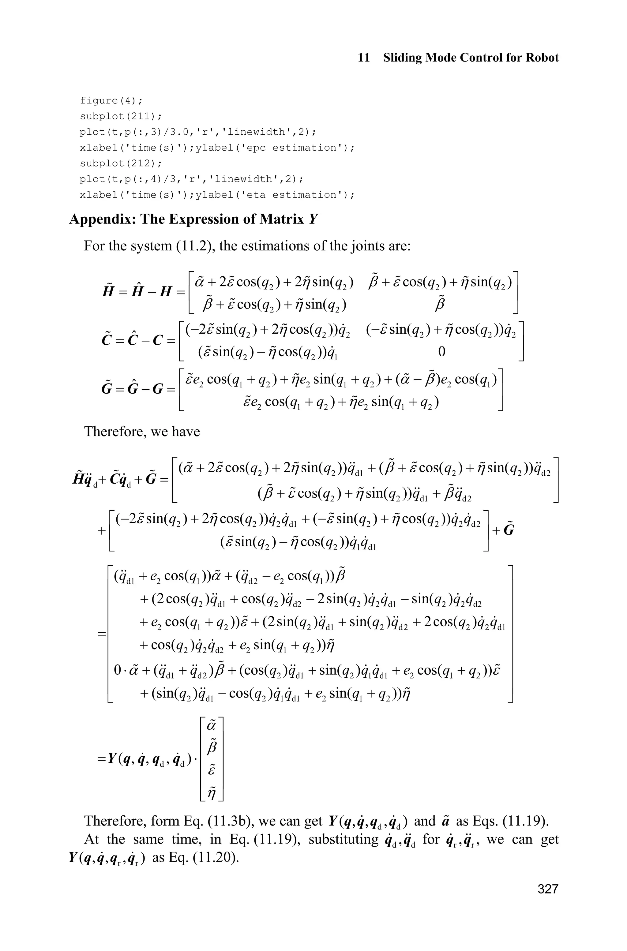
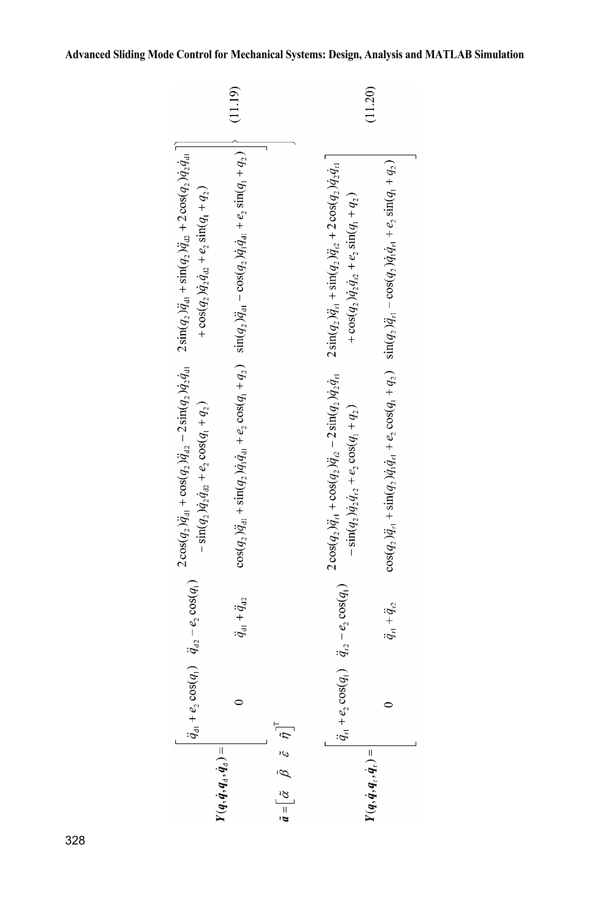
![Advanced Sliding Mode Control for Mechanical Systems: Design, Analysis and MATLAB Simulation
308
(2) Program of the controller: chap11_1ctrl.m
function [sys,x0,str,ts] = control_strategy(t,x,u,flag)
switch flag,
case 0,
[sys,x0,str,ts]=mdlInitializeSizes;
case 3,
sys=mdlOutputs(t,x,u);
case {2,4,9}
sys=[];
otherwise
error(['Unhandled flag = ',num2str(flag)]);
end
function [sys,x0,str,ts]=mdlInitializeSizes
sizes = simsizes;
sizes.NumOutputs = 2;
sizes.NumInputs = 10;
sizes.DirFeedthrough = 1;
sizes.NumSampleTimes = 0;
sys = simsizes(sizes);
x0 = [];
str = [];
ts = [];
function sys=mdlOutputs(t,x,u)
q1_d=u(1);dq1_d=u(2);ddq1_d=u(3);
q2_d=u(4);dq2_d=u(5);ddq2_d=u(6);
q1=u(7);dq1=u(8);
q2=u(9);dq2=u(10);
dq=[dq1;dq2];
p=[6.7 3.4 3.0 0]; %Practical p
ep=0.95*p; %Estimated p
alfa_p=ep(1);
beta_p=ep(2);
epc_p=ep(3);
eta_p=ep(4);
m1=1;l1=1;
lc1=1/2;I1=1/12;
g=9.8;
e1=m1*l1*lc1-I1-m1*l1^2;
e2=g/l1;
dq_d=[dq1_d,dq2_d]';
ddq_d=[ddq1_d,ddq2_d]';
e=[q1_d-q1,q2_d-q2]';
de=[dq1_d-dq1,dq2_d-dq2]';
H_p=[alfa_p+2*epc_p*cos(q2)+2*eta_p*sin(q2),beta_p+epc_p*cos(q2)+eta_p*sin(q2);
beta_p+epc_p*cos(q2)+eta_p*sin(q2),beta_p];
C_p=[(-2*epc_p*sin(q2)+2*eta_p*cos(q2))*dq2,(-epc_p*sin(q2)+eta_p*cos(q2))*dq2;
(epc_p*sin(q2)-eta_p*cos(q2))*dq1,0];](https://image.slidesharecdn.com/advancedslidingmodecontrolformechanicalsystems-130611121131-phpapp01/75/Advanced-sliding-mode-control-for-mechanical-systems-341-2048.jpg)
![11 Sliding Mode Control for Robot
309
G_p=[epc_p*e2*cos(q1+q2)+eta_p*e2*sin(q1+q2)+(alfa_p-beta_p+e1)*e2*cos(q1);
epc_p*e2*cos(q1+q2)+eta_p*e2*sin(q1+q2)];
Fai=5*eye(2);
s=de+Fai*e;
delta=0.05;
kk=1/delta;
if abs(s)delta
sats=sign(s);
else
sats=kk*s;
end
dqr=dq_d+Fai*e;
ddqr=ddq_d+Fai*de;
Y=[ddqr(1)+e2*cos(q1),ddqr(2)-e2*cos(q1),2*cos(q2)*ddqr(1)+cos(q2)*ddqr(2)
-2*sin(q2)*dq2*dqr(1)-sin(q2)*dq2*dqr(2)+e2*cos(q1+q2),2*sin(q2)*ddqr(1)+
sin(q2)*ddqr(2)+2*cos(q2)*dq2*dqr(1)+cos(q2)*dq2*dqr(2)+e2*sin(q1+q2);
0,ddqr(1)+ddqr(2),cos(q2)*ddqr(1)+sin(q2)*dq1*dqr(1)+e2*cos(q1+q2),sin(q2)
*ddqr(1)-cos(q2)*dq1*dqr(1)+e2*sin(q1+q2)];
Y_max=abs(Y)+0.10;
M=1;
if M==1
ep_up=abs(p-ep)+0.50; %Upper p-ep
k=Y_max*ep_up';
% tols=[sign(s(1)) 0;0 sign(s(2))]*k+s;
tols=[sats(1) 0;0 sats(2)]*k+s;
tol=H_p*ddqr+C_p*dqr+G_p+tols;
elseif M==2
p_up=abs(p)+0.50; %Upper p value
k_up=Y_max*p_up';
% tol=[sign(s(1)) 0;0 sign(s(2))]*k_up+s;
tol=[sats(1) 0;0 sats(2)]*k_up+s;
end
sys(1)=tol(1);
sys(2)=tol(2);
(3) Program of the plant: chap11_1plant.m
function [sys,x0,str,ts]=s_function(t,x,u,flag)
switch flag,
case 0,
[sys,x0,str,ts]=mdlInitializeSizes;
case 1,
sys=mdlDerivatives(t,x,u);
case 3,
sys=mdlOutputs(t,x,u);
case {2, 4, 9 }
sys = [];
otherwise
error(['Unhandled flag = ',num2str(flag)]);
end](https://image.slidesharecdn.com/advancedslidingmodecontrolformechanicalsystems-130611121131-phpapp01/75/Advanced-sliding-mode-control-for-mechanical-systems-342-2048.jpg)
![Advanced Sliding Mode Control for Mechanical Systems: Design, Analysis and MATLAB Simulation
310
function [sys,x0,str,ts]=mdlInitializeSizes
sizes = simsizes;
sizes.NumContStates = 4;
sizes.NumDiscStates = 0;
sizes.NumOutputs = 4;
sizes.NumInputs = 2;
sizes.DirFeedthrough = 0;
sizes.NumSampleTimes = 0;
sys=simsizes(sizes);
x0=[1.0,0,1.0,0];
str=[];
ts=[];
function sys=mdlDerivatives(t,x,u)
tol=[u(1);u(2)];
q1=x(1);
dq1=x(2);
q2=x(3);
dq2=x(4);
p=[6.7 3.4 3.0 0];
alfa=p(1);
beta=p(2);
epc=p(3);
eta=p(4);
m1=1;l1=1;
lc1=1/2;I1=1/12;
g=9.8;
e1=m1*l1*lc1-I1-m1*l1^2;
e2=g/l1;
H=[alfa+2*epc*cos(q2)+2*eta*sin(q2),beta+epc*cos(q2)+eta*sin(q2);
beta+epc*cos(q2)+eta*sin(q2),beta];
C=[(-2*epc*sin(q2)+2*eta*cos(q2))*dq2,(-epc*sin(q2)+eta*cos(q2))*dq2;
(epc*sin(q2)-eta*cos(q2))*dq1,0];
G=[epc*e2*cos(q1+q2)+eta*e2*sin(q1+q2)+(alfa-beta+e1)*e2*cos(q1);
epc*e2*cos(q1+q2)+eta*e2*sin(q1+q2)];
%robot dynamic equation as
S=inv(H)*(tol-C*[dq1;dq2]-G);
sys(1)=x(2);
sys(2)=S(1);
sys(3)=x(4);
sys(4)=S(2);
function sys=mdlOutputs(t,x,u)
sys(1)=x(1);
sys(2)=x(2);
sys(3)=x(3);
sys(4)=x(4);
(4) Program of the input command: chap11_1input.m
function [sys,x0,str,ts] = input(t,x,u,flag)
switch flag,](https://image.slidesharecdn.com/advancedslidingmodecontrolformechanicalsystems-130611121131-phpapp01/75/Advanced-sliding-mode-control-for-mechanical-systems-343-2048.jpg)
![11 Sliding Mode Control for Robot
311
case 0,
[sys,x0,str,ts]=mdlInitializeSizes;
case 3,
sys=mdlOutputs(t,x,u);
case {2,4,9}
sys=[];
otherwise
error(['Unhandled flag = ',num2str(flag)]);
end
function [sys,x0,str,ts]=mdlInitializeSizes
sizes = simsizes;
sizes.NumOutputs =6;
sizes.NumInputs = 0;
sizes.DirFeedthrough = 0;
sizes.NumSampleTimes = 0;
sys = simsizes(sizes);
x0 = [];
str = [];
ts = [];
function sys=mdlOutputs(t,x,u)
q1_d=sin(2*pi*t);
q2_d=sin(2*pi*t);
dq1_d=2*pi*cos(2*pi*t);
dq2_d=2*pi*cos(2*pi*t);
ddq1_d=-(2*pi)^2*sin(2*pi*t);
ddq2_d=-(2*pi)^2*sin(2*pi*t);
sys(1)=q1_d;
sys(2)=dq1_d;
sys(3)=ddq1_d;
sys(4)=q2_d;
sys(5)=dq2_d;
sys(6)=ddq2_d;
(5) Plot program: chap11_1plot.m
close all;
figure(1);
subplot(211);
plot(t,qd(:,1),'k',t,q(:,1),'r:','linewidth',2);
xlabel('time(s)');ylabel('Position tracking of link 1');
legend('Ideal position signal','Tracking position signal');
subplot(212);
plot(t,qd(:,2),'k',t,q(:,2),'r:','linewidth',2);
xlabel('time(s)');ylabel('Speed tracking of link 1');
legend('Ideal speed signal','Tracking speed signal');
figure(2);
subplot(211);
plot(t,qd(:,4),'k',t,q(:,3),'r:','linewidth',2);
xlabel('time(s)');ylabel('Position tracking of link 2');
legend('Ideal position signal','Tracking position signal');
subplot(212);](https://image.slidesharecdn.com/advancedslidingmodecontrolformechanicalsystems-130611121131-phpapp01/75/Advanced-sliding-mode-control-for-mechanical-systems-344-2048.jpg)
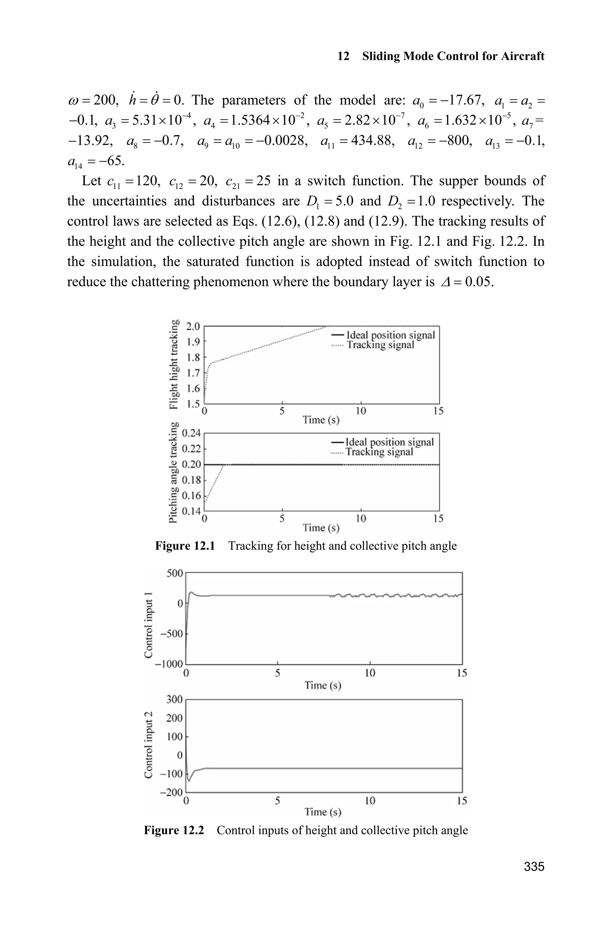
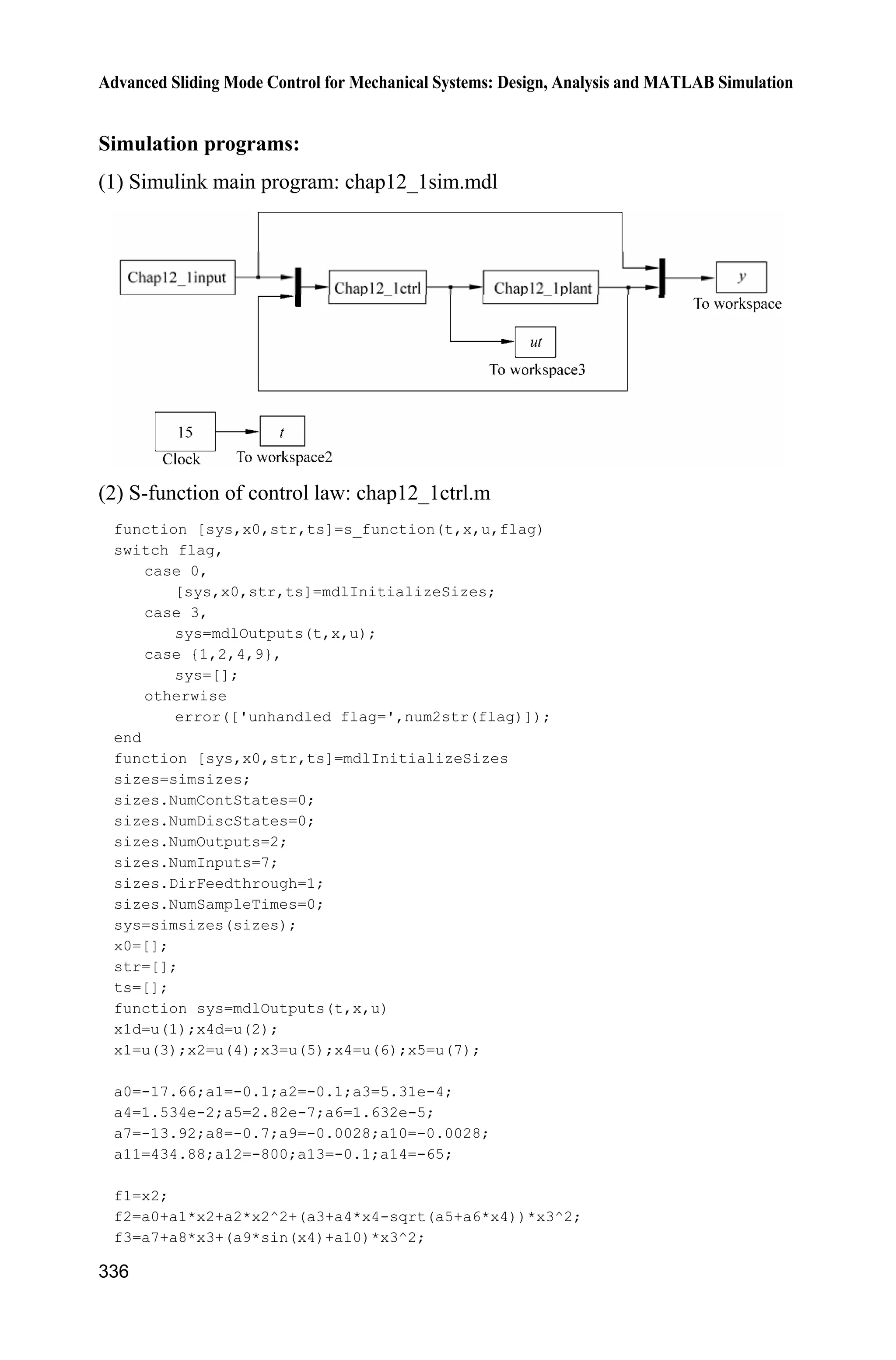
![ˆ ˆˆ , IJ H q v C q q q G q (11.9)
where v is the auxiliary control input, ˆ ( )H q , ˆ( , )C q q and ˆ( )G q are the respective
estimations of ,H C and G by using inertial parameter ˆp of manipulator.
Substituting Eq. (11.9) into Eq. (11.1), neglecting ( )F q and d ,W considering
Eq. (11.3b), we have
ˆ ˆˆ( ) ( , ) ( ) ( ) ( , ) ( ) H q q C q q q G q H q v C q q q G q (11.10)
i.e.
ˆ ˆ ˆ( ) [ ( ) ( , ) ( )] ( ) ( , , ) Hq H q v H q q C q q q G q H q v Y q q q p
where ˆ ,H H H ˆ,C C C ˆ,G G G ˆ.p p p
If the parameter estimation ˆp makes ˆ ( )H q invertible, then the above equation
can be written as:
1ˆ( ( )) ( , , )
q v H q Y q q q p v d
where 1ˆˆ( , , , ) ( ( )) ( , , ),
ij q q q p H q Y q q q ˆ( , , , ) .ij q q q p p d
The sliding variable can be selected as:
s e ȁe (11.11)
where d ,e q q d ,e q q T
1 2[ ] , ns s ss ȁ is a positive diagonal matrix.](https://image.slidesharecdn.com/advancedslidingmodecontrolformechanicalsystems-130611121131-phpapp01/75/Advanced-sliding-mode-control-for-mechanical-systems-348-2048.jpg)
![11 Sliding Mode Control for Robot
313
Therefore,
d d( ) s e ȁe q q ȁe q v d ȁe
Select
d v q ȁe d (11.12)
where ( )sgn( ), || || ,d d Ș s d d 0.!Ș
Therefore, we have
s d d
The Lyapunov function is selected as T1
,
2
V s s therefore, we have
T T T T T
( ) sgn( ) sgn( ) || || 0V s s s d d s d ds s Șs s Ș s
From the controller, the more precise the estimation of ˆp is, the smaller
are || ||p and ,d and smaller is the chattering of the sliding mode.
11.3.2 Simulation Example
We consider the plant as Eq. (11.2) The initial state vector is T
[0 0 0 0] . The
sliding mode controller is given in Eqs. (11.9) and (11.12). The desired trajectory
is d1 sin ,q t d2 sin .q t ˆ 0.6 ,H H ˆ 0.6 ,C C ˆ 0.6 ,G G 30,d 0.10,K
25 0
.
0 25
ª º
« »
¬ ¼
ȁ The simulation results are shown in Fig. 11.5 and Fig. 11.6.
Figure 11.5 The position tracking of a dual-joint manipulator](https://image.slidesharecdn.com/advancedslidingmodecontrolformechanicalsystems-130611121131-phpapp01/75/Advanced-sliding-mode-control-for-mechanical-systems-349-2048.jpg)
![Advanced Sliding Mode Control for Mechanical Systems: Design, Analysis and MATLAB Simulation
314
Figure 11.6 The control input of a dual-joint manipulator
Simulation program:
(1) Simulink main program: chap11_2sim.mdl
(2) Program of control law: chap11_2ctrl.m
function [sys,x0,str,ts] = spacemodel(t,x,u,flag)
switch flag,
case 0,
[sys,x0,str,ts]=mdlInitializeSizes;
case 3,
sys=mdlOutputs(t,x,u);
case {2,4,9}
sys=[];
otherwise
error(['Unhandled flag = ',num2str(flag)]);
end
function [sys,x0,str,ts]=mdlInitializeSizes](https://image.slidesharecdn.com/advancedslidingmodecontrolformechanicalsystems-130611121131-phpapp01/75/Advanced-sliding-mode-control-for-mechanical-systems-350-2048.jpg)
![11 Sliding Mode Control for Robot
315
global nmn
nmn=25*eye(2);
sizes = simsizes;
sizes.NumContStates = 0;
sizes.NumDiscStates = 0;
sizes.NumOutputs = 2;
sizes.NumInputs = 6;
sizes.DirFeedthrough = 1;
sizes.NumSampleTimes = 1;
sys = simsizes(sizes);
x0 = [];
str = [];
ts = [0 0];
function sys=mdlOutputs(t,x,u)
global nmn
qd1=u(1);
dqd1=cos(t);
ddqd1=-sin(t);
qd2=u(2);
dqd2=cos(t);
ddqd2=-sin(t);
ddqd=[ddqd1;ddqd2];
dqd=[dqd1;dqd2];
ddqd=[ddqd1;ddqd2];
q1=u(3);dq1=u(4);
q2=u(5);dq2=u(6);
dq=[dq1;dq2];
e1=qd1-q1;
e2=qd2-q2;
e=[e1;e2];
de1=dqd1-dq1;
de2=dqd2-dq2;
de=[de1;de2];
alfa=6.7;beta=3.4;
epc=3.0;eta=0;
m1=1;l1=1;
lc1=1/2;I1=1/12;
g=9.8;
e1=m1*l1*lc1-I1-m1*l1^2;
e2=g/l1;
H=[alfa+2*epc*cos(q2)+2*eta*sin(q2),beta+epc*cos(q2)+eta*sin(q2);
beta+epc*cos(q2)+eta*sin(q2),beta];
C=[(-2*epc*sin(q2)+2*eta*cos(q2))*dq2,(-epc*sin(q2)+eta*cos(q2))*dq2;
(epc*sin(q2)-eta*cos(q2))*dq1,0];
G=[epc*e2*cos(q1+q2)+eta*e2*sin(q1+q2)+(alfa-beta+e1)*e2*cos(q1);
epc*e2*cos(q1+q2)+eta*e2*sin(q1+q2)];
H0=0.6*H;
C0=0.6*C;
G0=0.6*G;](https://image.slidesharecdn.com/advancedslidingmodecontrolformechanicalsystems-130611121131-phpapp01/75/Advanced-sliding-mode-control-for-mechanical-systems-351-2048.jpg)
![Advanced Sliding Mode Control for Mechanical Systems: Design, Analysis and MATLAB Simulation
316
s=de+nmn*e;
d_up=30;
xite=0.10;
M=2;
if M==1
d=(d_up+xite)*sign(s);
elseif M==2 %Saturated function
delta=0.05;
kk=1/delta;
if abs(s)delta
sats=sign(s);
else
sats=kk*s;
end
end
d=(d_up+xite)*sats;
v=ddqd+nmn*de+d;
tol=H0*v+C0*dq+G0;
sys(1)=tol(1);
sys(2)=tol(2);
(3) Program of the plant: chap11_2plant.m
function [sys,x0,str,ts]=s_function(t,x,u,flag)
switch flag,
case 0,
[sys,x0,str,ts]=mdlInitializeSizes;
case 1,
sys=mdlDerivatives(t,x,u);
case 3,
sys=mdlOutputs(t,x,u);
case {2, 4, 9 }
sys = [];
otherwise
error(['Unhandled flag = ',num2str(flag)]);
end
function [sys,x0,str,ts]=mdlInitializeSizes
sizes = simsizes;
sizes.NumContStates = 4;
sizes.NumDiscStates = 0;
sizes.NumOutputs = 4;
sizes.NumInputs = 2;
sizes.DirFeedthrough = 0;
sizes.NumSampleTimes = 0;
sys=simsizes(sizes);
x0=[0;0;0;0];
str=[];
ts=[];
function sys=mdlDerivatives(t,x,u)
q1=x(1);dq1=x(2);](https://image.slidesharecdn.com/advancedslidingmodecontrolformechanicalsystems-130611121131-phpapp01/75/Advanced-sliding-mode-control-for-mechanical-systems-352-2048.jpg)
![11 Sliding Mode Control for Robot
317
q2=x(3);dq2=x(4);
dq=[dq1;dq2];
% The model is given by Slotine and Weiping Li(MIT 1987)
alfa=6.7;beta=3.4;
epc=3.0;eta=0;
m1=1;l1=1;
lc1=1/2;I1=1/12;
g=9.8;
e1=m1*l1*lc1-I1-m1*l1^2;
e2=g/l1;
H=[alfa+2*epc*cos(q2)+2*eta*sin(q2),beta+epc*cos(q2)+eta*sin(q2);
beta+epc*cos(q2)+eta*sin(q2),beta];
C=[(-2*epc*sin(q2)+2*eta*cos(q2))*dq2,(-epc*sin(q2)+eta*cos(q2))*dq2;
(epc*sin(q2)-eta*cos(q2))*dq1,0];
G=[epc*e2*cos(q1+q2)+eta*e2*sin(q1+q2)+(alfa-beta+e1)*e2*cos(q1);
epc*e2*cos(q1+q2)+eta*e2*sin(q1+q2)];
tol(1)=u(1);
tol(2)=u(2);
ddq=inv(H)*(tol'-C*dq-G);
sys(1)=x(2);
sys(2)=ddq(1);
sys(3)=x(4);
sys(4)=ddq(2);
function sys=mdlOutputs(t,x,u)
sys(1)=x(1);
sys(2)=x(2);
sys(3)=x(3);
sys(4)=x(4);
(4) Plot program: chap11_2plot.m
close all;
figure(1);
subplot(211);
plot(t,y1(:,1),'k',t,y1(:,2),'r:','linewidth',2);
xlabel('time(s)');ylabel('Position tracking of joint 1');
legend('Ideal position signal','tracking signal');
subplot(212);
plot(t,y2(:,1),'k',t,y2(:,2),'r:','linewidth',2);
xlabel('time(s)');ylabel('Position tracking of joint 2');
legend('Ideal position signal','tracking signal');
figure(2);
subplot(211);
plot(t,tol(:,1),'r','linewidth',2);
xlabel('time(s)');ylabel('Control input 1');
subplot(212);
plot(t,tol(:,2),'r','linewidth',2);
xlabel('time(s)');ylabel('Control input 2');](https://image.slidesharecdn.com/advancedslidingmodecontrolformechanicalsystems-130611121131-phpapp01/75/Advanced-sliding-mode-control-for-mechanical-systems-353-2048.jpg)
![Advanced Sliding Mode Control for Mechanical Systems: Design, Analysis and MATLAB Simulation
318
11.4 Adaptive Sliding Mode Control for Manipulator
We discussed an adaptive sliding mode controller design method for the manipulator.
Refer to paper[2]
.
11.4.1 Adaptive Sliding Mode Controller
For the system (11.2), we assume ,D ,E H and K are the unknown constant
parameters.
Let d( ) ( ) ( )t t tq q q be the tracking error, and denote
r d ,q q ȁq r d q q ȁq (11.13)
where 1
2
0
,
0
O
O
ª º
« »
¬ ¼
ȁ 0,iO ! 1,2.i
Define the sliding variable as:
= +s q ȁq (11.14)
Slotine et al. proposed the controller[2,3]
as:
r r D
ˆ ˆˆ ( ) ( , ) ( ) IJ H q q C q q q G q K s (11.15)
where d1
D
d2
0
,
0
ª º
« »
¬ ¼
k
k
K d 0,ik ! 1,2.i
Because H is a positive-definite matrix, we select the Lyapunov function as
T T1 1
( )
2 2
V t s Hs a īa (11.16)
where
1
2
3
4
0 0 0
0 0 0
,
0 0 0
0 0 0
J
J
J
J
ª º
« »
« »
« »
« »
¬ ¼
ī 0,iJ ! 1,2,3,4.i
Therefore, we have
T T T T T T
T T T
r
T T T
r r
1 1
( ) ( )
2 2
1
( )
2
1
( ( ) )
2
V t
rs Hs s Hs a īa s Hq Hq s Hs a īa
s IJ Cq G Hq s Hs a īa
s IJ C s q G Hq s Hs a īa
From Eq. (11.15), we can get](https://image.slidesharecdn.com/advancedslidingmodecontrolformechanicalsystems-130611121131-phpapp01/75/Advanced-sliding-mode-control-for-mechanical-systems-354-2048.jpg)
![11 Sliding Mode Control for Robot
319
T T T
r r D r r
T T T
r r D
1ˆ ˆˆ( ) ( ( ) )
2
1
( )
2
V t
s Hq Cq G K s C s q G - Hq s Hs a īa
s Hq Cq G K s Cs s Hs a īa
From the linear characteristic of the kinetic equation of the manipulator[3]
, just
like Eq. (11.3b), it follows:
r r r r( , , , ) Hq Cq G Y q q q q a (11.17)
Therefore,
T T T
D
T T T
D
T T T T T T
D D
T T T
D
1
( ) ( )
2
1
( ) ( 2 )
2
( )
( )
V t
s Ya K s Cs s Hs a īa
s Ya K s s H C s a īa
s Ya K s a īa a Y s s K s a īa
a Y s īa s K s
Adaptive rule[2, 3]
was designed by slotine et al. as follows:
1 T
ˆ
a ī Y s (11.18)
Therefore,
T
D( ) 0V t s K s
Then 0oq as .t o f
11.4.2 Simulation Example
We consider the plant as Eq. (11.2). The desired trajectories of the two arms are
d1 sin(2ʌ )q t and d2 sin(2ʌ )q t respectively. The controller and the adaptive rule
are shown in Eqs. (11.15) and (11.18) respectively. r r( , , , )Y q q q q is given in
Eq. (11.20). Select
5 0
,
0 5
ª º
« »
¬ ¼
ȁ D
100 0
,
0 100
ª º
« »
¬ ¼
K
1 0 0 0
0 1 0 0
0 0 1 0
0 0 0 1
ª º
« »
« »
« »
« »
¬ ¼
ī (See the
appendix). The simulation results are shown in Fig. 11.7 Fig. 11.10. We can see
from Fig. 11.9 and Fig. 11.10 that the effects of identification to ,D ,E ,H and
K are not satisfied. The convergence of trajectories tracking can be guaranteed by
the adaptive rule. However, the estimations cannot converge to the desired values,
the reason is explained in Section 6.1. The information of desired trajectories must
be abundant[2]
to improve the estimation precision.](https://image.slidesharecdn.com/advancedslidingmodecontrolformechanicalsystems-130611121131-phpapp01/75/Advanced-sliding-mode-control-for-mechanical-systems-355-2048.jpg)
![11 Sliding Mode Control for Robot
321
Figure 11.10 The estimations of H and K
Simulation programs:
(1) Simulink main program: chap11_3sim.mdl
(2) Program of input command: chap11_3input.m
function [sys,x0,str,ts] = input(t,x,u,flag)
switch flag,
case 0,
[sys,x0,str,ts]=mdlInitializeSizes;
case 3,
sys=mdlOutputs(t,x,u);
case {2,4,9}
sys=[];
otherwise
error(['Unhandled flag = ',num2str(flag)]);
end](https://image.slidesharecdn.com/advancedslidingmodecontrolformechanicalsystems-130611121131-phpapp01/75/Advanced-sliding-mode-control-for-mechanical-systems-357-2048.jpg)
![Advanced Sliding Mode Control for Mechanical Systems: Design, Analysis and MATLAB Simulation
322
function [sys,x0,str,ts]=mdlInitializeSizes
sizes = simsizes;
sizes.NumOutputs =6;
sizes.NumInputs = 0;
sizes.DirFeedthrough = 0;
sizes.NumSampleTimes = 0;
sys = simsizes(sizes);
x0 = [];
str = [];
ts = [];
function sys=mdlOutputs(t,x,u)
q1_d=sin(2*pi*t);
q2_d=sin(2*pi*t);
dq1_d=2*pi*cos(2*pi*t);
dq2_d=2*pi*cos(2*pi*t);
ddq1_d=-(2*pi)^2*sin(2*pi*t);
ddq2_d=-(2*pi)^2*sin(2*pi*t);
sys(1)=q1_d;
sys(2)=dq1_d;
sys(3)=ddq1_d;
sys(4)=q2_d;
sys(5)=dq2_d;
sys(6)=ddq2_d;
(3) Program of controller: chap11_3ctrl.m
function [sys,x0,str,ts] = control_strategy(t,x,u,flag)
switch flag,
case 0,
[sys,x0,str,ts]=mdlInitializeSizes;
case 3,
sys=mdlOutputs(t,x,u);
case {2,4,9}
sys=[];
otherwise
error(['Unhandled flag = ',num2str(flag)]);
end
function [sys,x0,str,ts]=mdlInitializeSizes
sizes = simsizes;
sizes.NumOutputs = 2;
sizes.NumInputs = 14;
sizes.DirFeedthrough = 1;
sizes.NumSampleTimes = 0;
sys = simsizes(sizes);
x0 = [];
str = [];
ts = [];
function sys=mdlOutputs(t,x,u)
q1_d=u(1);dq1_d=u(2);ddq1_d=u(3);](https://image.slidesharecdn.com/advancedslidingmodecontrolformechanicalsystems-130611121131-phpapp01/75/Advanced-sliding-mode-control-for-mechanical-systems-358-2048.jpg)
![11 Sliding Mode Control for Robot
323
q2_d=u(4);dq2_d=u(5);ddq2_d=u(6);
q1=u(7);dq1=u(8);
q2=u(9);dq2=u(10);
alfa_p=u(11);
beta_p=u(12);
epc_p=u(13);
eta_p=u(14);
m1=1;l1=1;
lc1=1/2;I1=1/12;
g=9.8;
e1=m1*l1*lc1-I1-m1*l1^2;
e2=g/l1;
dq_d=[dq1_d,dq2_d]';
ddq_d=[ddq1_d,ddq2_d]';
q_error=[q1-q1_d,q2-q2_d]';
dq_error=[dq1-dq1_d,dq2-dq2_d]';
H_p=[alfa_p+2*epc_p*cos(q2)+2*eta_p*sin(q2),beta_p+epc_p*cos(q2)+eta_p*sin(q2);
beta_p+epc_p*cos(q2)+eta_p*sin(q2),beta_p];
C_p=[(-2*epc_p*sin(q2)+2*eta_p*cos(q2))*dq2,(-epc_p*sin(q2)+eta_p*cos(q2))*dq2;
(epc_p*sin(q2)-eta_p*cos(q2))*dq1,0];
G_p=[epc_p*e2*cos(q1+q2)+eta_p*e2*sin(q1+q2)+(alfa_p-beta_p+e1)*e2*cos(q1);
epc_p*e2*cos(q1+q2)+eta_p*e2*sin(q1+q2)];
Fai=5*eye(2);
dqr=dq_d-Fai*q_error;
ddqr=ddq_d-Fai*dq_error;
s=Fai*q_error+dq_error;
Kd=100*eye(2);
tol=H_p*ddqr+C_p*dqr+G_p-Kd*s;
sys(1)=tol(1);
sys(2)=tol(2);
(4) Program of adaptive rule: chap11_3adapt.m
function [sys,x0,str,ts]=para_estimate(t,x,u,flag)
switch flag,
case 0,
[sys,x0,str,ts]=mdlInitializeSizes;
case 1,
sys=mdlDerivatives(t,x,u);
case 3,
sys=mdlOutputs(t,x,u);
case {2, 4, 9 }
sys = [];](https://image.slidesharecdn.com/advancedslidingmodecontrolformechanicalsystems-130611121131-phpapp01/75/Advanced-sliding-mode-control-for-mechanical-systems-359-2048.jpg)
![Advanced Sliding Mode Control for Mechanical Systems: Design, Analysis and MATLAB Simulation
324
otherwise
error(['Unhandled flag = ',num2str(flag)]);
end
function [sys,x0,str,ts]=mdlInitializeSizes
sizes = simsizes;
sizes.NumContStates = 4;
sizes.NumDiscStates = 0;
sizes.NumOutputs = 4;
sizes.NumInputs = 10;
sizes.DirFeedthrough = 1;
sizes.NumSampleTimes = 0;
sys=simsizes(sizes);
x0=[4.1,1.9,1.7,0];
str=[];
ts=[];
function sys=mdlDerivatives(t,x,u)
g=9.8;l1=1;
e2=g/l1;
gama=eye(4);
q1_d=u(1);dq1_d=u(2);ddq1_d=u(3);
q2_d=u(4);dq2_d=u(5);ddq2_d=u(6);
q1=u(7);dq1=u(8);
q2=u(9);dq2=u(10);
q_error=[q1-q1_d,q2-q2_d]';
dq_error=[dq1-dq1_d,dq2-dq2_d]';
Fai=5*eye(2);
s=Fai*q_error+dq_error;
ddq_d=[ddq1_d,ddq2_d]';
dq_d=[dq1_d,dq2_d]';
dqr=dq_d-Fai*q_error;
ddqr=ddq_d-Fai*dq_error;
Y=[ddqr(1)+e2*cos(q1),ddqr(2)-e2*cos(q1),2*cos(q2)*ddqr(1)+cos(q2)*ddqr(2)
-2*sin(q2)*dq2*dqr(1)-sin(q2)*dq2*dqr(2)+e2*cos(q1+q2),2*sin(q2)*ddqr(1)
+sin(q2)*ddqr(2)+2*cos(q2)*dq2*dqr(1)+cos(q2)*dq2*dqr(2)+e2*sin(q1+q2);
0,ddqr(1)+ddqr(2),cos(q2)*ddqr(1)+sin(q2)*dq1*dqr(1)+e2*cos(q1+q2),
sin(q2)*ddqr(1)-cos(q2)*dq1*dqr(1)+e2*sin(q1+q2)];
A_law=-inv(gama)*Y'*s; %Adaptive law
% The parameter update law is proposed by Slotine and Weiping Li(MIT 1987)
for i=1:1:4
sys(i)=A_law(i);
end
function sys=mdlOutputs(t,x,u)](https://image.slidesharecdn.com/advancedslidingmodecontrolformechanicalsystems-130611121131-phpapp01/75/Advanced-sliding-mode-control-for-mechanical-systems-360-2048.jpg)
![11 Sliding Mode Control for Robot
325
sys(1)=x(1);
sys(2)=x(2);
sys(3)=x(3);
sys(4)=x(4);
(5) Program of the plant: chap11_3plant.m
function [sys,x0,str,ts]=s_function(t,x,u,flag)
switch flag,
case 0,
[sys,x0,str,ts]=mdlInitializeSizes;
case 1,
sys=mdlDerivatives(t,x,u);
case 3,
sys=mdlOutputs(t,x,u);
case {2, 4, 9 }
sys = [];
otherwise
error(['Unhandled flag = ',num2str(flag)]);
end
function [sys,x0,str,ts]=mdlInitializeSizes
sizes = simsizes;
sizes.NumContStates = 4;
sizes.NumDiscStates = 0;
sizes.NumOutputs = 4;
sizes.NumInputs = 2;
sizes.DirFeedthrough = 0;
sizes.NumSampleTimes = 0;
sys=simsizes(sizes);
x0=[1.0,0,1.0,0];
str=[];
ts=[];
function sys=mdlDerivatives(t,x,u)
tol=[u(1);u(2)];
q1=x(1);
dq1=x(2);
q2=x(3);
dq2=x(4);
alfa=6.7;
beta=3.4;
epc=3.0;
eta=0;
m1=1;l1=1;
lc1=1/2;I1=1/12;
g=9.8;
e1=m1*l1*lc1-I1-m1*l1^2;
e2=g/l1;](https://image.slidesharecdn.com/advancedslidingmodecontrolformechanicalsystems-130611121131-phpapp01/75/Advanced-sliding-mode-control-for-mechanical-systems-361-2048.jpg)
![Advanced Sliding Mode Control for Mechanical Systems: Design, Analysis and MATLAB Simulation
326
H=[alfa+2*epc*cos(q2)+2*eta*sin(q2),beta+epc*cos(q2)+eta*sin(q2);
beta+epc*cos(q2)+eta*sin(q2),beta];
C=[(-2*epc*sin(q2)+2*eta*cos(q2))*dq2,(-epc*sin(q2)+eta*cos(q2))*dq2;
(epc*sin(q2)-eta*cos(q2))*dq1,0];
G=[epc*e2*cos(q1+q2)+eta*e2*sin(q1+q2)+(alfa-beta+e1)*e2*cos(q1);
epc*e2*cos(q1+q2)+eta*e2*sin(q1+q2)];
S=inv(H)*(tol-C*[dq1;dq2]-G);
sys(1)=x(2);
sys(2)=S(1);
sys(3)=x(4);
sys(4)=S(2);
function sys=mdlOutputs(t,x,u)
sys(1)=x(1);
sys(2)=x(2);
sys(3)=x(3);
sys(4)=x(4);
(6) Plot program: chap11_3plot.m
close all;
figure(1);
subplot(211);
plot(t,qd(:,1),'k',t,q(:,1),'r:','linewidth',2);
xlabel('time(s)');ylabel('position tracking of link 1');
legend('ideal signal','tracking signal');
subplot(212);
plot(t,qd(:,2),'k',t,q(:,2),'r:','linewidth',2);
xlabel('time(s)');ylabel('speed tracking of link 1');
legend('ideal signal','tracking signal');
figure(2);
subplot(211);
plot(t,qd(:,4),'k',t,q(:,3),'r:','linewidth',2);
xlabel('time(s)');ylabel('position tracking of link 2');
legend('ideal signal','tracking signal');
subplot(212);
plot(t,qd(:,5),'k',t,q(:,4),'r:','linewidth',2);
xlabel('time(s)');ylabel('speed tracking of link 2');
legend('ideal signal','tracking signal');
figure(3);
subplot(211);
plot(t,p(:,1)/6.7,'r','linewidth',2);
xlabel('time(s)');ylabel('alfa estimation');
subplot(212);
plot(t,p(:,2)/3.4,'r','linewidth',2);
xlabel('time(s)');ylabel('beta estimation');](https://image.slidesharecdn.com/advancedslidingmodecontrolformechanicalsystems-130611121131-phpapp01/75/Advanced-sliding-mode-control-for-mechanical-systems-362-2048.jpg)
![11 Sliding Mode Control for Robot
329
References
[1] Sadao kawamura, Mikhail Svinin. eds., Advances in Robot Control: From Everyday physics
to Human-like Movements. Springer, 2006
[2] Slotine JE, Li WP. On the adaptive control of robot manipulators. The Interational Journal
of Robotics Research, 1987, 6(3): 49 59
[3] Slotine JE, Li WP. Applied Non Linear Control. Prentice Hall, 1991](https://image.slidesharecdn.com/advancedslidingmodecontrolformechanicalsystems-130611121131-phpapp01/75/Advanced-sliding-mode-control-for-mechanical-systems-365-2048.jpg)
![12 Sliding Mode Control for Aircraft
Jinkun Liu
Beijing University of Aeronautics and Astronautics
P.R.China
E-mail: ljk@buaa.edu.cn
Xinhua Wang
National University of Singapore
Singapore
E-mail: wangxinhua04@gmail.com
Abstract This chapter introduces two kinds of sliding mode controllers for
aircrafts. They are a sliding mode controller for helicopter and a sliding mode
controller for an uncertain VTOL aircraft. Stability analysis and simulation
examples are given.
Keywords sliding mode control, helicopter, VTOL aircraft
12.1 Sliding Mode Control for a Helicopter
12.1.1 Mathematical Model of a Helicopter
The control system of a helicopter is a multiple input multiple output (MIMO)
system. The nonlinear motion characteristics of helicopter are obvious. Moreover,
the stability, operation, and maneuverability are relatively worse. The height of a
helicopter varies according to the pitch angle. Ignoring the ground effect, the
kinetic equation of a helicopter is described as follows:
1 1 2 2
T T
1 2 1 4
( ) ( ) ( )
[ ] [ ]
½
¾
¿
u u
y y x x
x f x g x g x
y
(12.1)
where T
1( ) [0 0 1 0 0] ,g x T
2 ( ) [0 0 0 0 1] ,g x T
1 2 3 4 5( ) [ ] ,f f f f ff x
2
2 2
0 1 2 2 2 3 4 4 5 6 34
T 2
1 2 3 4 5 7 8 3 9 4 10 3
5
2
11 12 4 13 3 4 14 5
( )
( ) [ ] ( sin ) ,
sin
ª º
« »
« »
« »
« »
« » ¬ ¼
x
a a x a x a a x a a x x
f f f f f a a x a x a x
x
a a x a x x a x
f x
Advanced Sliding Mode Control for Mechanical Systems
© Tsinghua University Press, Beijing and Springer-Verlag Berlin Heidelberg 201
J. Liu et al.,
2](https://image.slidesharecdn.com/advancedslidingmodecontrolformechanicalsystems-130611121131-phpapp01/75/Advanced-sliding-mode-control-for-mechanical-systems-366-2048.jpg)


![Coded Agents – with UiPath SDK + LangGraph [Virtual Hands-on Workshop]](https://cdn.slidesharecdn.com/ss_thumbnails/codedagentsdeck-251215155422-5497c599-thumbnail.jpg?width=640&height=640&fit=bounds)


