Get firm control over geospatial data intelligence.

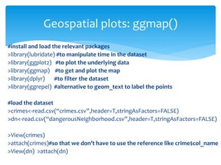
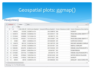
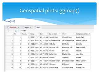
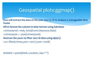
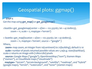
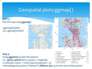
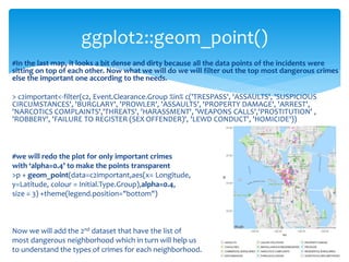
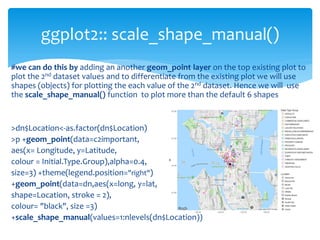
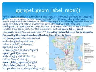
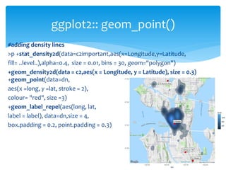
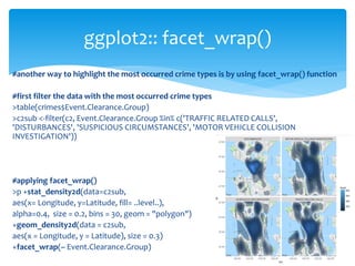
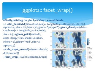
1. Geospatial plots
Using get_maps(), ggmap(), ggplot2()

2. ggmap() makes it easy to retrieve raster map tiles from popular online
mapping services like Google Maps, Stamen Maps, Open Street Map and plot
the dataset on maps using the ggplot2 framework
Includes 3 easy Steps for geospatial plots:
 First get the map using get_map(“location/coordinates”,maptype=“ ”)->p
 Second, plot the map using ggmap(p)
 Finally use ggplot2() objects like P+ geom_point(), geom_density2d() to
plot the underlying dataset.
Let’s understand this with the help of an example:
Geospatial plots: ggmap()

3. #install and load the relevant packages
>library(lubridate) #to manipulate time in the dataset
>library(ggplot2) #to plot the underlying data
>library(ggmap) #to get and plot the map
>library(dplyr) #to filter the dataset
>library(ggrepel) #alternative to geom_text to label the points
#load the dataset
>crimes<-read.csv(“crimes.csv”,header=T,stringAsFactors=FALSE)
>dn<-read.csv(“dangerousNeighborhood.csv”,header=T,stringAsFactors=FALSE)
>View(crimes)
>attach(crimes)#so that we don’t have to use the reference like crime$col_name
>View(dn) >attach(dn)
Geospatial plots: ggmap()

4. View(crimes)
Geospatial plots: ggmap()

5. View(dn)
Geospatial plots: ggmap()

6. #we will extract the data of the year 2017 to 18 to analyze a manageable time
frame
#first format the column in date format using lubridate
>crimes$ymd <-mdy_hms(Event.Clearance.Date)
>crimes$year <- year(crimes$ymd)
#extract the years to filter 2017-18 data using dplyr()
>c2<-filter(crimes,year==2017 | year==2018)
dn$label <-paste(Rank, Location, sep="-")
Geospatial plots:ggmap()

7.  STEP 1:
Get the map using get_map() or get_googlemap()
>Seattle<-get_googlemap(center = c(lon = -122.335167, lat = 47.608013),
zoom = 11, scale = 2, maptype ='terrain')
> Seattle<-get_map(location = c(lon = -122.335167, lat = 47.608013),
zoom = 11, maptype ='terrain', source = "google" )
Where,
zoom= map zoom, an integer from 10(continent) to 21(building), default is 10
scale= number of pixels returned possible values are 1,24(e.g. sizec(640X640),
scale=2 returns an image with (1280x1280) pixels
source= Google Maps ("google"), OpenStreetMap ("osm"), Stamen Maps
("stamen"), or CloudMade maps ("cloudmade")
maytype= “terrain", "terrain-background", "satellite", "roadmap", and "hybrid"
(google maps), "terrain", "watercolor", and "toner" (stamen maps)
Geospatial plots: ggmap()

8. STEP 2:
Plot the map using ggmap()
>ggmap(Seattle)
>p<- ggmap(Seattle)
Step 3:
Using ggplot2() to plot the dataset
>p + geom_point(data=c2,aes(x= Longitude,
y=Latitude, colour = Initial.Type.Group),size = 3)
+theme(legend.position="bottom") #Where size= 3 are the size of data points
Geospatial plots:ggmap()

9. #In the last map, it looks a bit dense and dirty because all the data points of the incidents were
sitting on top of each other. Now what we will do we will filter out the top most dangerous crimes
else the important one according to the needs.
> c2important<-filter(c2, Event.Clearance.Group %in% c('TRESPASS', 'ASSAULTS', 'SUSPICIOUS
CIRCUMSTANCES', 'BURGLARY', 'PROWLER', 'ASSAULTS', 'PROPERTY DAMAGE', 'ARREST',
'NARCOTICS COMPLAINTS','THREATS', 'HARASSMENT', 'WEAPONS CALLS','PROSTITUTION' ,
'ROBBERY', 'FAILURE TO REGISTER (SEX OFFENDER)', 'LEWD CONDUCT', 'HOMICIDE'))
#we will redo the plot for only important crimes
with ‘alpha=0.4’ to make the points transparent
>p + geom_point(data=c2important,aes(x= Longitude,
y=Latitude, colour = Initial.Type.Group),alpha=0.4,
size = 3) +theme(legend.position="bottom")
Now we will add the 2nd dataset that have the list of
most dangerous neighborhood which in turn will help us
to understand the types of crimes for each neighborhood.
ggplot2::geom_point()

10. #we can do this by adding an another geom_point layer on the top existing plot to
plot the 2nd dataset values and to differentiate from the existing plot we will use
shapes (objects) for plotting the each value of the 2nd dataset. Hence we will use
the scale_shape_manual() function to plot more than the default 6 shapes
>dn$Location<-as.factor(dn$Location)
>p +geom_point(data=c2important,
aes(x= Longitude, y=Latitude,
colour = Initial.Type.Group),alpha=0.4,
size=3) +theme(legend.position="right")
+geom_point(data=dn,aes(x=long, y=lat,
shape=Location, stroke = 2),
colour= "black", size =3)
+scale_shape_manual(values=1:nlevels(dn$Location))
ggplot2:: scale_shape_manual()

11. Now in previous plot we can observe that there is hardly any space left for ‘Legends’.
So to free some space for our future ‘legends’ we will simply change the shape
based neighborhood identifiers to labels. Labeling is a bit difficulty when it comes in
using two different datasets within the same plot and we might face labels
overlapping or seating on top of each other. This means we have to use some other
function than geom_text. For this example we will use geom_label_repel()
>dn$label<-paste(Rank,Location,sep="-") #creating ranked labels in the dn datasets.
#converting the shape based neighborhood identifiers to labels
>p+geom_point(data=c2important,
aes(x= Longitude, y=Latitude,
colour = Initial.Type.Group),
alpha=0.4,size= 3)
+theme(legend.position="right")
+geom_point(data=dn,
aes(x =long, y =lat, stroke = 2),
colour= "black", size =3)
+geom_label_repel(aes(long,lat,
label = label), data=dn, size = 4,
box.padding = 0.2, point.padding = 0.3)
ggrepel::geom_label_repel()

12. #Alternatively we can also plot the density of the data for each events by using
stat_density2d() function and get the same results like geom_point() function.
>p +stat_density2d(data=c2important,aes(x=Longitude,y=Latitude,
fill= ..level..),alpha=0.4,size = 0.01,
bins = 30,geom = "polygon")
+geom_point(data=dn,aes(x=long,y =lat,
stroke = 2),colour= "red", size =3)
+geom_label_repel(aes(long, lat,
label = label),data=dn,size = 4,
box.padding = 0.2, point.padding = 0.3)
#now we will add a density line to highlight
the density estimates again by
using geom_density2d() function.
ggplot2::stat_density2d()

13. #adding density lines
>p +stat_density2d(data=c2important,aes(x=Longitude,y=Latitude,
fill= ..level..),alpha=0.4, size = 0.01, bins = 30, geom="polygon")
+geom_density2d(data = c2,aes(x = Longitude, y = Latitude), size = 0.3)
+geom_point(data=dn,
aes(x =long, y =lat, stroke = 2),
colour= "red", size =3)
+geom_label_repel(aes(long, lat,
label = label), data=dn,size = 4,
box.padding = 0.2, point.padding = 0.3)
ggplot2:: geom_point()

14. #another way to highlight the most occurred crime types is by using facet_wrap() function
#first filter the data with the most occurred crime types
>table(crimes$Event.Clearance.Group)
>c2sub <-filter(c2, Event.Clearance.Group %in% c('TRAFFIC RELATED CALLS',
'DISTURBANCES', 'SUSPICIOUS CIRCUMSTANCES', 'MOTOR VEHICLE COLLISION
INVESTIGATION'))
#applying facet_wrap()
>p +stat_density2d(data=c2sub,
aes(x= Longitude, y=Latitude, fill= ..level..),
alpha=0.4, size = 0.2, bins = 30, geom = "polygon")
+geom_density2d(data = c2sub,
aes(x = Longitude, y = Latitude), size = 0.3)
+facet_wrap(~ Event.Clearance.Group)
ggplot2:: facet_wrap()

15. #Finally polishing the plot by adding the small details.
>p +stat_density2d(data=c2sub,aes(x= Longitude,y=Latitude,fill= ..level..),
alpha=0.4, size = 0.2, bins = 30, geom= "polygon")+geom_density2d(data=
c2sub,aes(x = Longitude, y = Latitude),
size = 0.3) +geom_point(data=dn,
aes(x =long, y =lat, shape=Location,
stroke = 2),colour= “red", size =2,
alpha=0.5)
+scale_shape_manual(values=1:nlevels(
dn$Location))
+facet_wrap(~ Event.Clearance.Group)
ggplot2:: facet_wrap()

16. Next: Predict the unlimited benefit using machine
learning.
Thank you