Download to read offline


![12
In order to ideally define the transmitted power PTx = 0 dBm, use a fixed output power EDFA (turn noise
off) at the output of the modulator
Receiver parameters
Rx Optical filter: SuperGaussian 2nd
order with Bo=0.33 nm
Detection
IMDD and PSBT: Photodiode: PIN with 0.60 A/W
DPSK: ideal balanced DPSK receiver including the AMZI and the balanced photodetectors
(In the Optsim tree of components you can find it under “receivers” and it is labelled “Ideal balanced
2DPSK receiver”)
TIA: ideal (transimpedance: 15kΩ, noise set to 0 pA/sqrt(Hz)
Electrical filter: low-pass Bessel 5 poles with -3 dB bandwidth Be=0.75·Rb
Channel
Noisy channel.
In this case we consider only the introduction of some ASE noise due to the chain of amplifiers and set
the OSNR at the receiver. It is suggested to use the following simulative approach
ASE noise generator added to the Tx signal with a combiner. In order to have the required OSNR [dB], set
the ASE noise generator to PTx –OSNR-10*log10(Rb) [dB(mW/THz)], where Rb [Tbit/s] is the bit-rate.
Dispersive and noisy channel
In this case, besides the ASE noise introduction, you are request to test also the presence of some
chromatic dispersion. In order to speed-up the analysis it is suggested to emulate the dispersive channel
using an ideal fiber grating (under “optical components” in the optsim library tree)
For the noise, use the ASE noise generator set as described in previous step. For the emulation of the
chromatic dispersion use an ideal fiber grating set to introduce Dacc [ps/nm].
Required analyses
Qualitative analyses (to this purpose, simulate only 211
bits, otherwise eye-diagram data files are too
large)
Verify the eye-diagrams and spectra for every modulation format](https://image.slidesharecdn.com/advancopttlcs201977makanmohammadi-180214115703/85/Advanc-optical-Telecommunication-12-320.jpg)


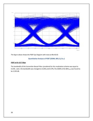


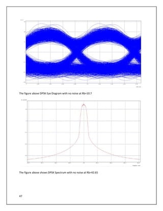


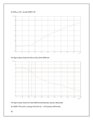


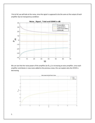
The document describes a simulation of an optical communication system using different modulation formats at bit rates of 10.7 Gbps and 42.65 Gbps. The system includes a transmitter with a laser, data source, modulator, and amplifier. A noisy channel is modeled by adding ASE noise. A receiver includes a filter, photodetector, amplifier, and error counting. Eye diagrams, spectra, and BER are analyzed for each modulation format under various channel conditions including OSNR and chromatic dispersion. The impact of increasing bandwidth for PSBT is also examined.


![[IJET-V1I2P9] Authors :Ikdeep Kaur, Harjit Singh, Anu Sheetal](https://cdn.slidesharecdn.com/ss_thumbnails/ijet-v1i2p9-150506100051-conversion-gate02-thumbnail.jpg?width=640&height=640&fit=bounds)


