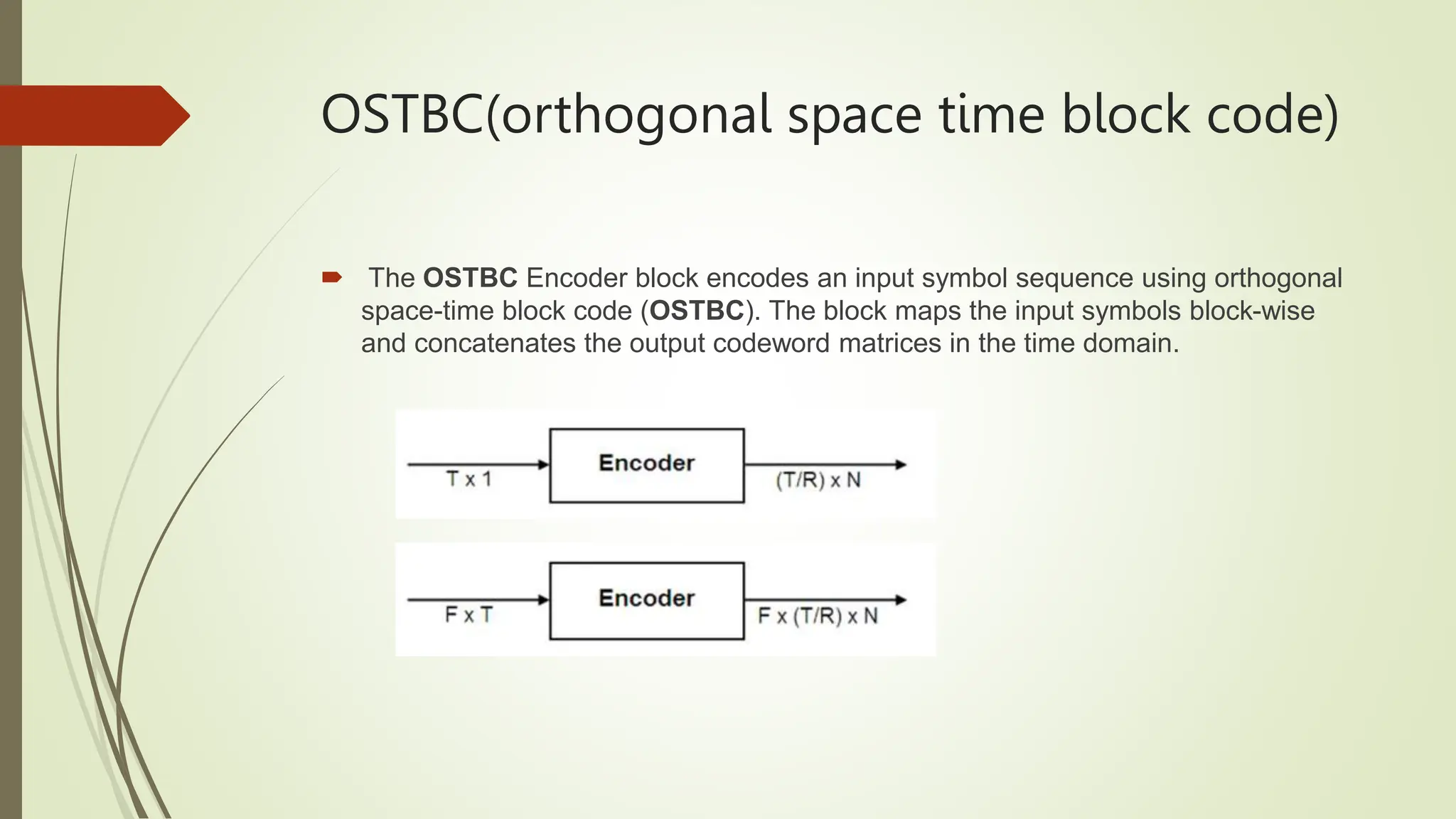
This document presents a workshop report on advanced wireless communication systems, comparing Time Division Multiple Access (TDMA) and Frequency Division Multiple Access (FDMA) technologies. It discusses the principles, advantages, and disadvantages of each method, alongside performance analysis of other communication techniques like Orthogonal Space-Time Block Codes (OSTBC), MIMO, and OFDM. Various Matlab code snippets are included to illustrate signal generation and performance metrics like bit error rate (BER) and signal-to-noise ratio (SNR) in different communication scenarios.
![grid on
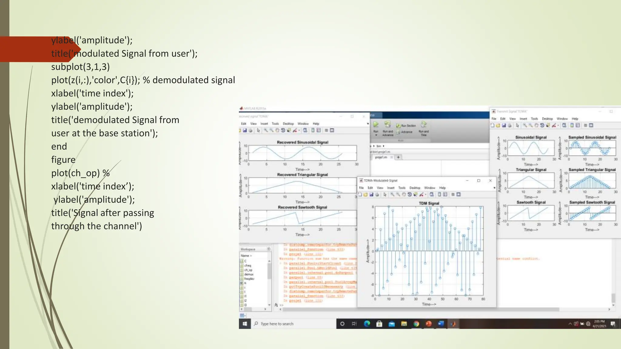
title('Sampled Sawtooth Signal');
xlabel('Time--->');
ylabel('Amplitude--->');
l1=length(sig1);
l2=length(sig2);
l3=length(sig3);
for i=1:l1
sig(1,i)=sig1(i);
sig(2,i)=sig2(i);
sig(3,i)=sig3(i);
end
tdmsig=reshape(sig,1,[]);
figure('Name','TDMA-Modulated-Signal','NumberTitle','Off');
stem(tdmsig);
grid on
title('TDM Signal');
xlabel('Time--->');
ylabel('Amplitude--->');
demux=reshape(tdmsig,3,l1);
for i=1:l1](https://image.slidesharecdn.com/workshoponadvancedwirelesscommunicationsystem-240507043521-7bff6c69/75/WORKSHOP-ON-ADVANCED-WIRELESS-COMMUNICATION-SYSTEM-pptx-11-2048.jpg)
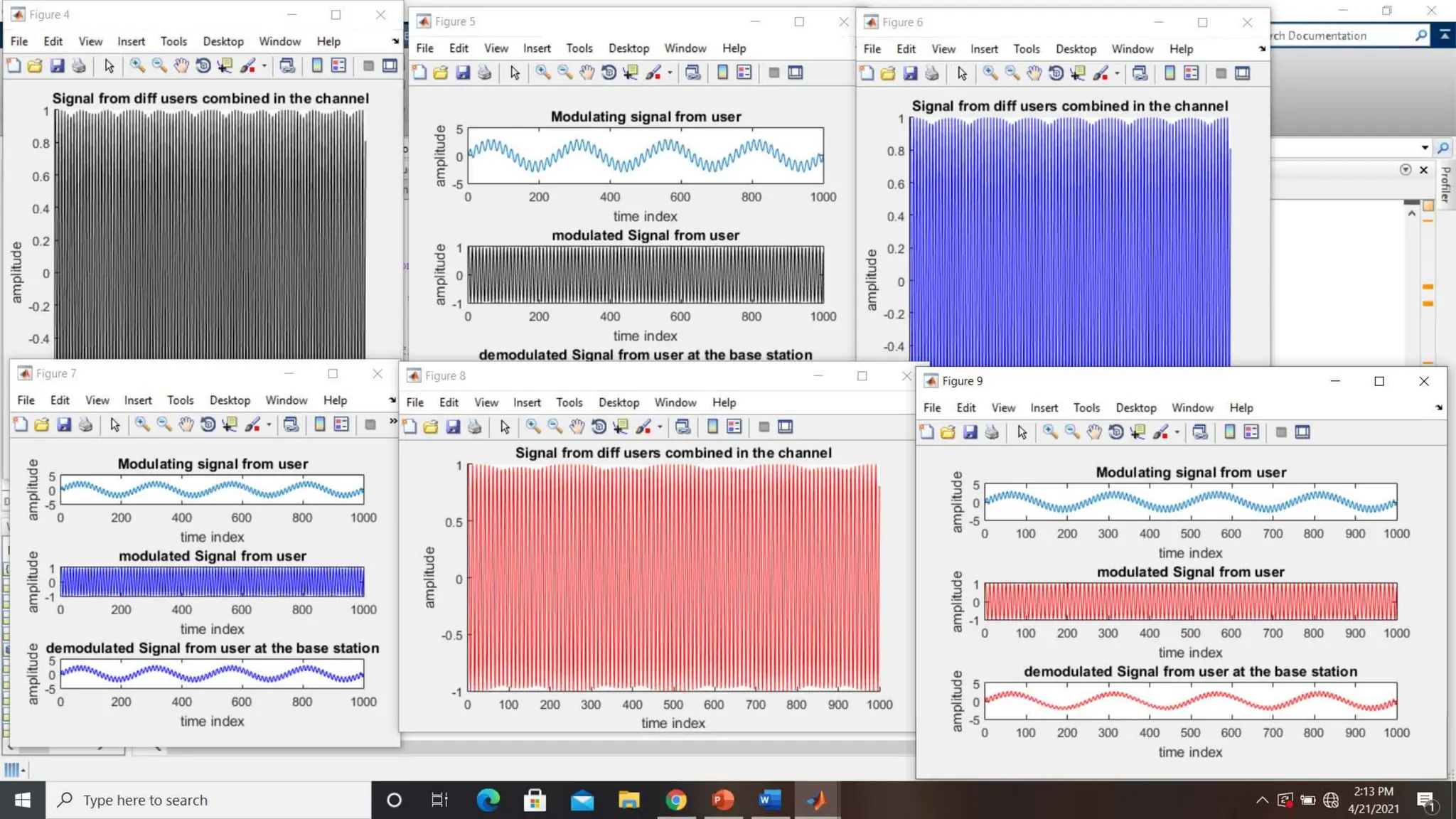
![xlabel('Time--->');
ylabel('Amplitude--->');
samples=1000;
%number of users
nos=3;
%modulating signal freq
mfreq=[60 80 100];
%carrier freq
cfreq=[1200 1800 2400];
%freq deviation
freqdev=10;
%generate modulating signal
t=linspace(0,1000,samples);
parfor i=1:nos
m(i,:)=sin(2*pi*mfreq(1,i)*t)+2*sin(pi*8*t);
end
%generate modulated signal
parfor i=1:nos
y(i,:)=fmmod(m(i,:),cfreq(1,i),10*cfreq(1,i),freqdev);
end](https://image.slidesharecdn.com/workshoponadvancedwirelesscommunicationsystem-240507043521-7bff6c69/75/WORKSHOP-ON-ADVANCED-WIRELESS-COMMUNICATION-SYSTEM-pptx-13-2048.jpg)
![CODE
clc;
snr=6;
soglia=20;
S_ML=zeros(1,4);
X_dec=zeros(1,2);
Nt=2;
Nr=2;
dec=zeros(1,2);
no_bit_sym=1;
no_it_x_SNR=10000;
iter=0;
err = 0;
tot_err_h = 0;
tot_err_ml = 0;
while tot_err_ml<soglia
iter=iter+1;
for i=1:no_it_x_SNR
Data=(2*round(rand(Nt,1))-1)/(sqrt(Nt));
H=ones(2,2);
sig = sqrt(0.5./(10.^(snr./10)));
n = sig * (randn(Nr,Nt) + j*randn(Nr,Nt));
X=[Data(1) -conj(Data(2)); Data(2) conj(Data(1))];](https://image.slidesharecdn.com/workshoponadvancedwirelesscommunicationsystem-240507043521-7bff6c69/75/WORKSHOP-ON-ADVANCED-WIRELESS-COMMUNICATION-SYSTEM-pptx-23-2048.jpg)
![R=H*X + n ;
s0=conj(H(1,1))*R(1,1)+H(1,2)*conj(R(1,2))+conj(H(2,1))*R(2,1)+H(2,2)*conj(R(2,2));
s1=conj(H(1,2))*R(1,1)-H(1,1)*conj(R(1,2))+conj(H(2,2))*R(2,1)-H(2,1)*conj(R(2,2));
S=[s0 s1];
dh = sqrt(2)*[1 -1]/2;
d11=((dh(1)-real(S(1)))^2+(imag(S(1)))^2);
d12=((dh(2)-real(S(1)))^2+(imag(S(1)))^2);
D1=[d11 d12];
for k=1:2
X1_dec(k)=((abs(dh(k)))^2)*sum(sum((abs(H)).^2)-1)+D1(k);
end
d21=((dh(1)-real(S(2)))^2+(imag(S(2)))^2);
d22=((dh(2)-real(S(2)))^2+(imag(S(2)))^2);
D2=[d21 d22];
for x=1:2
X2_dec(x)=((abs(dh(k)))^2)*sum(sum((abs(H)).^2)-1)+D2(x);
end
[scelta1, posizione1]=min(X1_dec);
[scelta2, posizione2]=min(X2_dec);
decoded=[dh(posizione1) dh(posizione2)];
err_ml = sum(round(Data')~=round(decoded));
tot_err_ml = err_ml + tot_err_ml;](https://image.slidesharecdn.com/workshoponadvancedwirelesscommunicationsystem-240507043521-7bff6c69/75/WORKSHOP-ON-ADVANCED-WIRELESS-COMMUNICATION-SYSTEM-pptx-24-2048.jpg)
![end
end
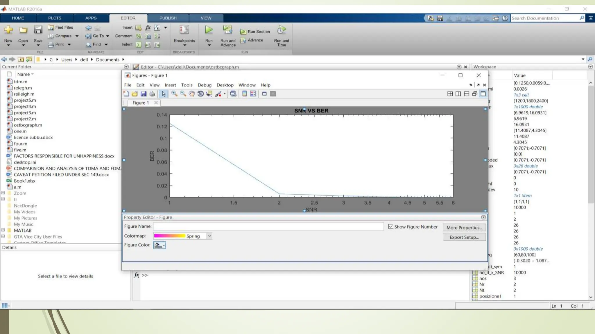
ber_ml=tot_err_ml/(no_it_x_SNR*iter*2)
PLOT
SNR = [1 2 3 4 5 6];
BER = [0.0123 0.0053 0.0025 8.5000e-04 2.0000e-04 3.4483e-05 ]
figure
plot(SNR,BER)](https://image.slidesharecdn.com/workshoponadvancedwirelesscommunicationsystem-240507043521-7bff6c69/75/WORKSHOP-ON-ADVANCED-WIRELESS-COMMUNICATION-SYSTEM-pptx-25-2048.jpg)
![code
clc;
clear all;
close all;
N=10^6;
a=randi([0,1],1,N);
b=2*a-1;
ntx=2;
snr=0:1:30;
for i=1:length(snr)
n=1/sqrt(2)*(randn(1,N)+j*randn(1,N));
h=1/sqrt(2)*(randn(ntx,N)+j*randn(ntx,N));](https://image.slidesharecdn.com/workshoponadvancedwirelesscommunicationsystem-240507043521-7bff6c69/75/WORKSHOP-ON-ADVANCED-WIRELESS-COMMUNICATION-SYSTEM-pptx-32-2048.jpg)
![code
x=[b;b];
h_tx=h.*exp(-j*angle(h));
y1=sum(h.*x,1)+(10^(-snr(i)/20)*n);
y2=sum(h_tx.*x,1)+(10^(-snr(i)/20)*n);
y_e=y1./sum(h,1);
y_b=y2./sum(h_tx,1);
d_1=real(y_e)>0;
d_2=real(y_b)>0;
err_1(i)=length(find([a-d_1]));
err_2(i)=length(find([a-d_2]));
end
n1tx=3;
for i=1:length(snr)
n3=1/sqrt(2)*(randn(1,N)+j*randn(1,N));
h3=1/sqrt(2)*(randn(n1tx,N)+j*randn(n1tx,N));](https://image.slidesharecdn.com/workshoponadvancedwirelesscommunicationsystem-240507043521-7bff6c69/75/WORKSHOP-ON-ADVANCED-WIRELESS-COMMUNICATION-SYSTEM-pptx-33-2048.jpg)
![CODE
x=[b;b];
h_tx=h.*exp(-j*angle(h));
y1=sum(h.*x,1)+(10^(-snr(i)/20)*n);
y2=sum(h_tx.*x,1)+(10^(-snr(i)/20)*n);
y_e=y1./sum(h,1);
y_b=y2./sum(h_tx,1);
d_1=real(y_e)>0;
d_2=real(y_b)>0;
err_1(i)=length(find([a-d_1]));
err_2(i)=length(find([a-d_2]));
end](https://image.slidesharecdn.com/workshoponadvancedwirelesscommunicationsystem-240507043521-7bff6c69/75/WORKSHOP-ON-ADVANCED-WIRELESS-COMMUNICATION-SYSTEM-pptx-34-2048.jpg)
![CODE
n1tx=3;
for i=1:length(snr)
n3=1/sqrt(2)*(randn(1,N)+j*randn(1,N));
h3=1/sqrt(2)*(randn(n1tx,N)+j*randn(n1tx,N));
x=[b;b;b];
h3_tx=h3.*exp(-j*angle(h3));
y3=sum(h3_tx.*x,1)+(10^(-snr(i)/20)*n3);
y3_b=y3./sum(h3_tx,1);
d_3=real(y3_b)>0;
err_3(i)=length(find([a-d_3]));
End](https://image.slidesharecdn.com/workshoponadvancedwirelesscommunicationsystem-240507043521-7bff6c69/75/WORKSHOP-ON-ADVANCED-WIRELESS-COMMUNICATION-SYSTEM-pptx-35-2048.jpg)
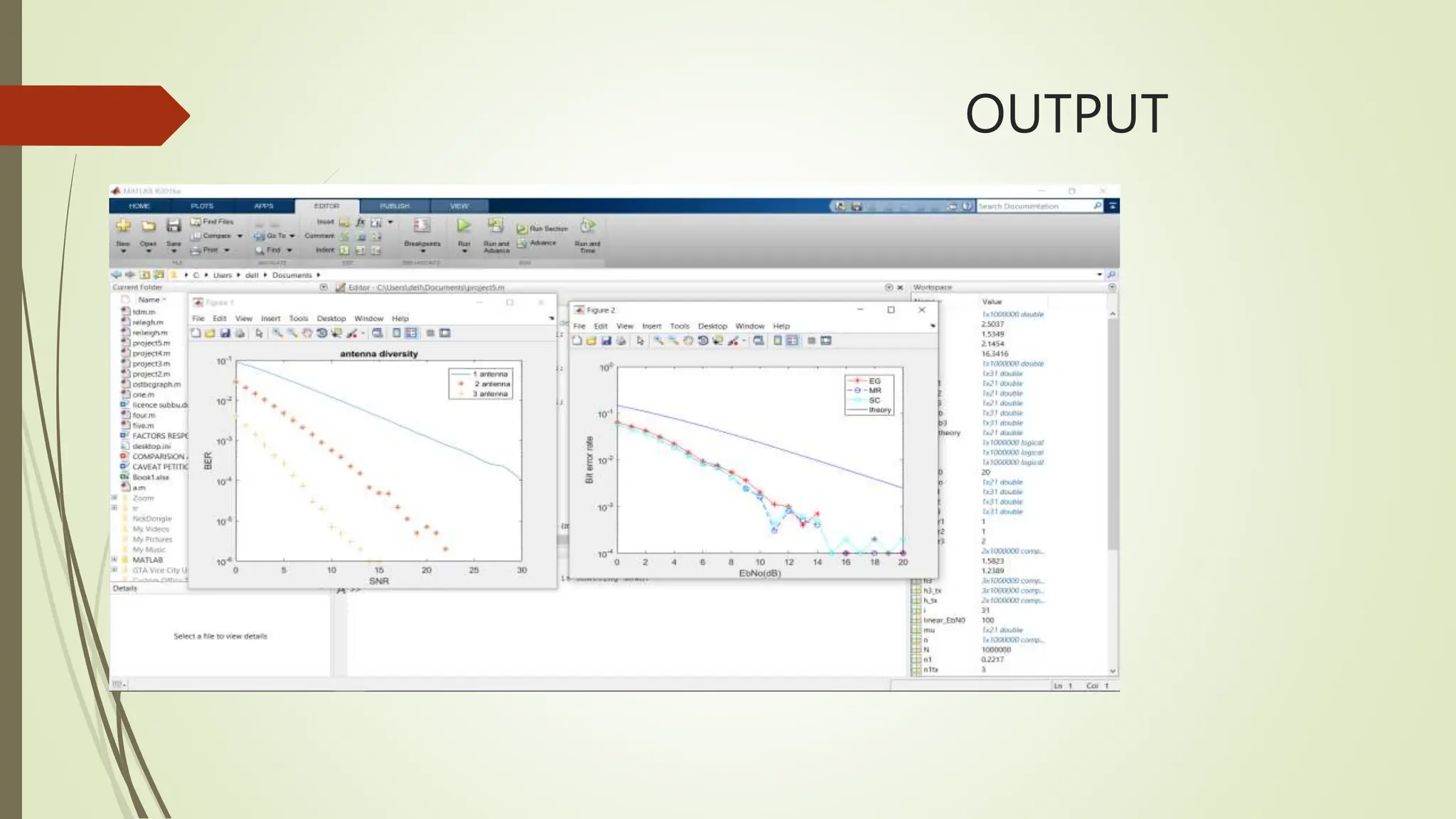
![CODE
ber=err_1/N;
ber_b=err_2/N;
ber_b3=err_3/N;
figure
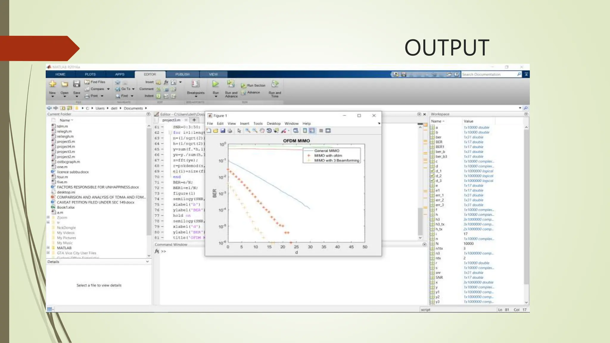
semilogy(snr,ber,'-',snr,ber_b,'*',snr,ber_b3,'+');
xlabel('SNR');
ylabel('BER');
title('Beamforming In MIMO System');
legend('General MIMO','MIMO with 2 Beamforming','MIMO with 3
Beamforming');
hold on;
N=10^4;
a=randi([0,1],1,N);
b=(2*a-1);](https://image.slidesharecdn.com/workshoponadvancedwirelesscommunicationsystem-240507043521-7bff6c69/75/WORKSHOP-ON-ADVANCED-WIRELESS-COMMUNICATION-SYSTEM-pptx-36-2048.jpg)
![CODE
c=ifft(b);
SNR=0:3:50;
for i=1:length(SNR)
n=(1/sqrt(2))*[rand(1,N)+j*rand(1,N)];
h=(1/sqrt(2))*[rand(1,N)+j*rand(1,N)];
y=sum(c.*h,1)+10^(-(SNR(i))/20)*n;
ye=y./sum(h,1);
s=fft(ye);
r=real(s)>0;
e(i)=size(find(r-a),2);
end
d=pskmod(a,4);
f=ifft(d);
SNR=0:3:50;](https://image.slidesharecdn.com/workshoponadvancedwirelesscommunicationsystem-240507043521-7bff6c69/75/WORKSHOP-ON-ADVANCED-WIRELESS-COMMUNICATION-SYSTEM-pptx-37-2048.jpg)
![Code
for i=1:length(SNR)
n=(1/sqrt(2))*[rand(1,N)+j*rand(1,N)];
h=(1/sqrt(2))*[rand(1,N)+j*rand(1,N)];
y=sum(f.*h,1)+10^(-(SNR(i))/20)*n;
ye=y./sum(h,1);
s=fft(ye);
r=pskdemod(s,4);
e1(i)=size(find(r-a),2);
end
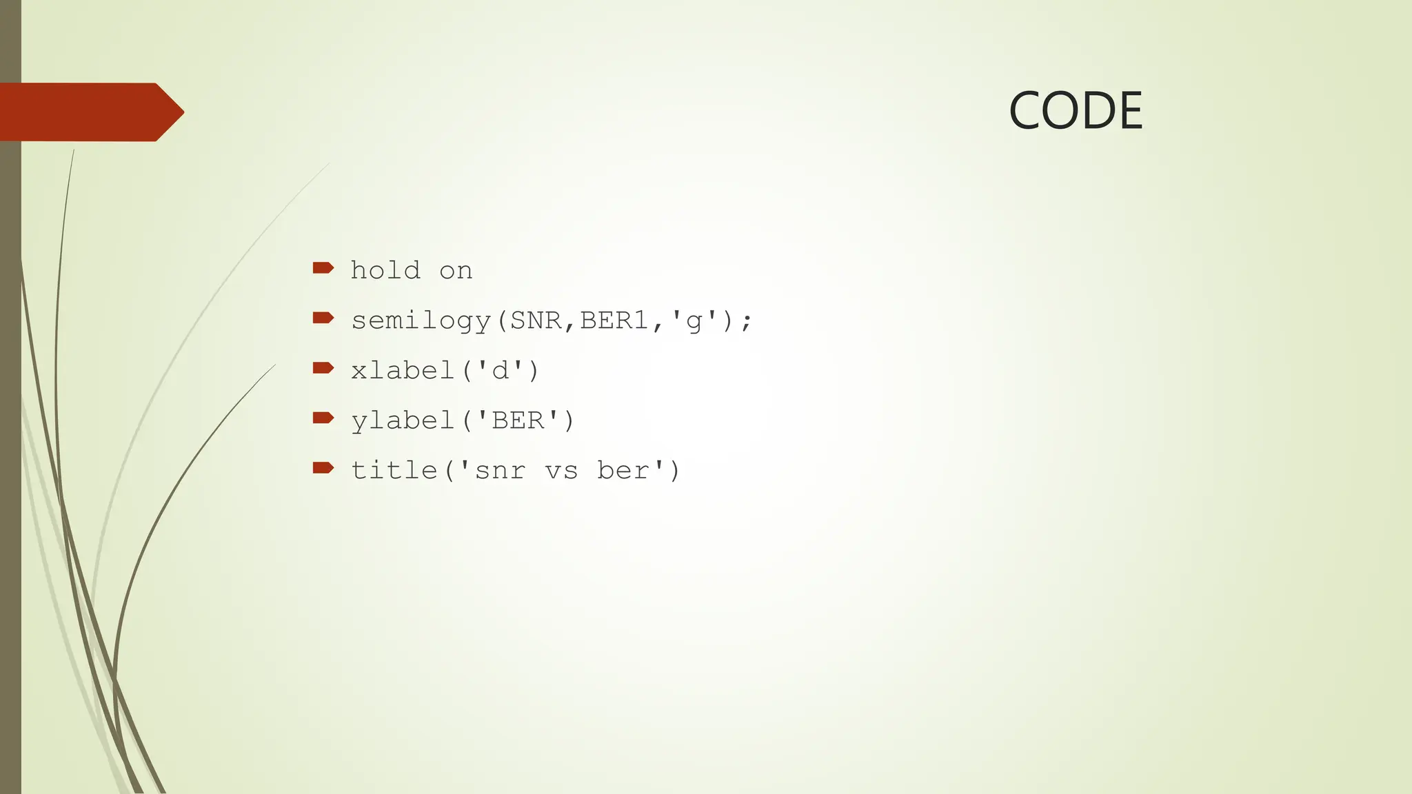
BER=e/N;
BER1=e1/N;
figure(1)
semilogy(SNR,BER,'r');
xlabel('b')
ylabel(‘BER’)](https://image.slidesharecdn.com/workshoponadvancedwirelesscommunicationsystem-240507043521-7bff6c69/75/WORKSHOP-ON-ADVANCED-WIRELESS-COMMUNICATION-SYSTEM-pptx-38-2048.jpg)
![Generation Matrix
All code words can be obtained as linear combination of basis vectors.
• The basis vectors can be designated as {𝑔1, 𝑔2, 𝑔3,….., 𝑔𝑘}
• For a linear code, there exists a k by n generator matrix such that 𝑐1∗𝑛 = 𝑚1∗𝑘 . 𝐺𝑘
∗𝑛 where c={𝑐1, 𝑐2, ….., 𝑐𝑛} and m={𝑚1, 𝑚2, ……., 𝑚𝑘}
• In this form, the code word consists of (n-k) parity check bits followed by k bits of
the message.
• The rate or efficiency for this code R= k/n
• G = [ 𝐼𝑘 P] , C = m.G = [m mP] Message part Parity part](https://image.slidesharecdn.com/workshoponadvancedwirelesscommunicationsystem-240507043521-7bff6c69/75/WORKSHOP-ON-ADVANCED-WIRELESS-COMMUNICATION-SYSTEM-pptx-44-2048.jpg)
![PARITY CHECK MATRIX (H)
When G is systematic, it is easy to determine the parity check
matrix H as: H = [𝐼𝑛−𝑘 𝑃 𝑇 ]
The parity check matrix H of a generator matrix is an (n-k)-by-
n matrix satisfying: 𝐻(𝑛−𝑘)∗𝑛𝐺𝑛∗𝑘 = 0
Then the code words should satisfy (n-k) parity check
equations 𝑐1∗𝑛𝐻𝑛∗(𝑛−𝑘) = 𝑚1∗𝑘𝐺𝑘∗𝑛𝐻𝑛∗(𝑛−𝑘) = 0](https://image.slidesharecdn.com/workshoponadvancedwirelesscommunicationsystem-240507043521-7bff6c69/75/WORKSHOP-ON-ADVANCED-WIRELESS-COMMUNICATION-SYSTEM-pptx-45-2048.jpg)
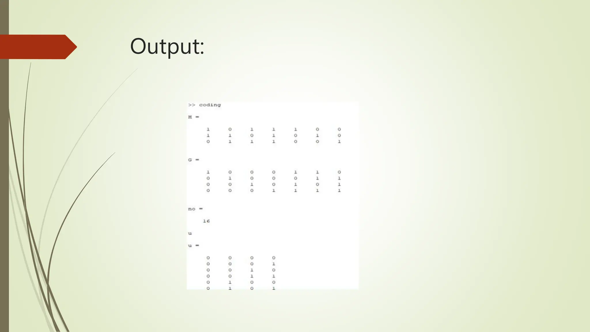
![Code:
%Given H Matrix
H = [1 0 1 1 1 0 0;
1 1 0 1 0 1 0;
0 1 1 1 0 0 1]
k = 4;
n = 7;
% Generating G Matrix
% Taking the H Matrix Transpose
P = H';
% Making a copy of H Transpose Matrix
L = P;
% Taking the last 4 rows of L and storing](https://image.slidesharecdn.com/workshoponadvancedwirelesscommunicationsystem-240507043521-7bff6c69/75/WORKSHOP-ON-ADVANCED-WIRELESS-COMMUNICATION-SYSTEM-pptx-51-2048.jpg)
![ L((5:7), : ) = [];
% Creating a Identity matrix of size K x K
I = eye(k);
% Making a 4 x 7 Matrix
G = [I L]
% Generate U data vector, denoting all information sequences
no = 2 ^ k
% Iterate through an Unit-Spaced Vector
for i = 1 : 2^k](https://image.slidesharecdn.com/workshoponadvancedwirelesscommunicationsystem-240507043521-7bff6c69/75/WORKSHOP-ON-ADVANCED-WIRELESS-COMMUNICATION-SYSTEM-pptx-52-2048.jpg)

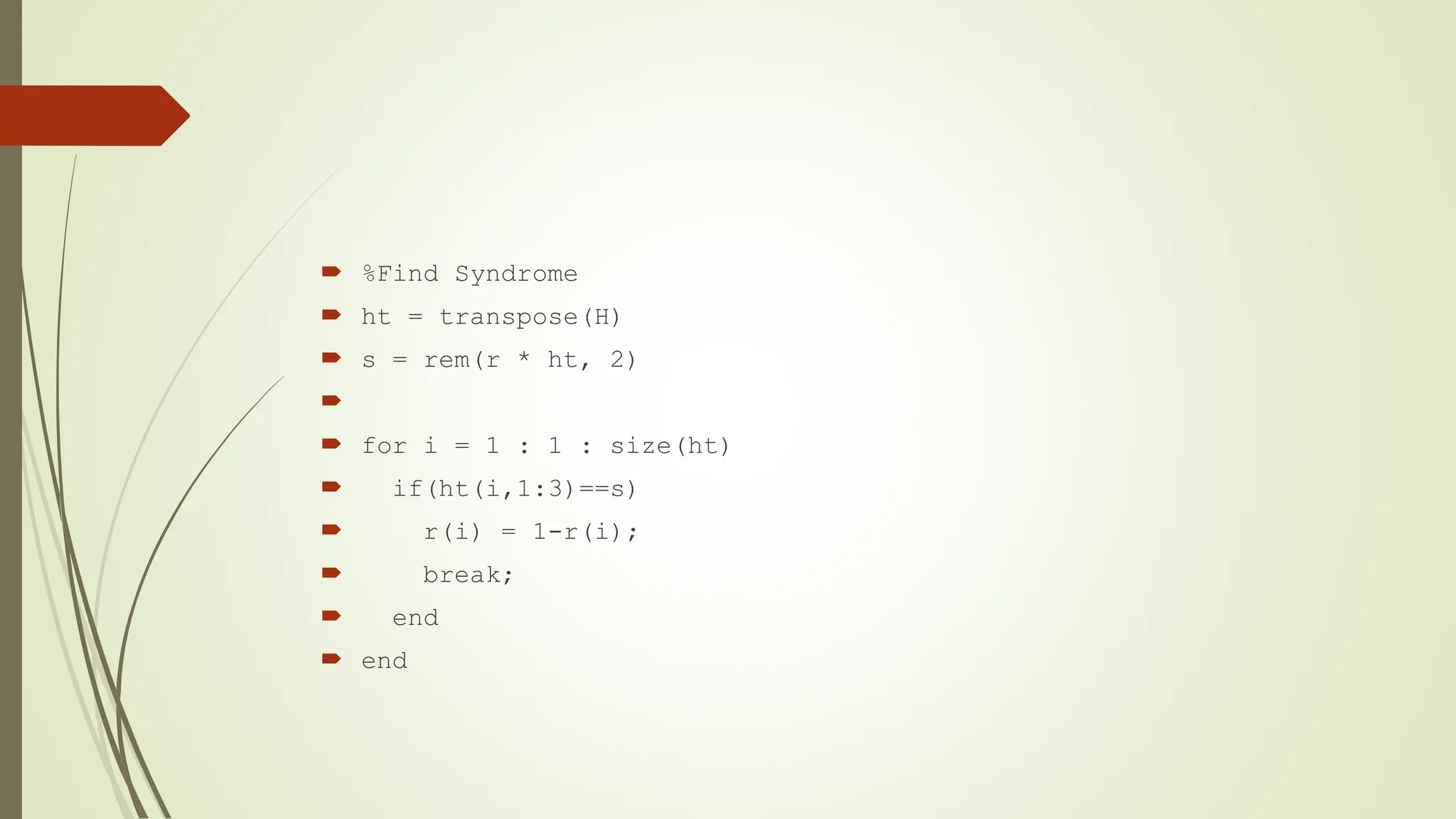
![ echo on;
u
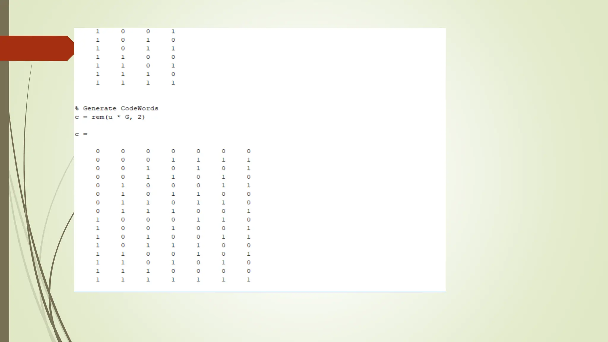
% Generate CodeWords
c = rem(u * G, 2)
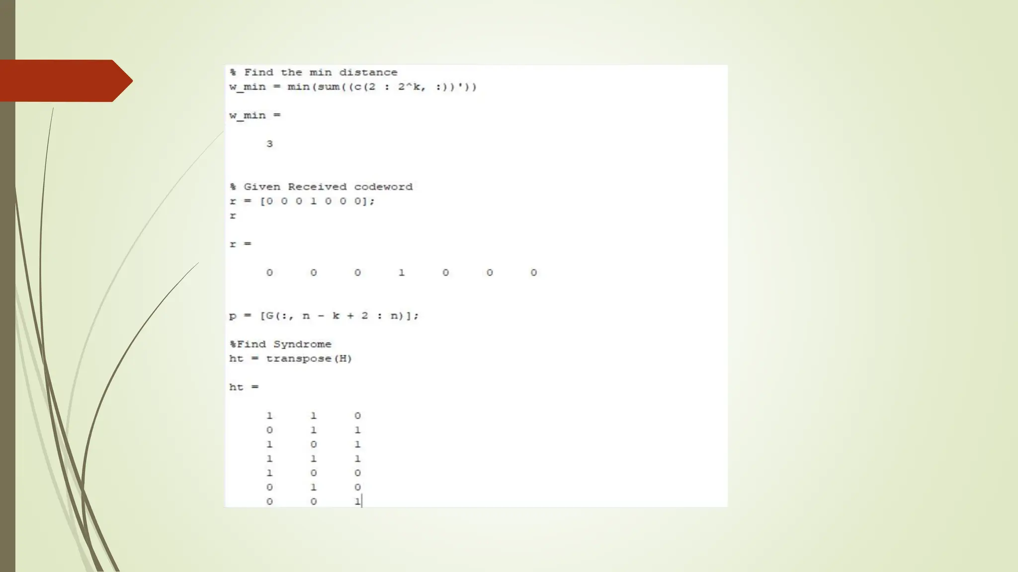
% Find the min distance
w_min = min(sum((c(2 : 2^k, :))'))
% Given Received codeword
r = [0 0 0 1 0 0 0];
r](https://image.slidesharecdn.com/workshoponadvancedwirelesscommunicationsystem-240507043521-7bff6c69/75/WORKSHOP-ON-ADVANCED-WIRELESS-COMMUNICATION-SYSTEM-pptx-54-2048.jpg)
![CODE
clc;
clear all;
close all;
N=10^6; %Length of Sequence
a=randi([0,1],1,N); %random Signal
b=2*a-1; %BPSK Modulation
ntx=2;
snr=0:1:30;
for i=1:length(snr)
n=1/sqrt(2)*(randn(1,N)+j*randn(1,N));
h=1/sqrt(2)*(randn(ntx,N)+j*randn(ntx,N));
x=[b;b];
h_tx=h.*exp(-j*angle(h));
y1=sum(h.*x,1)+(10^(-snr(i)/20)*n);
y2=sum(h_tx.*x,1)+(10^(-snr(i)/20)*n);
y_e=y1./sum(h,1);
y_b=y2./sum(h_tx,1);](https://image.slidesharecdn.com/workshoponadvancedwirelesscommunicationsystem-240507043521-7bff6c69/75/WORKSHOP-ON-ADVANCED-WIRELESS-COMMUNICATION-SYSTEM-pptx-69-2048.jpg)
![ d_2=real(y_b)>0;
err_1(i)=length(find([a-d_1]));
err_2(i)=length(find([a-d_2]));
end
n1tx=3;
for i=1:length(snr)
n3=1/sqrt(2)*(randn(1,N)+j*randn(1,N));
h3=1/sqrt(2)*(randn(n1tx,N)+j*randn(n1tx,N));
x=[b;b;b];
h3_tx=h3.*exp(-j*angle(h3));
y3=sum(h3_tx.*x,1)+(10^(-snr(i)/20)*n3);
y3_b=y3./sum(h3_tx,1);
d_3=real(y3_b)>0;
err_3(i)=length(find([a-d_3]));
end](https://image.slidesharecdn.com/workshoponadvancedwirelesscommunicationsystem-240507043521-7bff6c69/75/WORKSHOP-ON-ADVANCED-WIRELESS-COMMUNICATION-SYSTEM-pptx-70-2048.jpg)


![MILLETS [Autosaved] (1).pptx jrfjgfkjdigenej](https://cdn.slidesharecdn.com/ss_thumbnails/milletsautosaved1-240413052406-bd793011-thumbnail.jpg?width=640&height=640&fit=bounds)

![APMC [Autosaved] [Autosaved].pptx apmc duggirala](https://cdn.slidesharecdn.com/ss_thumbnails/apmcautosavedautosaved-240413053034-fd7b647f-thumbnail.jpg?width=640&height=640&fit=bounds)


![Presentation4[1].pptx food safety standards](https://cdn.slidesharecdn.com/ss_thumbnails/presentation41-240507041046-4ac8f362-thumbnail.jpg?width=640&height=640&fit=bounds)


