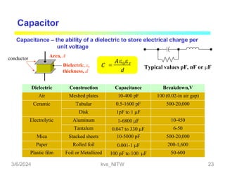
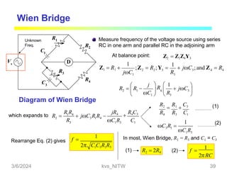
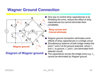
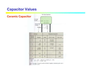
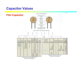
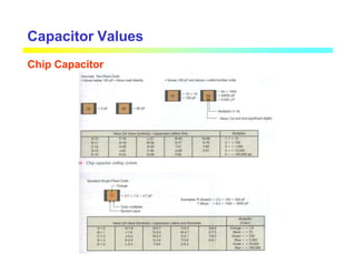
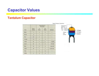
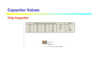
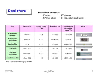
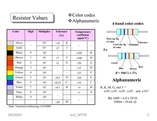
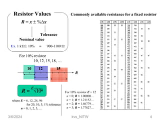
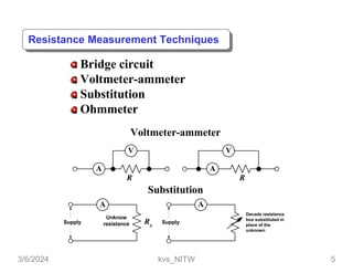
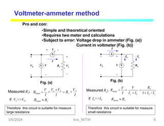
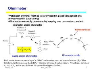
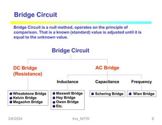
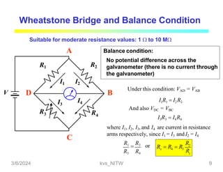
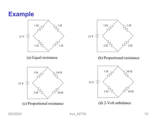
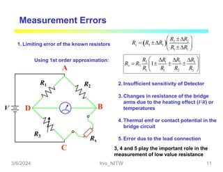
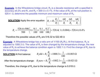
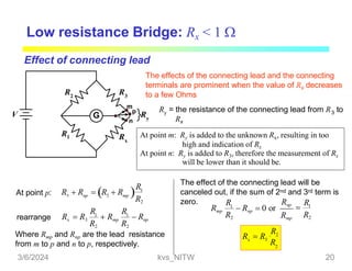
AC and DC BridgePPT for engineering students

Bridge Circuits (DC and AC)
Dr. K.V.Sridhar
Dept. of ECE,
NIT Warangal
Textbook:
-A.D. Helfrick, and W.D. Cooper, “Modern Electronic Instrumentation and Measurement
Techniques” Prentice Hall, 1994.
- D.A. Bell, “Electronic Instrumentation and Measurements”, 2nd ed., Prentice Hell, 1994.
3/6/2024 kvs_NITW 1

Type Values () Power rating
(W)
Tolerance (%) Temperature
coefficient
(ppm/°C)
picture
Wire wound
(power)
10m~3k 3~1k ±1~±10 ±30~±300
Wire wound
(precision)
10m~1M 0.1~1 ±0.005~±1 ±3~±30
Carbon film 1~1M 0.1~3 ±2~±10 ±100~±200
Metal film 100m~1M 0.1~3 ±0.5~±5 ±10~±200
Metal film
(precision)
10m~100k 0.1~1 ±0.05~±5 ±0.4~±10
Metal oxide film 100m~100k 1~10 ±2~±10 ±200~±500
Data: Transistor technology (10/2000)
Importance parameters
Value
Power rating
Tolerance
Temperature coefficient
Resistors
3/6/2024 kvs_NITW 2

Resistor Values
Color codes
Alphanumeric
Color Digit Multiplier Tolerance
(%)
Temperature
coefficient
(ppm/°C)
Silver
-
10-2
±10 K
- -
Gold 10-1
±5 J
Black 0 100 - - ±250 K
Brown 1 101 ±1 F ±100 H
Red 2 102 ±2 G ±50 G
Orange 3 103
-
- ±15 D
Yellow 4 104 - ±25 F
Green 5 105 ±0.5 D ±20 E
Blue 6 106 ±0.25 C ±10 C
Violet 7 107 ±0.1 B ±5 B
Gray 8 108
-
- ±1 A
White 9 109 -
- -
- ±20 M
Tolerance
Multiplier
Most sig. fig.
of value
Least sig. fig.
of value
Ex.
Red
Green
Blue Brown
R = 560  ± 2%
Alphanumeric
R, K, M, G, and T =
x100, x103 , x106 , x109 , and x1012
Ex. 6M8 = 6.8 x 106 
   
4 band color codes
Data: Transistor technology (10/2000)
3/6/2024 kvs_NITW 3

Commonly available resistance for a fixed resistor
Resistor Values
R = x  %x
Tolerance
Nominal value
Ex. 1 k 10%  900-1100 
For 10% resistor
10, 12, 15, 18, …
10 12 15
R
R 
E
10n
where E = 6, 12, 24, 96
for 20, 10, 5, 1% tolerance
n = 0, 1, 2, 3, …
For 10% resistor E = 12
n = 0; R = 1.00000…
n = 1; R = 1.21152…
n = 2; R = 1.46779…
n = 3; R = 1.77827…
3/6/2024 kvs_NITW 4

Bridge circuit
Voltmeter-ammeter
Substitution
Ohmmeter
Voltmeter-ammeter
A
V
R
A
V
R
x
A
Supply
Unknow
resistance
A
R Supply
Decade resistance
box substituted in
place of the
unknown
Substitution
3/6/2024 kvs_NITW 5
Resistance Measurement Techniques

Voltmeter-ammeter method
A
VS
+
-
Rx
I
IV
V V
Ix
+
-
V
VS
+
-
Rx
I
+ V -
A
A
+
-
Vx
V
-
Pro and con:
•Simple and theoretical oriented
•Requires two meter and calculations
•Subject to error: Voltage drop in ammeter (Fig. (a))
Current in voltmeter (Fig. (b))
Fig. (a)
Fig. (b)
Measured Rx:
if Vx>>VA Rmeas  Rx
V
 Rx  A
I
I I
V V V
Rmeas   x A
Therefore this circuit is suitable for measure
large resistance
x meas
Measured R : R
Rx
x V V x
1 I / I

V

V
I I  I

Rmeas  Rx
if Ix>>IV
Therefore this circuit is suitable for measure
small resistance
3/6/2024 kvs_NITW 6

Ohmmeter
•Voltmeter-ammeter method is rarely used in practical applications
(mostly used in Laboratory)
•Ohmmeter uses only one meter by keeping one parameter constant
Example: series ohmmeter
Resistance to
15k
50
Meter Infinity
resistance
Rx
be measured
Standard
resistance
Rm
Meter
Battery
VS
R1
Basic series ohmmeter consisting of a PMMC and a series-connected standard resistor (R1). When
the ohmmeter terminals are shorted (Rx = 0) meter full scale defection occurs. At half scale defection
Rx = R1 + Rm, and at zero defection the terminals are open-circuited.
Basic series ohmmeter Ohmmeter scale
Nonlinear scale
s
x 1 m
V
I
R   R  R
3/6/2024 kvs_NITW 7

Bridge Circuit is a null method, operates on the principle of
comparison. That is a known (standard) value is adjusted until it is
equal to the unknown value.
Bridge Circuit
DC Bridge
(Resistance)
AC Bridge
Inductance Capacitance Frequency
Schering Bridge Wien Bridge
Maxwell Bridge
Hay Bridge
Owen Bridge
Etc.
Wheatstone Bridge
Kelvin Bridge
Megaohm Bridge
Bridge Circuit
3/6/2024 kvs_NITW 8

Wheatstone Bridge and Balance Condition
V
R1
R3
R2
R4
I1 I2
I3
I4
Suitable for moderate resistance values: 1  to 10 M
A
B
C
D
Balance condition:
No potential difference across the
galvanometer (there is no current through
the galvanometer)
Under this condition: VAD = VAB
I1R1  I2R2
And also VDC = VBC
I3R3  I4R4
where I1, I2, I3, and I4 are current in resistance
arms respectively, since I1 = I3 and I2 = I4
R3 R4
or 2
1
R1

R2 R
x 4 3
R
R  R  R
3/6/2024 kvs_NITW 9

 
   
 
12 V
 
   
 
12 V
 
   
 
12 V
 
   
 
12 V
(a) Equal resistance (b) Proportional resistance
(c) Proportional resistance (d) 2-Volt unbalance
Example
3/6/2024 kvs_NITW 10

Measurement Errors
  2 2
3
x 3 R
R  R 
 R R
 R R 
 1 1 

V
R1
R3
R2
Rx
Using 1st order approximation:
A
B
C
D
1. Limiting error of the known resistors
3
2 1 2
R
R R R R
 
R R R
Rx  R3 1  
 
1  1 2 3 
2. Insufficient sensitivity of Detector
3. Changes in resistance of the bridge
arms due to the heating effect (I2R) or
temperatures
4. Thermal emf or contact potential in the
bridge circuit
5. Error due to the lead connection
3, 4 and 5 play the important role in the
measurement of low value resistance
3/6/2024 kvs_NITW 11

Example In the Wheatstone bridge circuit, R3 is a decade resistance with a specified in
accuracy ±0.2% and R1 and R2 = 500  ± 0.1%. If the value of R3 at the null position is
520.4  determine the possible minimum and maximum value of RX
3
2 1 2
R
R R R R
 
R R R
Rx  R3 1  
 
1  1 2 3 
SOLUTION Apply the error equation
500
x
R 
520.45001
0.1

0.1

0.2   520.4( 1 0.004)  520.40.4%

100 100 100
 
Therefore the possible values of R3 are 518.32 to 522.48 
Example A Wheatstone bridge has a ratio arm of 1/100 (R2/R1). At first balance, R3 is
adjusted to 1000.3  The value of Rx is then changed by the temperature change, the new
value of R3 to achieve the balance condition again is 1002.1  Find the change of Rx due to
the temperature change.
SOLUTION At first balance:
2
1
1000.3
1
10.003 
x
R
3
R
R old  R
2
1 100
100
1002.1
1
10.021 
x
R
3
R
After the temperature change: R new  R
Therefore, the change of Rx due to the temperature change is 0.018 
3/6/2024 kvs_NITW 12

Sensitivity of Galvanometer
A galvanometer is use to detect an unbalance condition in
Wheatstone bridge. Its sensitivity is governed by: Current sensitivity
(currents per unit defection) and internal resistance.
consider a bridge circuit under a small unbalance condition, and apply circuit
analysis to solve the current through galvanometer
Thévenin Equivalent Circuit
Thévenin Voltage (VTH)
G
B
C D
R2
R3 R4
A
I1
R1
I2
V
 I1R1  I2 R2
AD
VCD VAC V
where 1
R1  R3 2 4
and I2 
R
V V
I 
 R
Therefore
TH CD
R1 R2 
V V V


 R  R R  R 
 1 3 2 4 
3/6/2024 kvs_NITW 13

Sensitivity of Galvanometer (continued)
Thévenin Resistance (RTH)
R3
R1 R2
R4
A
B
Completed Circuit
C D
RTH  R1 // R3  R2 // R4
VTH
RTH
G
C
D
where Ig = the galvanometer current
Rg = the galvanometer resistance
g
I =
VTH
R +R
TH g
g
TH g
I 
VTH
R  R
3/6/2024 kvs_NITW 14

G C
B
R2
R3 R4
A
100 
R1
1000 
2005 
200 
5 V
(a)
C D
200  2005 
100  A 1000 
B
(b)
RTH= 734  C
D
Ig=3.34 A
G Rg= 100 
VTH
2.77 mV
(c)
D
Example 1 Figure below show the schematic diagram of a Wheatstone bridge with values of
the bridge elements. The battery voltage is 5 V and its internal resistance negligible. The
galvanometer has a current sensitivity of 10 mm/A and an internal resistance of 100 .
Calculate the deflection of the galvanometer caused by the 5- unbalance in arm BC
SOLUTION The bridge circuit is in the small unbalance condition since the value of
resistance in arm BC is 2,005 
RTH 100// 200 1000// 2005  734 
The galvanometer current
2.77 mV
g
TH g
VTH
R  R

734  100 
 3.32 A
I 
Galvanometer deflection
A
d  3.32 A
10 mm
 33.2 mm
 2.77 mV
100 1000




100  200 1000  2005
TH AD AC
V V V  5 V 
3/6/2024 kvs_NITW 15

Example 2 The galvanometer in the previous example is replaced by one with an internal
resistance of 500  and a current sensitivity of 1mm/A. Assuming that a deflection of 1 mm
can be observed on the galvanometer scale, determine if this new galvanometer is capable
of detecting the 5- unbalance in arm BC
SOLUTION Since the bridge constants have not been changed, the equivalent circuit
is again represented by a Thévenin voltage of 2.77 mV and a Thévenin resistance of
734  The new galvanometer is now connected to the output terminals, resulting a
galvanometer current.
2.77 mV
 2.24 A
g
TH g
VTH
I  
R  R 734   500 
The galvanometer deflection therefore equals 2.24 A x 1 mm/A = 2.24 mm,
indicating that this galvanometer produces a deflection that can be easily observed.
3/6/2024 kvs_NITW 16

Example 3 If all resistances in the Example 1 increase by 10 times, and we use the
galvanometer in the Example 2. Assuming that a deflection of 1 mm can be observed on the
galvanometer scale, determine if this new setting can be detected (the 50- unbalance in
arm BC)
SOLUTION
3/6/2024 kvs_NITW 17

Application of Wheatstone Bridge
Unbalance bridge
G
A
B
C D
R
R R
R+R
V
RTH = R
G
D
VTH
=V R
4R
Small unbalance
occur by the external
environment
C
Consider a bridge circuit which have identical
resistors, R in three arms, and the last arm has the
resistance of R +R. if R/R << 1
TH CD
V V V
R
4R
RTH  R
This kind of bridge circuit can be found in sensor
applications, where the resistance in one arm is
sensitive to a physical quantity such as pressure,
temperature, strain etc.
3/6/2024 kvs_NITW 18

5 k
Rv Output
signal
6 V
5 k
5 k
6
5
4
3
2
1
0
0 20 40 60 80 100 120
o
Temp ( C)
R
v
(k

(b)
Example Circuit in Figure (a) below consists of a resistor Rv which is sensitive to the
temperature change. The plot of R VS Temp. is also shown in Figure (b). Find (a) the
temperature at which the bridge is balance and (b) The output signal at Temperature of
60oC.
3 2
1
R R

5 k5 k
 5 k
R 5 k
v
(a)
SOLUTION (a) at bridge balance, we have R 
The value of Rv = 5 k corresponding to the temperature of 80oC in the given plot.
(b) at temperature of 60oC, Rv is read as 4.5 k thus R = 5 - 4.5 = 0.5 k We will
use Thévenin equivalent circuit to solve the above problem.
TH
V V
R
 6 V
0.5 k
 0.15 V
4R 45 k
It should be noted that R = 0.5 k in the problem does not satisfy the assumption R/R
<< 1, the exact calculation gives VTH = 0.158 V. However, the above calculation still gives
an acceptable solution.
4.5 k
3/6/2024 kvs_NITW 19

G
R3
R1
R2
Rx
V
m
p
n
Ry
Low resistance Bridge: Rx < 1 
terminals are prominent when the value of Rx decreases
to a few Ohms
Effect of connecting lead
The effects of the connecting lead and the connecting
At point m: Ry is added to the unknown Rx, resulting in too
high and indication of Rx
At point n: Ry is added to R3, therefore the measurement of Rx
will be lower than it should be.
y 3
R = the resistance of the connecting lead from R to
Rx
At point p:  
3 mp
np
Rx  R
R1
R2
 R  R
R R
R2 R2
Rx  R3
1
 Rmp
1
 Rnp
rearrange
Where Rmp and Rnp are the lead resistance
from m to p and n to p, respectively.
The effect of the connecting lead will be
canceled out, if the sum of 2nd and 3rd term is
zero. Rnp
Rmp
R R
R2
Rmp
1
 Rnp  0 or  1
R2
2
x
R1
3
R
R  R
3/6/2024 kvs_NITW 20

Kelvin Double Bridge: 1 to 0.00001 
Four-Terminal Resistor
Current
terminals
Voltage
terminals
Current
terminals
Voltage
terminals
Four-terminal resistors have current terminals
and potential terminals. The resistance is
defined as that between the potential
terminals, so that contact voltage drops at the
current terminals do not introduce errors.
r4
R3
R1
R2
Rx
r1
r2
r3
Ra
Rb
G
Four-Terminal Resistor and Kelvin Double Bridge
•r1 causes no effect on the balance condition.
•The effects of r2 and r3 could be minimized, if R1 >>
r2 and Ra >> r3.
•The main error comes from r4, even though this value
is very small.
3/6/2024 kvs_NITW 21

Kelvin Double Bridge: 1 to 0.00001 
G
R1
R2
p
R3
m
n
Rx
Ry
o
l
V k
I
Rb
Ra
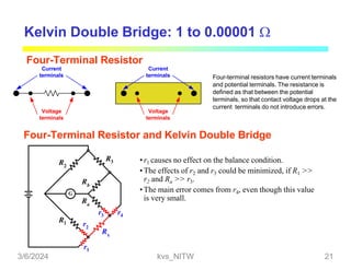
2 ratio arms: R1-R2 and Ra-Rb
the connecting lead between m and n: yoke
The balance conditions: Vlk = Vlmp or Vok = Vonp
R2
R1  R2
lk
V  V (1)
here  I[R3  Rx  (Ra  Rb ) // Ry ]
lo
V  IR
lmp 3
y
R
 
V  I R  R 
Ra  Rb  R


b
y 

(2)
Eq. (1) = (2) and rearrange: 1
RbRy
x
2 a b
R
3
R
R  R
 R1

Ra 
R 
R  R  R  R
y  2 b 

If we set R1/R2 = Ra/Rb, the second term of the right hand side will be zero, the relation
reduce to the well known relation. In summary, The resistance of the yoke has no effect
on the measurement, if the two sets of ratio arms have equal resistance ratios.
1
2
x
R
3
R
R  R
3/6/2024 kvs_NITW 22

Capacitor
Capacitance – the ability of a dielectric to store electrical charge per
unit voltage
conductor
Dielectric Construction Capacitance Breakdown,V
Air Meshed plates 10-400 pF 100 (0.02-in air gap)
Ceramic Tubular 0.5-1600 pF 500-20,000
Disk 1pF to 1 F
Electrolytic Aluminum 1-6800 F 10-450
Tantalum 0.047 to 330 F 6-50
Mica Stacked sheets 10-5000 pF 500-20,000
Paper Rolled foil 0.001-1 F 200-1,600
Plastic film Foil or Metallized 100 pF to 100 F 50-600
d
C
A 
 0 r
Area, A
Dielectric, r
thickness, d
Typical values pF, nF or F
3/6/2024 kvs_NITW 23

Inductor
A
N turns
l
l
2
A
o r N
L 
o = 410-7 H/m
r – relative permeability of core material
Ni ferrite:
Mn ferrite:
r > 200
r > 2,000
Cd
Equivalent circuit of an RF coil Distributed capacitance Cd
between turns
L Re
Air core inductor
Iron core inductor
Inductance – the ability of a conductor to produce induced voltage
when the current varies.
3/6/2024 kvs_NITW 24

Quality Factor of Inductor and Capacitor
Equivalent circuit of capacitance
Cp
Parallel equivalent circuit
Equivalent circuit of Inductance
Rp
Series equivalent circuit
Rs
Cs
Rs Xs
R2
 X 2
R2
 X 2
Rp  s s
X p  s s
Series equivalent circuit Parallel equivalent circuit
Rs
Ls
Lp
Rp
p p
s
R X 2
R 
R2
 X 2
p p
p p
s
X R2
X 
R2
 X 2
p p
3/6/2024 kvs_NITW 25

Quality Factor of Inductor and Capacitor
Inductance series circuit: Q 
Xs 
Ls
Quality factor of a coil: the ratio of reactance to resistance (frequency
dependent and circuit configuration)
Typical D ~ 10-4 – 0.1
Typical Q ~ 5 – 1000
Rs Rs
Rp
X p Lp
Inductance parallel circuit: Q 
Rp

Dissipation factor of a capacitor: the ratio of reactance to resistance
(frequency dependent and circuit configuration)
Capacitance parallel circuit:
Capacitance series circuit:
D 
X p

s s
s
X
1
Rp Cp Rp
D 
Rs
C R
3/6/2024 kvs_NITW 26

2 2 2
P P
R2
LS  P
 LP
R  L
2 2 2
P P
2
L2
RS  P
 RP
R  L
2 2
S
 L
R2
2
L2
LP  S S
LS
S
R2
R2
2
L2
RP  S S
 RS
S
S
L
Q 
R
RP
LP
Q 
S S
D C R
2 2 2
1
S P
P P
1 C R
R   R
2 2 2
1
P S
S S
1 C R
C  C
2 2 2
S S
 C R
12
C2
R2
RP  S S
RS
P P
 C R
12
C2
R2
CS  P P
C
2 2 2 P
V
I
RS LS
V
I
RP
LP
V
I RS LS
V
I
CP
RP
I
1
CP RP
D 

IRS
ILS
V

V/LP
V/RP
I

IRS
I/CS
V

VCP 
V/RP
Inductor and Capacitor
3/6/2024 kvs_NITW 27

AC bridges
• AC bridges are similar to Wheatstone bridge in which D.C. source is replaced by an
A.C. source and galvanometer with head phone/null detector.
• The resistors of bridge are replaced with combination of resistor, inductor and
capacitors (i.e. impedances).
• These bridges are used to determine the unknown capacitance/inductance of
capacitor/inductor.
• The working of these bridges is also based on Ohm’s and Kirchoff’s law.
kvs_NITW
3/6/2024 28

AC Bridge: Balance Condition
D
Z1
Z2
Z4
Z3
A C
D
B
I1 I2
all four arms are considered as impedance
(frequency dependent components)
The detector is an ac responding device:
headphone, ac meter
Source: an ac voltage at desired frequency
General Form of the ac Bridge
Complex Form:
Z1, Z2, Z3 and Z4 are the impedance of bridge arms
At balance point: E = E or I Z = I Z
1 2
2 4
BA BC 1 1 2 2
V V
and I =
Z1 + Z3 Z + Z
I =
V
Z1Z4 = Z2Z3
Z1Z4 1  4 =Z2Z3 2  3 
Polar Form:
Magnitude balance:
Phase balance:
Z1Z4 =Z2Z3
1  4 =2  3
3/6/2024 kvs_NITW 29

Example The impedance of the basic ac bridge are given as follows:
Z 100  80o
(inductive impedance)
1
Z2  250  (pure resistance)
Determine the constants of the unknown arm.
SOLUTION The first condition for bridge balance requires that
Z  400 30o
 (inductive impedance)
3
Z4  unknown

Z2Z3
4
1
Z 100

250 400
1,000 
Z
The second condition for bridge balance requires that the sum of the phase angles of
opposite arms be equal, therefore
o
4 =2  3  1  0  30 80  50
o
Hence the unknown impedance Z4 can be written in polar form as
Z4 1,000    50
Indicating that we are dealing with a capacitive element, possibly consisting of a
series combination of at resistor and a capacitor.
3/6/2024 kvs_NITW 30

Example an ac bridge is in balance with the following constants: arm AB, R = 200 
in series with L = 15.9 mH R; arm BC, R = 300  in series with C = 0.265 F; arm CD,
unknown; arm DA, = 450 . The oscillator frequency is 1 kHz. Find the constants of
arm CD.
SOLUTION
This result indicates that Z4 is a pure inductance with an inductive reactance of 150 
at at frequency of 1kHz. Since the inductive reactance XL = 2fL, we solve for L and
obtain L = 23.9 mH
D
Z1
Z2
Z4
Z3
A
D
The general equation for bridge balance states that
C
B
I1
I2
V
Z1  R  jL  200 j100 
Z  R 1/ jC  300  j600 
2
Z3  R  450 
Z4  unknown
Z1Z4 = Z2Z3
Z1 (300  j600)
=
Z2Z3

450(200  j100)
 j150 
4
Z
3/6/2024 kvs_NITW 31

Comparison Bridge: Capacitance
Measure an unknown inductance or
capacitance by comparing with it with a known
inductance or capacitance.
At balance point: Z1Zx = Z2Z3
1 1 2
where Z =R ;Z = R2; and Z3  R3 
3
1
jC
2 3
1 1
jC jC
  
 R R 


R1  Rx  
x  

3 

2 3
1
x
R R
R
Diagram of Capacitance
Comparison Bridge
Separation of the real and imaginary terms yields: R 
2
x
R1
3
R
C  C
and
Frequency independent
To satisfy both balance conditions, the bridge must contain two variable
elements in its configuration.
D
R2
R1
Rx
Unknown
capacitance
C3
R3 Cx
Vs
3/6/2024 kvs_NITW 32

Comparison Bridge: Inductance
Measure an unknown inductance or
capacitance by comparing with it with a known
inductance or capacitance.
1 1 2
where Z =R ;Z = R2; and Z3  R3  jL3
R1 Rx  jLx  R2 RS  jLS 
2 3
1
x
R R
R
Diagram of Inductance
Comparison Bridge
Separation of the real and imaginary terms yields: R  2
1
R
R
Lx  L3
and
To satisfy both balance conditions, the bridge must contain two variable
elements in its configuration.
D
R2
R1
L3
Rx
Lx
Unknown
inductance
R3
Vs
3/6/2024 kvs_NITW 33

Maxwell Bridge
Measure an unknown inductance in terms of
a known capacitance
D
R2
R1
C1
R3
Rx
V
Lx
Unknown
inductance
At balance point: Zx = Z2Z3Y1
2
where Z 2 3 3 1 1
1
R
= R ; Z  R ; and Y =
1
 jC
x
R
x x 2 3  1 
 1 
Z = R  jL  R R
 1
 jC

2 3
1
x
R R
R
Diagram of Maxwell Bridge
Separation of the real and imaginary terms yields: R  Lx  R2R3C1
and
Suitable for Medium Q coil (1-10), impractical for high Q coil: since R1 will be very
large.
3/6/2024 kvs_NITW 34

Hay Bridge
Similar to Maxwell bridge: but R1 series with C1
Diagram of Hay Bridge
V
1 1
1
j
C
where Z = R  ; Z2  R2; and Z3  R3
x 2 3

R 
1 
R  jL  R R
 1 x
jC 
 1 
which expands to
D
R2
R1
C1
R3
Rx
Lx
Unknown
inductance
L jR
C1 C1
R1Rx  x
 x
 jLx R1  R2R3
L
C1
R1Rx  x
 R2R3 (1)
x 1
1
Rx
C
 L R (2)
Solve the above equations simultaneously
3/6/2024 kvs_NITW 35

Hay Bridge: continues
2 2 2
1 1
x
R2R3C1
L 
1 C R
2 2 2
1 1
2
C2
R R R
Rx  1 1 2 3
1 C R
Lx
Rx
Z
L
R1
Z
C

C1
and
Phasor diagram of arm 4 and 1
L
tan
x

XL

Lx
 Q
1 1
C
tan
R C R
R R

XC 1

1 1
L C
tan
C R
 tan or Q 
1
Thus, Lx can be rewritten as
R2R3C1
x
L 
1 (1/Q2
)
For high Q coil (> 10), the term (1/Q)2 can be neglected Lx  R2R3C1
3/6/2024 kvs_NITW 36

Schering Bridge
Used extensively for the measurement of capacitance
and the quality of capacitor in term of D
D
R2
R1
C1
C3
Rx
Cx
Unknown
capacitance
V
Diagram of Schering Bridge
At balance point: x 2 3 1
where Z2 = R2; Z3  1
3 1
Z = Z Z Y
1
R
jC
; and Y =
1
 jC
x
Rx
j

C C R
  j  1
 R2  
 x  1

 jC1 

which expands to
x 3 3 1
x
R 
C C C R
j

R2C1 jR2

1
3
x
C
2
C
Separation of the real and imaginary terms yields: R  R
2
x
R1
3
R
and C  C
3/6/2024 kvs_NITW 37

Schering Bridge: continues
Dissipation factor of a series RC circuit: x x
x
X
D 
Rx
R C
Dissipation factor tells us about the quality of a capacitor, how close the
phase angle of the capacitor is to the ideal value of 90o
D RxCx R1C1
For Schering Bridge:
For Schering Bridge, R1 is a fixed value, the dial of C1 can be calibrated directly in D
at one particular frequency
3/6/2024 kvs_NITW 38

Wien Bridge
D
Measure frequency of the voltage source using series
R2 RC in one arm and parallel RC in the adjoining arm
R1
1
C3
R4
R3
Vs
Diagram of Wien Bridge
At balance point: Z2  Z1Z4Y3
j
 jC

3 
R

R
 1
R 

R  4 
2  1
C 
 1   3 
Unknown
Freq.
C
which expands to
jR4

R4C3
1 4
2 3 1 4
3 1 3 1
R R
R   jC R R 
R C R C
R2

R1

C3
R4 R3 C1
3 1
1 3
1
C R 
C R
(1)
(2)
f 
1
2 C1C3R1R3
Rearrange Eq. (2) gives
In most, Wien Bridge, R1 = R3 and C1 = C3
R2  2R4
2RC
f 
1
(1) (2)
4
4
3
2 2 3 3
1
Z1  R1 
1
R
;Z  R ;Y 
1
 jC ; and Z  R
jC
3/6/2024 kvs_NITW 39

Wagner Ground Connection
D
R2
R1
C3
Rx
1
2
R3 Cx
Rw
Cw
C1
C2
D
A B
C
Diagram of Wagner ground
Wagner ground connection eliminates some
effects of stray capacitances in a bridge circuit
Simultaneous balance of both bridge makes the
point 1 and 2 at the ground potential. (short C1
and C2 to ground, C4 and C5 are eliminated from
detector circuit)
The capacitance across the bridge arms e.g. C6
cannot be eliminated by Wagner ground.
Wagner ground
Stray across arm
Cannot eliminate
One way to control stray capacitances is by
Shielding the arms, reduce the effect of stray
capacitances but cannot eliminate them
completely.
C4
C5
C6
3/6/2024 kvs_NITW 40

Capacitor Values
Ceramic Capacitor

Capacitor Values
Film Capacitor

Capacitor Values
Chip Capacitor

Capacitor Values
Tantalum Capacitor

AC and DC BridgePPT for engineering students

More Related Content

What's hot

Similar to AC and DC BridgePPT for engineering students

More from National Institute of Technolgy(REC) warangal

Recently uploaded

AC and DC BridgePPT for engineering students