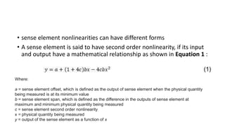
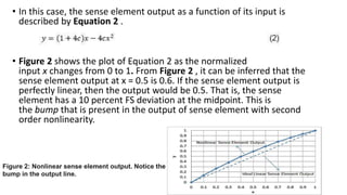
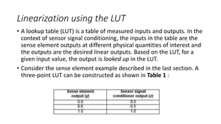
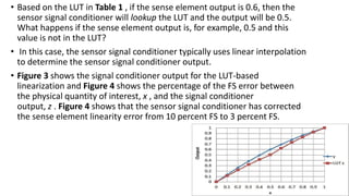
• sense element nonlinearities can have different forms
• A sense element is said to have second order nonlinearity, if its input
and output have a mathematical relationship as shown in Equation 1 :
Where:
a = sense element offset, which is defined as the output of sense element when the physical quantity
being measured is at its minimum value
b = sense element span, which is defined as the difference in the outputs of sense element at
maximum and minimum physical quantity being measured
c = sense element second order nonlinearity
x = physical quantity being measured
y = output of the sense element as a function of x
• For example, consider a nonlinear sense element with the following
example parameters:
• x is between 0 and 1. That is, the physical quantity has been
normalized and so has no units
• a = 0
• b = 1
• c = 10 percent full scale (FS), where FS = b; in other words, the sense
element has 10 percent nonlinearity.
• In this case, the sense element output as a function of its input is
described by Equation 2 .
• Figure 2 shows the plot of Equation 2 as the normalized
input x changes from 0 to 1. From Figure 2 , it can be inferred that the
sense element output at x = 0.5 is 0.6. If the sense element output is
perfectly linear, then the output would be 0.5. That is, the sense
element has a 10 percent FS deviation at the midpoint. This is
the bump that is present in the output of sense element with second
order nonlinearity.
Figure 2: Nonlinear sense element output. Notice the
bump in the output line.
Linearizing the sense element output
• The goal of linearization of the sense element output is to make the
nonlinear line linear.
• we discuss two common approaches that are used in sensor signal
conditioners. using analog circuits as in the PGA309, or using digital
logic or firmware as in the PGA900.
Linearization using the LUT
• A lookup table (LUT) is a table of measured inputs and outputs. In the
context of sensor signal conditioning, the inputs in the table are the
sense element outputs at different physical quantities of interest and
the outputs are the desired linear outputs. Based on the LUT, for a
given input value, the output is looked up in the LUT.
• Consider the sense element example described in the last section. A
three-point LUT can be constructed as shown in Table 1 :
• Based on the LUT in Table 1 , if the sense element output is 0.6, then the
sensor signal conditioner will lookup the LUT and the output will be 0.5.
What happens if the sense element output is, for example, 0.5 and this
value is not in the LUT?
• In this case, the sensor signal conditioner typically uses linear interpolation
to determine the sensor signal conditioner output.
• Figure 3 shows the signal conditioner output for the LUT-based
linearization and Figure 4 shows the percentage of the FS error between
the physical quantity of interest, x , and the signal conditioner
output, z . Figure 4 shows that the sensor signal conditioner has corrected
the sense element linearity error from 10 percent FS to 3 percent FS.
Linearization using polynomials
• We next consider the linearization using polynomials. Specifically, we use a three-
coefficient polynomial (similar to using a three-point LUT), or a second-order
polynomial given by Equation 3:
• Where h , g and n are the polynomial coefficients, y is the output of the sense
element, and z is the output of the sensor signal conditioner.
• Consider the sense element example we described earlier. Using Equation
2 , Equation 3 can be rewritten as Equation 4 :
• The goal of linearization is to remove the dependence of the signal conditioner
output on x2 . This can be achieved by choosing polynomial coefficients h , g and n so
that the resultant coefficients of are eliminated or small.
•
• Using algebraic manipulations, the three polynomial coefficients to
minimize resultant coefficients of x2 can be evaluated to:
• The sensor signal conditioner uses the above coefficient’s values and
calculates the linearized output using Equation 3 .
• Figure 5 shows the signal conditioner output for polynomial-based
linearization, while Figure 6 shows the percentage of FS error
between the physical quantity of interest, x, and the signal
conditioner output, z . Figure 6 shows that the sensor signal
conditioner has corrected the sense element linearity error from 10
percent of FS to 1.5 percent of FS.
Note that the nonlinearity error can be further reduced by
choosing more numbers of coefficients in the polynomial –
or by choosing higher order polynomials.
Figure 6: A percentage of FS error with linearization
using polynomials.
Figure 5: Linearization using polynomials.
lut based linearization.pptx

lut based linearization.pptx

  • 2.
    • sense elementnonlinearities can have different forms • A sense element is said to have second order nonlinearity, if its input and output have a mathematical relationship as shown in Equation 1 : Where: a = sense element offset, which is defined as the output of sense element when the physical quantity being measured is at its minimum value b = sense element span, which is defined as the difference in the outputs of sense element at maximum and minimum physical quantity being measured c = sense element second order nonlinearity x = physical quantity being measured y = output of the sense element as a function of x
  • 3.
    • For example,consider a nonlinear sense element with the following example parameters: • x is between 0 and 1. That is, the physical quantity has been normalized and so has no units • a = 0 • b = 1 • c = 10 percent full scale (FS), where FS = b; in other words, the sense element has 10 percent nonlinearity.
  • 4.
    • In thiscase, the sense element output as a function of its input is described by Equation 2 . • Figure 2 shows the plot of Equation 2 as the normalized input x changes from 0 to 1. From Figure 2 , it can be inferred that the sense element output at x = 0.5 is 0.6. If the sense element output is perfectly linear, then the output would be 0.5. That is, the sense element has a 10 percent FS deviation at the midpoint. This is the bump that is present in the output of sense element with second order nonlinearity. Figure 2: Nonlinear sense element output. Notice the bump in the output line.
  • 5.
    Linearizing the senseelement output • The goal of linearization of the sense element output is to make the nonlinear line linear. • we discuss two common approaches that are used in sensor signal conditioners. using analog circuits as in the PGA309, or using digital logic or firmware as in the PGA900.
  • 6.
    Linearization using theLUT • A lookup table (LUT) is a table of measured inputs and outputs. In the context of sensor signal conditioning, the inputs in the table are the sense element outputs at different physical quantities of interest and the outputs are the desired linear outputs. Based on the LUT, for a given input value, the output is looked up in the LUT. • Consider the sense element example described in the last section. A three-point LUT can be constructed as shown in Table 1 :
  • 7.
    • Based onthe LUT in Table 1 , if the sense element output is 0.6, then the sensor signal conditioner will lookup the LUT and the output will be 0.5. What happens if the sense element output is, for example, 0.5 and this value is not in the LUT? • In this case, the sensor signal conditioner typically uses linear interpolation to determine the sensor signal conditioner output. • Figure 3 shows the signal conditioner output for the LUT-based linearization and Figure 4 shows the percentage of the FS error between the physical quantity of interest, x , and the signal conditioner output, z . Figure 4 shows that the sensor signal conditioner has corrected the sense element linearity error from 10 percent FS to 3 percent FS.
  • 8.
    Linearization using polynomials •We next consider the linearization using polynomials. Specifically, we use a three- coefficient polynomial (similar to using a three-point LUT), or a second-order polynomial given by Equation 3: • Where h , g and n are the polynomial coefficients, y is the output of the sense element, and z is the output of the sensor signal conditioner. • Consider the sense element example we described earlier. Using Equation 2 , Equation 3 can be rewritten as Equation 4 : • The goal of linearization is to remove the dependence of the signal conditioner output on x2 . This can be achieved by choosing polynomial coefficients h , g and n so that the resultant coefficients of are eliminated or small. •
  • 9.
    • Using algebraicmanipulations, the three polynomial coefficients to minimize resultant coefficients of x2 can be evaluated to: • The sensor signal conditioner uses the above coefficient’s values and calculates the linearized output using Equation 3 . • Figure 5 shows the signal conditioner output for polynomial-based linearization, while Figure 6 shows the percentage of FS error between the physical quantity of interest, x, and the signal conditioner output, z . Figure 6 shows that the sensor signal conditioner has corrected the sense element linearity error from 10 percent of FS to 1.5 percent of FS.
  • 10.
    Note that thenonlinearity error can be further reduced by choosing more numbers of coefficients in the polynomial – or by choosing higher order polynomials. Figure 6: A percentage of FS error with linearization using polynomials. Figure 5: Linearization using polynomials.