The document discusses the importance of detecting and repairing GPS cycle slips to ensure accurate positioning using various signal combinations. It outlines different techniques for detecting and repairing cycle slips, including graphical detection and statistical tests like z-scores and quartiles. The research demonstrates how various test quantities influence detection capabilities and highlights the superior performance of statistical approaches over graphical methods.

1. International
OPEN ACCESS Journal
Of Modern Engineering Research (IJMER)
| IJMER | ISSN: 2249–6645 | www.ijmer.com | Vol. 4 | Iss.11| Nov. 2014 | 1|
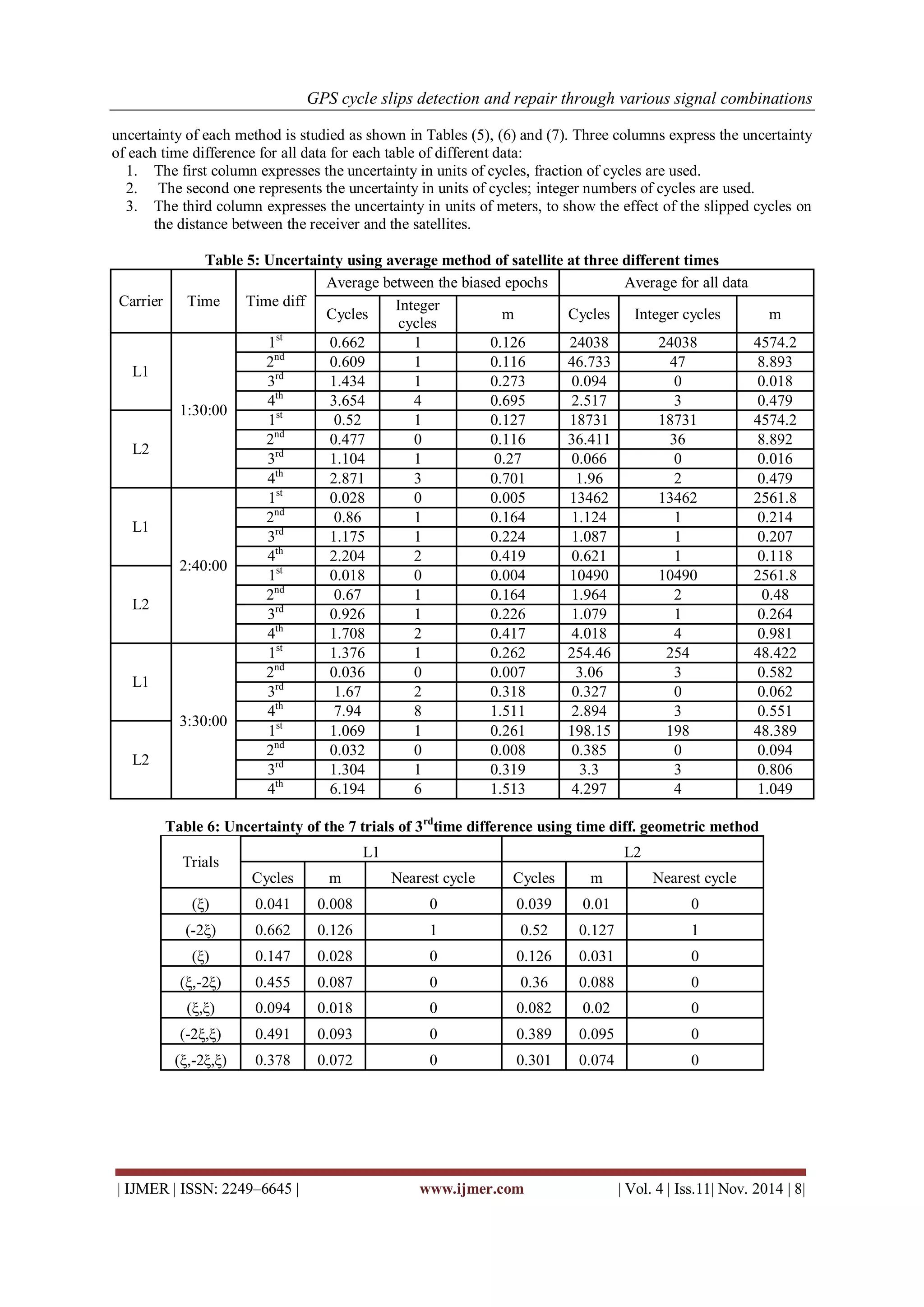
GPS cycle slips detection and repair through various signal combinations
M. E. El-Tokhey1, T. F. Sorour 2, A. E. Ragheb3, M. O. Moursy4 1Professor of surveying and geodesy, Public Works department, Faculty of Engineering, Ain Shams University, Egypt 2Associate Professor of surveying and geodesy, Public Works department, Faculty of Engineering, Ain Shams University, Egypt 3Assistant Professor of surveying and geodesy, Public Works department, Faculty of Engineering, Ain Shams University, Egypt 4Instructor of surveying and geodesy, Public Works department, Faculty of Engineering, Ain Shams University, Egypt
I. Introduction
It is well known that there are two fundamental types of GPS observations which are the pseudo-range (code) observations and the carrier phase observations [1]. The pseudo-range observations are immune against cycle slips. On the other hand, carrier phase measurements are much more accurate than pseudo-range observations. The accuracy of pseudo-range measurement is in the meter (or sub-meter) level, whereas in the centimeter level for carrier phase measurements. So, cycle slips must be detected and then repaired for the carrier phase observations to determine accurate position [2]. Cycle slips detection is the process of checking the occurrence of the cycle slips and then discovering the specific epoch which the slipped cycles took place. Cycle slips repair process takes place after detecting the time of occurrence when the cycle slips took place at a certain epoch [3]. Cycle slip repair involves the determination of the integer number of slipped cycles, and then removing these slipped cycles from the data (i.e.; correcting all subsequent phase observations for this satellite and this carrier by a fixed amount which is the slipped cycles [4]. Many researches were concerned with the handling of cycle slips, leading to many different techniques. Such developed techniques are different in their mathematical basis, required pre-requisite data, type of used GPS receiver and possibility of application in real-time. In this paper, many different techniques of cycle slip detection and repairing are tested. Such techniques are different in the nature of the used data and the used test quantity. Also, some new approaches will be tried to increase the quality of the detection and repairing processes.
II. Different used test quantities in detecting and repairing GPS cycle slips
Single series of phase observations cannot detect and repair cycle slips alone, but they should be combined with other quantities and the behavior of this combination should be analyzed. This combination is called test quantity which should have a smooth behavior [5]. In other words, when plotting the test quantity versus time, a smooth curve is created. If a sudden jump (discontinuity) appears in that curve, this will indicate a cycle slip at this epoch. There are some factors should be taken into consideration when choosing the test quantity, which are [6]:
1. Type of receiver used (single or dual frequency)
2. Kind of observation mode (static or kinematic)
Abstract: GPS Cycle slips affect the measured spatial distance between the satellite and the receiver, thus affecting the accuracy of the derived 3D coordinates of any ground station. Therefore, cycle slips must be detected and repaired before performing any data processing. The objectives of this research are to detect the Cycle slips by using various types of GPS signal combinations with graphical and statistical tests techniques, and to repair cycle slips by using average and time difference geometry techniques. Results of detection process show that the graphical detection can be used as a primary detection technique whereas the statistical approaches of detection are proved to be superior. On the other hand, results of repairing process show that any trial can be used for such process except for the 1st and 2nd time differences averaging all data as they give very low accuracy of the cycle slip fixation.
Key Words: Cycle slips detection and repair, Quartiles, Time difference, Z-score.

2. GPS cycle slips detection and repair through various signal combinations
| IJMER | ISSN: 2249–6645 | www.ijmer.com | Vol. 4 | Iss.11| Nov. 2014 | 2|
3. Type of positioning mode (single point or relative positioning)
4. The availability of some information such as satellite and station coordinates
On the other hand, different types of test quantities are available based on:
 Linear combinations between carrier phase observations (L1) and (L2) which are used in case of dual frequency receivers
 Combination between carrier phase and pseudo-range observations in case of both single or dual frequency receivers
 Differencing between the carrier observations or any of the previous combinations between two successive epochs in case of both single or dual frequency receivers.
The main aim of using combining different types of GPS observables to reduce or to eliminate most of the GPS errors except some random errors such as the receiver noise for improving the quality of the detection process. Table (1) summarizes the main characteristics of the used linear combination in this paper according to Zhen [7], Abdel Maged [8] and Yongin Moon [9]; such listed linear combinations will be used informing the different applied test quantities Table 1: Different types of linear combinations (휱: Phase range, λ: wave length of the carrier, ∅: Phase measurement, P: measured code pseudorange, t: time, f: wave frequency)
Linear combination
Equation
Advantages
Disadvantages
Time differences between observations
ΔΦ t2−t1 =λΔ∅ t2−t1
Ionospheric and troposheric effect for small sampling rate data are highly reduced
multipath and noise still remain
Carrier phase and Code combination
훷−푃=휆∅−푃
Satellite and receiver clock error, tropospheric delay and the geometric range are eliminated
Ionospheric delay is doubled, while multipath and noise still remain
Ionospheric free combination (L3)
∅퐿3=∅퐿1− 푓퐿2 푓퐿1∗∅퐿2
Ionospheric delay is eliminated
The noise level increases and it reaches about twice the noise affecting L1 carrier
Geometric free combination (Lgf)
훷푔푓=훷퐿1−훷퐿2=휆퐿1∅퐿1−휆퐿2∅퐿2
Satellite and receiver clock error, tropospheric delay and the geometric range are eliminated
Ionospheric delay, multipath and noise still remain
Wide lane combination (Lwl)
∅푤푙=∅퐿1−∅퐿2
longer wavelength is useful for cycle-slips detection and ambiguity resolution
noise is much greater than the original signals
Narrow lane combination (Lnl)
∅푛푙=∅퐿1+∅퐿2
Noise decreases
Ionospheric delay increases
Ionospheric residual (IR)
∅퐼푅=∅퐿1− 푓퐿1 푓퐿2∗∅퐿2
Satellite and receiver clock error, satellite orbital error, tropospheric delay and the geometric range are eliminated
Ionospheric delay still remains
III. Methodology of application
The used data series collected from a (LEICA GX-1230) dual frequency GPS receiver of sampling rate 15 seconds with time span 3 hours in a static mode in RINEX format.
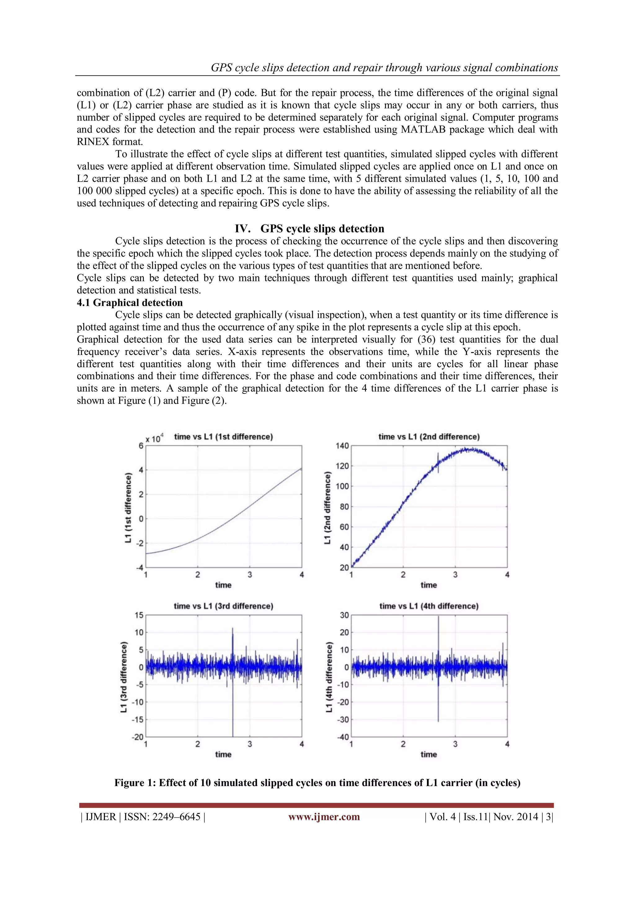
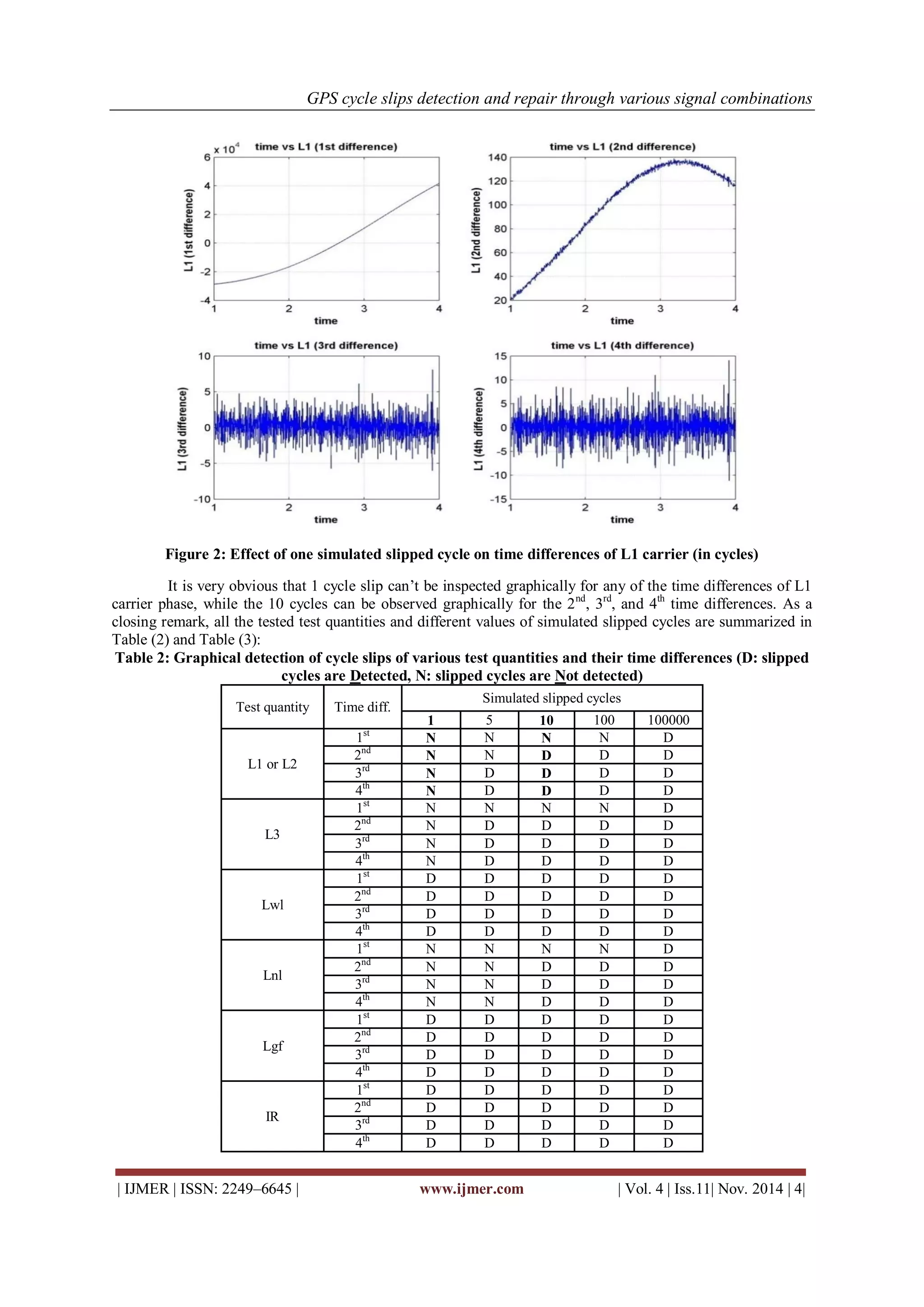
For the detection process, (36) test quantities are used, with variable time differences namely (1st, 2nd, 3rdand 4th time differences) in terms of: (L1) and (L2) carrier phases, (L3) ionospheric free linear combination, (Lwl) wide lane linear combination, (Lnl) narrow lane linear combination, (Lgf) geometric free linear combination, (IR) Ionospheric Residual combination, combination of (L1) carrier and (C/A) code, and

3. GPS cycle slips detection and repair through various signal combinations
| IJMER | ISSN: 2249–6645 | www.ijmer.com | Vol. 4 | Iss.11| Nov. 2014 | 3|
combination of (L2) carrier and (P) code. But for the repair process, the time differences of the original signal (L1) or (L2) carrier phase are studied as it is known that cycle slips may occur in any or both carriers, thus number of slipped cycles are required to be determined separately for each original signal. Computer programs and codes for the detection and the repair process were established using MATLAB package which deal with RINEX format. To illustrate the effect of cycle slips at different test quantities, simulated slipped cycles with different values were applied at different observation time. Simulated slipped cycles are applied once on L1 and once on L2 carrier phase and on both L1 and L2 at the same time, with 5 different simulated values (1, 5, 10, 100 and 100 000 slipped cycles) at a specific epoch. This is done to have the ability of assessing the reliability of all the used techniques of detecting and repairing GPS cycle slips.
IV. GPS cycle slips detection
Cycle slips detection is the process of checking the occurrence of the cycle slips and then discovering the specific epoch which the slipped cycles took place. The detection process depends mainly on the studying of the effect of the slipped cycles on the various types of test quantities that are mentioned before. Cycle slips can be detected by two main techniques through different test quantities used mainly; graphical detection and statistical tests. 4.1 Graphical detection Cycle slips can be detected graphically (visual inspection), when a test quantity or its time difference is plotted against time and thus the occurrence of any spike in the plot represents a cycle slip at this epoch. Graphical detection for the used data series can be interpreted visually for (36) test quantities for the dual frequency receiver’s data series. X-axis represents the observations time, while the Y-axis represents the different test quantities along with their time differences and their units are cycles for all linear phase combinations and their time differences. For the phase and code combinations and their time differences, their units are in meters. A sample of the graphical detection for the 4 time differences of the L1 carrier phase is shown at Figure (1) and Figure (2).
Figure 1: Effect of 10 simulated slipped cycles on time differences of L1 carrier (in cycles)

4. GPS cycle slips detection and repair through various signal combinations
| IJMER | ISSN: 2249–6645 | www.ijmer.com | Vol. 4 | Iss.11| Nov. 2014 | 4|
Figure 2: Effect of one simulated slipped cycle on time differences of L1 carrier (in cycles)
It is very obvious that 1 cycle slip can’t be inspected graphically for any of the time differences of L1 carrier phase, while the 10 cycles can be observed graphically for the 2nd, 3rd, and 4th time differences. As a closing remark, all the tested test quantities and different values of simulated slipped cycles are summarized in Table (2) and Table (3):
Table 2: Graphical detection of cycle slips of various test quantities and their time differences (D: slipped cycles are Detected, N: slipped cycles are Not detected)
Test quantity
Time diff.
Simulated slipped cycles
1
5
10
100
100000
L1 or L2
1st
N
N
N
N
D
2nd
N
N
D
D
D
3rd
N
D
D
D
D
4th
N
D
D
D
D
L3
1st
N
N
N
N
D
2nd
N
D
D
D
D
3rd
N
D
D
D
D
4th
N
D
D
D
D
Lwl
1st
D
D
D
D
D
2nd
D
D
D
D
D
3rd
D
D
D
D
D
4th
D
D
D
D
D
Lnl
1st
N
N
N
N
D
2nd
N
N
D
D
D
3rd
N
N
D
D
D
4th
N
N
D
D
D
Lgf
1st
D
D
D
D
D
2nd
D
D
D
D
D
3rd
D
D
D
D
D
4th
D
D
D
D
D
IR
1st
D
D
D
D
D
2nd
D
D
D
D
D
3rd
D
D
D
D
D
4th
D
D
D
D
D

5. GPS cycle slips detection and repair through various signal combinations
| IJMER | ISSN: 2249–6645 | www.ijmer.com | Vol. 4 | Iss.11| Nov. 2014 | 5|
Table 3: Graphical detection of cycle slips of various test quantities and their time differences (D: slipped cycles are Detected, N: slipped cycles are Not detected)
Test quantity
Time diff.
Simulated slipped cycles
1
5
10
100
100000
L1 & C/A
1st
N
N
D
D
D
2nd
N
N
D
D
D
3rd
N
N
D
D
D
4th
N
N
D
D
D
L2 & P
1st
N
N
D
D
D
2nd
N
N
D
D
D
3rd
N
N
D
D
D
4th
N
N
D
D
D
As a closing remark, it is obvious that not all cycle slips can be detected graphically especially that slips which have small values, thus another approach should be followed in detecting cycle slips which are the statistical approach.
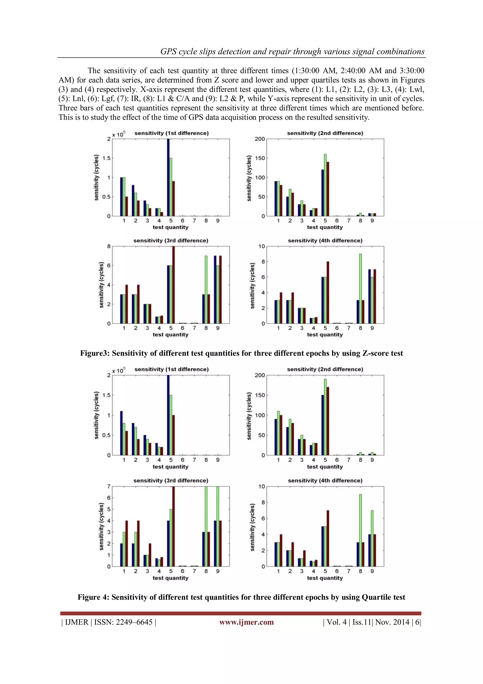
4.2 Statistical tests for outlier (cycle slips) detection Cycle slip could be considered to be an outlier in any data series [10]. Outlier is defined as “an observation (or subset of observations) which appears to be inconsistent with the remainder of that set of data”. However, the identification of outliers in data sets is far from clear given that suspicious observations may arise from low probability values from the same distribution or perfectly valid extreme values for example. There are many methods to reduce the effect of outliers; one of the most used alternatives is the robust statistics which solves the problem of removing and modifying the observations that appear to be suspicious. In some situations robust statistics are not practical, thus it is important to investigate the causes of the possible outliers, and then remove only the data points clearly identified as outliers. There are many statistical tests for outlier detection, here the most two famous ones are used and will be illustrated in the next subsection namely Z-score and lower and upper quartiles 4.2.1 Z-score A Z- scores outlier detector is used to identify any outlier in the data set. Z scores are based on the property of the normal distribution [10] 푍푠푐표푟푒푠= 푥푖−푥 푠 (1) Where 푠= (푥푖−푥 )2푛푖 =1 푛−1 Where푥푖: is a data sample, 푥 : is the mean value, s: is the standard deviation, n: is the number of the data set A common rule considers observations with |Z scores| greater than 3 as outliers. This method has a main disadvantage which is both the mean value and the standard deviation is greatly affected by the outliers [10]. 4.2.2Lower and upper quartile
Lower and upper quartile method is considered a good outlier detector. The main idea of this statistical test is creating lower and upper limits (fences) for the observations, while these fences depend on three main elements. The first element is called the first quartile (Q1) which is the middle number between the smallest number and the median of the data set, while the second quartile (Q2) is the median of the data and the third quartile (Q3) is the middle value between the median and the highest value of the data set, see Equations (2) and (3): 퐿표푤푒푟 푓푒푛푐푒=푄1−1.5∗ 퐼푄푅 (2) 푢푝푝푒푟 푓푒푛푐푒=푄3+1.5∗ 퐼푄푅 (3) Where IQR is called inter-quartile range which is measure of statistical dispersion and is equal to the difference between the third quartile (Q3) and the first quartile (Q1) as shown in equation (4): 퐼푄푅=푄3−푄1 (4) Any data lying outside the defined boundary can be considered an outlier (i.e. any data below the lower fence or above the upper fence can be considered as an outlier).The sensitivity of each test quantity is studied to determine the most suitable and sensitive test quantity for cycle slip detection. Sensitivity is defined as the number of slipped cycles which can be detected at a test quantity by using any statistical tests for outliers’ detection.

6. GPS cycle slips detection and repair through various signal combinations
| IJMER | ISSN: 2249–6645 | www.ijmer.com | Vol. 4 | Iss.11| Nov. 2014 | 6|
The sensitivity of each test quantity at three different times (1:30:00 AM, 2:40:00 AM and 3:30:00 AM) for each data series, are determined from Z score and lower and upper quartiles tests as shown in Figures (3) and (4) respectively. X-axis represent the different test quantities, where (1): L1, (2): L2, (3): L3, (4): Lwl, (5): Lnl, (6): Lgf, (7): IR, (8): L1 & C/A and (9): L2 & P, while Y-axis represent the sensitivity in unit of cycles. Three bars of each test quantities represent the sensitivity at three different times which are mentioned before. This is to study the effect of the time of GPS data acquisition process on the resulted sensitivity.
Figure3: Sensitivity of different test quantities for three different epochs by using Z-score test
Figure 4: Sensitivity of different test quantities for three different epochs by using Quartile test

7. GPS cycle slips detection and repair through various signal combinations
| IJMER | ISSN: 2249–6645 | www.ijmer.com | Vol. 4 | Iss.11| Nov. 2014 | 7|
It is very obvious that the sensitivity improved when the time differences increase for different test quantities, (i.e. the sensitivity of the 4th time difference is much more better than the sensitivity of the 1st time difference for any test quantity except for (L1) & C/A and (L2) & P combinations)
For anytime difference, the Lgf and IR are the most sensitive test quantities as the sensitivity of both reach to less than one cycle, while the sensitivity of (L1) & C/A and (L2) & P combinations ranges between 3 to 8 cycles, while the Lnl considered to be the worst test quantity. It is concluded that the sensitivity differ from time to another for the same data series; as it is function in the error budget of the received signal in different times.
V. Repair of GPS cycle slips
Cycle slip repair process takes place after detecting the time of occurrence of cycle slips at a certain epoch. L1 and L2 carrier phase along with their time differences are used in the repairing process. There are two different methods used here in this research for the purpose of repair cycle slips: Cycle slips repair using average method and time difference geometry. 5.1Cycle slips repair using average method The main idea of the average method for cycle slips repair depends on after detecting the epoch at which the slipped cycles occur, the values of L1 or L2 time differences at this epoch will be removed, and then replace these contaminated values with the average values of the time differences of L1 or L2, then the values of the slipped cycles can be obtained by subtracting the contaminated values from the average values. The average values can be obtained through two main trials:
1. Taking the average values for the 2 epochs just after and just before the contaminated epochs.
2. Taking the average values for all the epochs excluding the contaminated epochs (i.e. the average for all the data except the biased epochs).
5.2 Cycle slips repair using time difference geometry method The main idea of this method depends on the scheme of time difference of the effect of the cycle slips on the L1 or L2 carrier phase time differences as shown in Table (4). It is very obvious from the scheme of time difference, that the 1st time difference is affected by the slipped cycles at an epoch with value of these slipped cycles; while the 2nd time difference is affected by the cycle slips at a zone of 2 successive epochs with the values of these slipped cycles; but for the 3rd time differences, it is contaminated at a zone of 3 epochs and finally the 4th time difference is affected by the slipped cycles at a zone of 4 epochs. The number of slipped cycles can be directly obtained from the 3rd and 4th time differences using all possible combinations of resulted differences Table 4: represents the effect of cycle slips of value Є on the scheme of time differences of carrier phase observations (y: represent various time differences)
Ti
y(ti)
y1
y2
y3
y4
t1
0
0
t2
0
0
0
0
t3
0
0
0
0
0
t4
0
0
Є
0
Є
t5
0
Є
-3Є
Є
-2Є
t6
Є
-Є
3Є
0
Є
t7
Є
0
-Є
0
0
t8
Є
0
0
0
0
t9
Є
0
0
t10
Є
The uncertainty of each time difference for both L1 and L2 carrier phase and its time differences are studied, which is the accuracy of obtaining the integer number of the slipped cycles. In the repairing process, the

8. GPS cycle slips detection and repair through various signal combinations
| IJMER | ISSN: 2249–6645 | www.ijmer.com | Vol. 4 | Iss.11| Nov. 2014 | 8|
uncertainty of each method is studied as shown in Tables (5), (6) and (7). Three columns express the uncertainty of each time difference for all data for each table of different data:
1. The first column expresses the uncertainty in units of cycles, fraction of cycles are used.
2. The second one represents the uncertainty in units of cycles; integer numbers of cycles are used.
3. The third column expresses the uncertainty in units of meters, to show the effect of the slipped cycles on the distance between the receiver and the satellites.
Table 5: Uncertainty using average method of satellite at three different times
Carrier
Time
Time diff
Average between the biased epochs
Average for all data
Cycles
Integer cycles
m
Cycles
Integer cycles
m
L1
1:30:00
1st
0.662
1
0.126
24038
24038
4574.2
2nd
0.609
1
0.116
46.733
47
8.893
3rd
1.434
1
0.273
0.094
0
0.018
4th
3.654
4
0.695
2.517
3
0.479
L2
1st
0.52
1
0.127
18731
18731
4574.2
2nd
0.477
0
0.116
36.411
36
8.892
3rd
1.104
1
0.27
0.066
0
0.016
4th
2.871
3
0.701
1.96
2
0.479
L1
2:40:00
1st
0.028
0
0.005
13462
13462
2561.8
2nd
0.86
1
0.164
1.124
1
0.214
3rd
1.175
1
0.224
1.087
1
0.207
4th
2.204
2
0.419
0.621
1
0.118
L2
1st
0.018
0
0.004
10490
10490
2561.8
2nd
0.67
1
0.164
1.964
2
0.48
3rd
0.926
1
0.226
1.079
1
0.264
4th
1.708
2
0.417
4.018
4
0.981
L1
3:30:00
1st
1.376
1
0.262
254.46
254
48.422
2nd
0.036
0
0.007
3.06
3
0.582
3rd
1.67
2
0.318
0.327
0
0.062
4th
7.94
8
1.511
2.894
3
0.551
L2
1st
1.069
1
0.261
198.15
198
48.389
2nd
0.032
0
0.008
0.385
0
0.094
3rd
1.304
1
0.319
3.3
3
0.806
4th
6.194
6
1.513
4.297
4
1.049
Table 6: Uncertainty of the 7 trials of 3rdtime difference using time diff. geometric method
Trials
L1
L2
Cycles
m
Nearest cycle
Cycles
m
Nearest cycle
(ξ)
0.041
0.008
0
0.039
0.01
0
(-2ξ)
0.662
0.126
1
0.52
0.127
1
(ξ)
0.147
0.028
0
0.126
0.031
0
(ξ,-2ξ)
0.455
0.087
0
0.36
0.088
0
(ξ,ξ)
0.094
0.018
0
0.082
0.02
0
(-2ξ,ξ)
0.491
0.093
0
0.389
0.095
0
(ξ,-2ξ,ξ)
0.378
0.072
0
0.301
0.074
0

9. GPS cycle slips detection and repair through various signal combinations
| IJMER | ISSN: 2249–6645 | www.ijmer.com | Vol. 4 | Iss.11| Nov. 2014 | 9|
Table 7: Uncertainty of the 15 trials of 4thtime difference using time diff. geometric method
Trials
L1
L2
Cycles
m
Nearest cycle
Cycles
m
Nearest cycle
(ξ)
2.519
0.479
3
1.961
0.479
2
(-3ξ)
0.455
0.087
0
0.36
0.088
0
(3ξ)
0.491
0.093
0
0.389
0.095
0
(-ξ)
0.242
0.046
0
0.16
0.039
0
(ξ,-3ξ)
0.288
0.055
0
0.22
0.054
0
(ξ,3ξ)
0.262
0.05
0
0.199
0.048
0
(ξ,-ξ)
1.381
0.263
1
1.061
0.259
1
(-3ξ,3ξ)
0.473
0.09
0
0.374
0.091
0
(-3ξ,-ξ)
0.281
0.053
0
0.23
0.056
0
(3ξ,-ξ)
0.307
0.059
0
0.252
0.061
0
(ξ,-3ξ,3ξ)
0.046
0.009
0
0.041
0.01
0
(ξ,-3ξ,-ξ)
0.279
0.053
0
0.208
0.051
0
(-3ξ,3ξ,-ξ)
0.371
0.071
0
0.298
0.073
0
(ξ,3ξ,-ξ)
0.258
0.049
0
0.191
0.036
0
(ξ,-3ξ,3ξ,-ξ)
0.01
0.002
0
0.016
0.004
0
It is found from the uncertainty of the 1stand 2nd time differences for the average of all data considered to be the worst fixation methods, while the uncertainty of the 4th time difference for both trials range between 2 and 8 cycles which can be considered to be unpleasant fixation method, while the uncertainty of the other trials range between 0 and 3 cycles which is reasonable for the fixation procedure.
Any of these trials can be used in the fixation process (7 trials for the 3rd time difference or 15 trials for the 4th time difference) as they range from 0 to 1 cycle for the majority of all trials.
VI. Conclusion
Based on the used data and the obtained results, many important conclusions are extracted from this paper, these conclusions are going to be categorized according to the detection and repair methods at first, followed by a summary of obtained conclusions:
6.1 Graphical detection
All the test quantities are graphically interpreted when there are very large numbers of slipped cycles (100000 cycles) at a certain epoch.IR and Lgf along with their time differences are considered to be the most sensitive test quantities as they are affected by very small values of cycle slips reach to 1 cycle or less.
6.2 Detection by (Z score) and (Quartiles)
1. 3rd and 4th time differences are more sensitive than 1st and 2nd time differences for test quantities L1, L2, L3, Lwl, Lnl.
2. 2nd time difference is more sensitive than 1st time differences for all test quantities except L1&C/A combinations, L2&P combinations, Lgf, and IR.
3. 3rd and 4th time differences gives almost the same sensitivity for all test quantities, however they may vary in 1 cycle in some test quantities.
4. For test quantities L1&C/A combinations and L2&P combinations: the 1st time difference is more sensitive than 2nd, 3rd and 4th time differences, the same for Lfg and IR
5. L3 for all time differences are more sensitive than L1 and L2 for all time differences.
6. Lwl for all time differences are more sensitive than L1, L2, and L3 for all time differences.
7. Lnl for all time differences are the worst sensitive test quantities.
8. Lgf& IR for all time differences are the most sensitive test quantities.
6.3 Comparing between sensitivity by using (Z score) and (Quartiles)
1. Z score is better than quartiles in sensitivity for both 1stand 2ndtime differences for all test quantities.
2. Quartile is better than Z score for both 3rdand 4thtime differences for all test quantities.
3. Quartile has the advantage; that it can detect both very small and very large slipped cycles at the same data series without needing to make a loop conditions at formulated programs.

10. GPS cycle slips detection and repair through various signal combinations
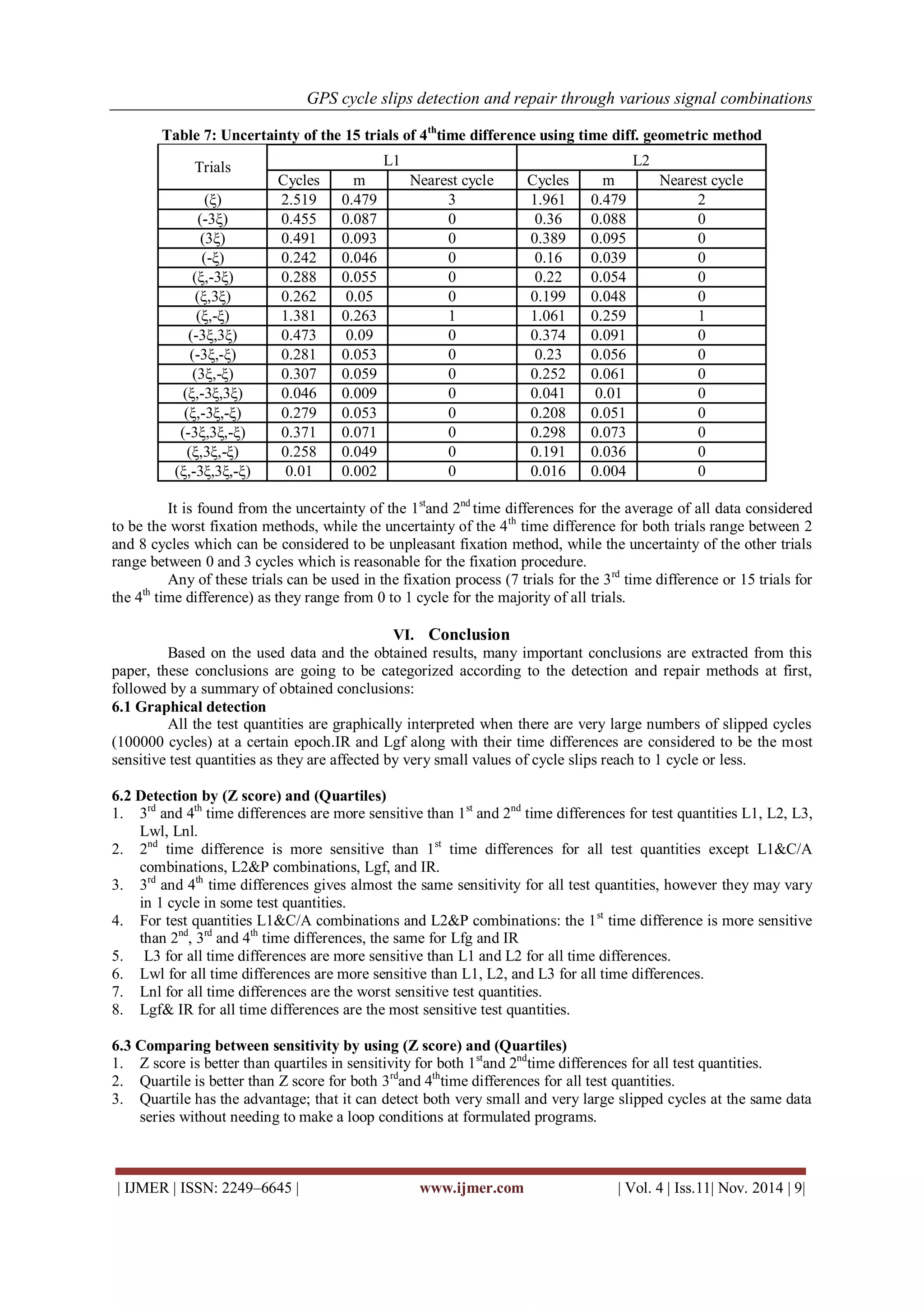
| IJMER | ISSN: 2249–6645 | www.ijmer.com | Vol. 4 | Iss.11| Nov. 2014 | 10|
6.4 Repair by average method
1. For 1st and 2nd time differences: average between biased epochs is better than average for all data
2. For 3rdand 4th time differences: average between biased epochs is less than average for all data
3. 1st time difference average for all data is the worst repair method.
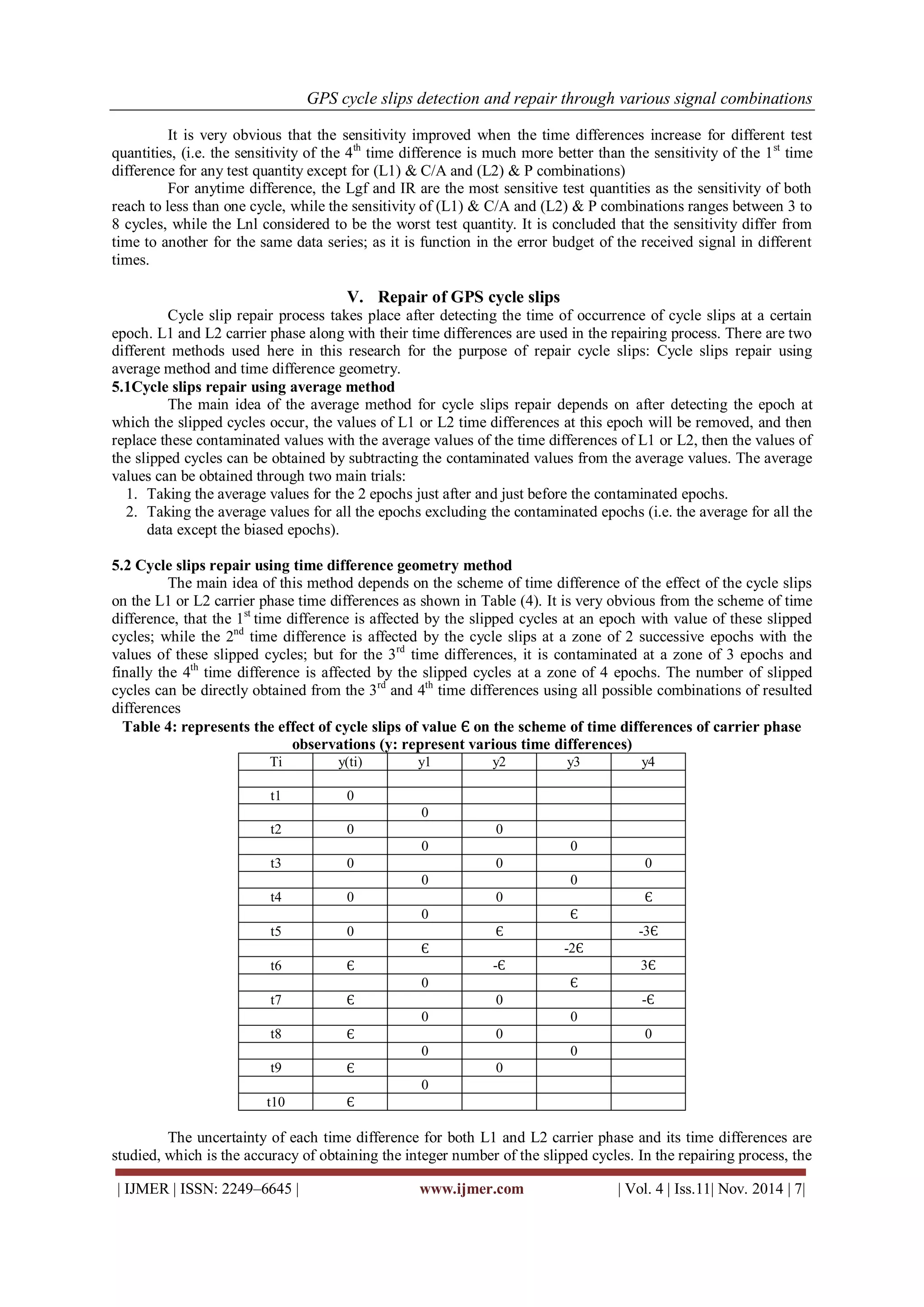
6.5 Repair by geometric method
For all data series, any of these trials can be used (7 trials for the 3rd time difference or 15 trials for the 4th time difference) as it ranges for 1 cycle only for the majority of all trials.
6.6 Overall Summary
Graphical detection method can be considered as a primary stage for cycle slips detection, while the statistical tests (Z-score or quartiles) for cycle slips detection are considered to be more reliable than graphical detection thus they identify the occurrence of the cycle slips at specific epochs. In case of using dual frequency receivers data series any time difference for Lgf or IR can be used as test quantities for the cycle slip detection by any statistical tests, while in case of using single frequency receivers data series, 1st time difference of L1 and C/A combination can be used as test quantity for the cycle slip detection by any statistical tests.
There are many factors affect the sensitivity of the detection procedure which are: the time span of the observations, type of the used receiver (single or dual), the type of used antenna, the type of test quantity, type of the used statistical test, and the existence of large signal noise, ionospheric effect, multipath, and other biases. There are many factors affect the uncertainty of the repair procedure which are: the time span of the observations, and the existence of large signal noise, ionospheric effect, multipath, and other biases. Any trial can be used for the cycle slips repair by geometric method and average method except for the 1st and 2nd time differences for the average for all data as they give very low accuracy of the cycle slip fixation.
REFERENCES
[1] El-Rabbany, A., 2002, “Introduction to Global Positioning System (GPS)”, ArtechHousemobile communication series, Boston, London.
[2] Sorour, T.F., 2004, “Accuacy study of GPS surveying operations involving long baselines”, Ph.D. Thesis, Department of public works department, Faculty of Engineering, Ain Shams University, Cairo, Egypt.
[3] Liu, Z., 2011, “A new automated cycle slip detection and repair method for a single dual-frequency GPS receiver”, Journal of Geodesy, 85(3), 171-183.
[4] Hofmann Wellenhof, B., H. Lichtenegger and J. Collins, 2001, “Global Positioning System- theory and practice 5th edition”, Springer, Verlag, New York, USA.
[5] Sorour, T.F., 2010, “A new approach for cycle slips repairing using GPS single frequency Data”,World Applied Sciences Journal 8(3): 315-325, 2010. ISSN: 1818-4952.
[6] Seeber,G., 2003, “Satellite Geodesy: Foundation, Methods and Applications”, Walter de Gruyter, Berlin, New York.
[7] Zhen, D., 2012, “MATLAB software for GPS cycle slips processing”, GPS Solut.(2012) 16:267-272, Springer, Verlag, New York, USA.
[8] Abdel Mageed, K.M., 2006, “Towards improving the accuracy of GPS single point positioning”, Ph.D. Thesis, Department of public works department, Faculty of Engineering, Ain Shams University, Cairo, Egypt.
[9] Yongin Moon, 2004, “Evaluation of 2-Dimensional Ionosphere Models for National and Regional GPS Networks in Canada”, Msc, department of GeomaticsEngineering, Calgary, Alberta, Canada.
[10] Garcia,FAA, 2012, “Tests to identify outliers in data series”, Pontifical Catholic University of Rio de Janeiro- habcam.whoi.edu.