The document presents an overview of the Soil Moisture and Ocean Salinity (SMOS) mission by ESA, detailing its principles of operation and applications for soil moisture retrieval and salinity mapping. It covers relevant concepts in microwave radiometry, introduces different types of radiometers, and explains the mission's goals, including the collection of global soil moisture and ocean salinity data. Additionally, the document discusses technical aspects such as data processing levels, image reconstruction challenges, and the role of the mission in climate prediction and agriculture.

1. © A. Camps, UPC; 2018 1
Su
ESA SMOS (Soil Moisture and Ocean Salinity) Mission:
Principles of Operation and Land Applications
Prof. A. Camps
CommSensLab, Dept. Teoria del Senyal i Comunicacions
Escola Tècnica Superior d’Enginyeria de Telecomunicacions de Barcelona
Universitat Politècnica de Catalunya‐Barcelona Tech, Spain
E-mail: camps@tsc.upc.edu
www.tsc.upc.edu/prs; www.tsc.upc.edu/nanosatlab

2. © A. Camps, UPC; 2018 2
1. Remote Sensing Lab Activities
2. Introduction:
The Water Cycle
Basic concepts on Microwave Radiometry
Real Aperture Radiometers
Synthetic Aperture Radiometers
Real vs. Synthetic Aperture Radiometers
3. ESA’s SMOS Mission
4. Soil Moisture Retrievals and Land Applications
5. Conclusions
Outline

3. © A. Camps, UPC; 2018 3
http://www.tsc.upc.edu/en/research/commsenslab
1. Remote Sensing Lab Activities (i)

4. © A. Camps, UPC; 2018 4
RADAR/SAR MICROWAVE RADIOMETRY LIDAR
http://www.tsc.upc.edu/rs/
1. Remote Sensing Lab Activities (ii)

5. © A. Camps, UPC; 2018 5
2. Introduction (i): The Water Cycle
• Oceans cover ~70% of the surface of the Earth
• The water cycle controls the heat exchange between
land‐oceans‐atmosphere  climate of the Earth
Thermohaline
circulacion and
salinity maps tracers
evaporation ‐
precipitation
Mean sea surface level and
temperature anomalies
during “El Niño” event (1997)
 RISK FORECAST
(floods and/or droughts)
 fisheries...
Water cycle
controls heat exchange
land‐oceans‐atmosphere
 CLIMATE of the EARTH
Soil moisture
 RISK FORECAST
(floods and/or droughts)
 Crop forecast
 desertification
https://www.washingtonpost.com/news/energy-environment/wp/2018/03/14/the-melting-arctic-is-already-messing-with-a-crucial-part-of-the-
oceans-circulation-scientists-say/?utm_term=.b18f9f5f09ad
“The fast-melting Arctic is already messing with the ocean’s circulation, scientists say”

6. © A. Camps, UPC; 2018 6
108 109 1010 1011 1012 1013 1014 1015
10‐20
10‐15
10‐10
Frequency (Hz)
Brightness (W m‐2Hz‐1sr‐1)
Plank’s law Wien’s Law
Rayleigh‐Jeans’ Law
T=300 K
microwaves
SMOS = radiometer = measures spontaneous thermal radiation
Black body radiation:
In thermodynamic equilibrium :
• Absorbs all incident energy
• Emits all absorbed energy
The “brightness” depends on:
• the physical temperature, and
• the frequency.
2. Introduction (ii): Basic concepts on microwave radiometry

7. © A. Camps, UPC; 2018 7
Geophysical parameters
(soil moisture,salinity, etc.)
Wind speed
over the sea
A radiometer measures the power of the signal collected by an antenna
(Rayleigh‐Jeans’ Law)
TB depends on:
• Physical temperature (T)
• Electrical (,,) and geometrical (roughness) parameters
• Antenna orientation and polarization
• Frequency
Directive
Antenna
Z0
Extended source of
thermal radiation
BLACK BODY: P=k T B
T: Physical temperature
“GRAY” BODY: P=k TB B
TB: Brightness temperature
2. Introduction (iii): Real Aperture Radiometers

8. © A. Camps, UPC; 2018 8
CONICAL SCAN PUSHBROOM
• Image formation by scanning the antenna beam towards the pixel.
• Spatial resolution determined by antenna size
• “High” resolution radiometers (x~10 Km) at low frequencies (L‐band)
require very large scanning antennas ( ~20 m)
Real Aperture Radiometers
2. Introduction (iv): Real Aperture Radiometers

9. © A. Camps, UPC; 2018 9
VLA
(radioastronomy)
1 D ESTAR
(‘80s)
2 D MIRAS
(’90s)
              
*
1 2
1
, E b b ,
2
APV u v t t TF
Synthetic Aperture Radiometers
(Socorro, New Mexico)
Image formation without mechanical scan of the antenna.
2. Introduction (v): Synthetic Aperture Radiometers

10. © A. Camps, UPC; 2018 10
         
 
 


   
21
2 2
1 2
T , T
( , )
1
*
B phnnF , ,F
T
Director
cosines
0( , ) ( , )u v x y   
     *
1 2
1 2 1 2
1 1
2B
V u,v = t b tb
k B B G G
Boltzmann’s
constant
Receivers’
Noise Bandwidths
Available Power
Gains
Complex
Cross‐correlation
Spatial
coordinates
Interferometric radiometer observables
= cross‐correlation products among all pairs of signals collected by elements
in the array (“visibility samples”)
( , ) ( , )V u v T     FIdeal case: 2D Fourier transform
(u,v): depend on the antenna spacing and the array geometry
= spatial frequencies where V(u,v) is sampled
Antenna voltage
radiation patterns
Antennas
solid angle    sinsin,cossin, 
Receivers
physical
temperature
Brightness
temperature
Obliquity
factor (cos())
Antenna 1
Antenna 2
x
y
H1(f)
H2(f)
b1(t)
b2(t)
*
1 2b b
complex
correlator
2. Introduction (vi): Synthetic Aperture Radiometers

11. © A. Camps, UPC; 2018 11
1) Relative calibration (image shape)
‐ Error model (distortions, artifacts…)
‐ Internal references (Tcorr, Tuncorr,…)
2) Absolute calibration (image accuracy)
‐ External references
‐ Thot/Tcold, tie points, vicarious calibration
x
y
z

Image is formed at a time in 1 snap‐shot
Synthetic aperture:
2 step calibration
x
y
z
Image is formed pixel by pixel

Real aperture:
1 step calibration
1) Absolute calibration
External references:
Thot, Tcold
2. Introduction (vii): Real vs. Synthetic Aperture Radiometers

12. © A. Camps, UPC; 2018 12
Introduction:
• SMOS is the second Earth Explorer Opportunity Mission of ESA’s
“Living Planet Programme” (selected in May 1999,
among 27 firm proposals)
• Launch date: November 2nd, 2009
• SMOS
Platform = PROTEUS (CNES, France)
Pay Load Module (PLM)= developped by ESA
. EADS‐CASA (Spain) prime contractor
(now “Airbus Defence and Military”)
. Based on MIRAS studies in the 90’s
. First ever 2D synthetic aperture radiometer
for Earth Observation
SMOS PLM
MASS: 330 Kg
POWER: 300 W
PROTEUS
3. ESA’s SMOS Mission (i)

13. © A. Camps, UPC; 2018 13
SMOS is a challenge:
1) New instrument type:
‐ Revision of basic equation
‐ Detailed error modeling  Error correction algorithms
‐ Image reconstruction algorithms
2) New type of Observables:
‐ Multilook & multiangular observations:
‐ Different pixel’s size and orientation
. Noise and accuracy different for each pixel
‐ Polarization mixing:
. Antenna to Earth reference frame transformation
3) L‐band Land and Sea Emission Models:
‐ Wide range of incidence angles (0‐60)
4) Developmnet of new OS & SM algorithms
3. ESA’s SMOS Mission (ii)

14. © A. Camps, UPC; 2018 14
Global and periodic measurement of:
Soil Moisture and Ocean Salinity
Objectives:
3. ESA’s SMOS Mission (iii)
Variable Accuracy Revisit
time
Spatial
resolution
OCEAN Global SSS maps 0.1 psu 10-30 days 200 km
LAND Global SM maps 0.035 m3/m3 3 days 60 km
Vegetation water content 0.2 kg/m2 3 days 60 km
CRYOSPHERE exploratory ? ? ?

15. © A. Camps, UPC; 2018 15
Payload Module configuration & Ground Segment
Payload module (PLM):
‐ Hub with 18 LICEF
(LIght and Cost‐Effective Front‐ends)
‐ 3 arms with 3 segments/arm x 6 LICEFs/segment
‐ Deployment and hold‐on mechanisms
‐ Optical transmission of digitized data from LICEFs
to digital correlator unit in the hub.
Ground Segment:
‐ Scientific data transmission:
X‐band link  ESAC (Spain))
+ Payload Module Data Center (PMDC):
L1/L2 Scientific data processing, archiving,
PLM programming and management with science.
‐ Telemetry data transmission:
S‐band link  Proteus Ground Segment (Satellite control), Toulouse, France
‐ Operation modes: imaging mode (dual polarization & full‐polarimetric)
calibration mode (noise injection, sky pointing, Moon pointing)
3. ESA’s SMOS Mission (iv)

16. © A. Camps, UPC; 2018 16
Height = 755.5 km  0.5 km
Eccentricity=0.001165
Inclination = 98.416470773546
Mean argument of perigee = 90
Mean local time ascending node = 6 h
Mean anomaly = ‐90
Steering angle = 30
Tilt angle = 32  1
Element spacing = 0.875 
Mission Analysis:
3. ESA’s SMOS Mission (v)

17. © A. Camps, UPC; 2018 17
Raw data Data in their original packets, as received from the satellite.
Level 0 Observation data (correlations, NIR), satellite housekeeping data, instrument/payload
housekeeping data.
Level 1a Calibrated visibilities (correlations), consolidated in pole‐to‐pole time‐based segments,
(location of the spacecraft rather than location of the observation data).
Level 1b Snap‐shot maps of radiometrically corrected and calibrated brightness temperature in the
antenna reference frame (Txx, Tyy, and in the full‐polarimetric mode Txy as well), obtained
from the image reconstruction algorithm. Two products are generated at this level with
different visibility function windows over land and over sea.
Level 1c Swath‐based geo‐referenced maps of brightness temperature in the pixel reference frame
(Thh and Tvv, and I=Tvv+Thh) for a number of incidence angles, with auxiliary information:
geographical coordinates and altitude, geometrical pixel properties, sun illumination etc.
Faraday rotation is corrected at this level.
Level 2 Retrieval of SM over land and OS over sea at the same resolution and location as Level 1
source data.
Apply land‐sea mask to locate mixed pixels. Apply appropriate corrections for SM retrieval.
Level 3 Spatial and temporal aggregation of Level 2 data.
SMOS Ground Segment Processing Levels
3. ESA’s SMOS Mission (vi)

18. © A. Camps, UPC; 2018 18
Antenna Positions Spatial frequencies (u,v) Periodic extension
   2
2 2
,
( , )
1
B ph recn
T TF ,
T
  
 
 


  
( , ) ( , )V u v T     F
u
v
x [wavelengths]
y[wavelengths]
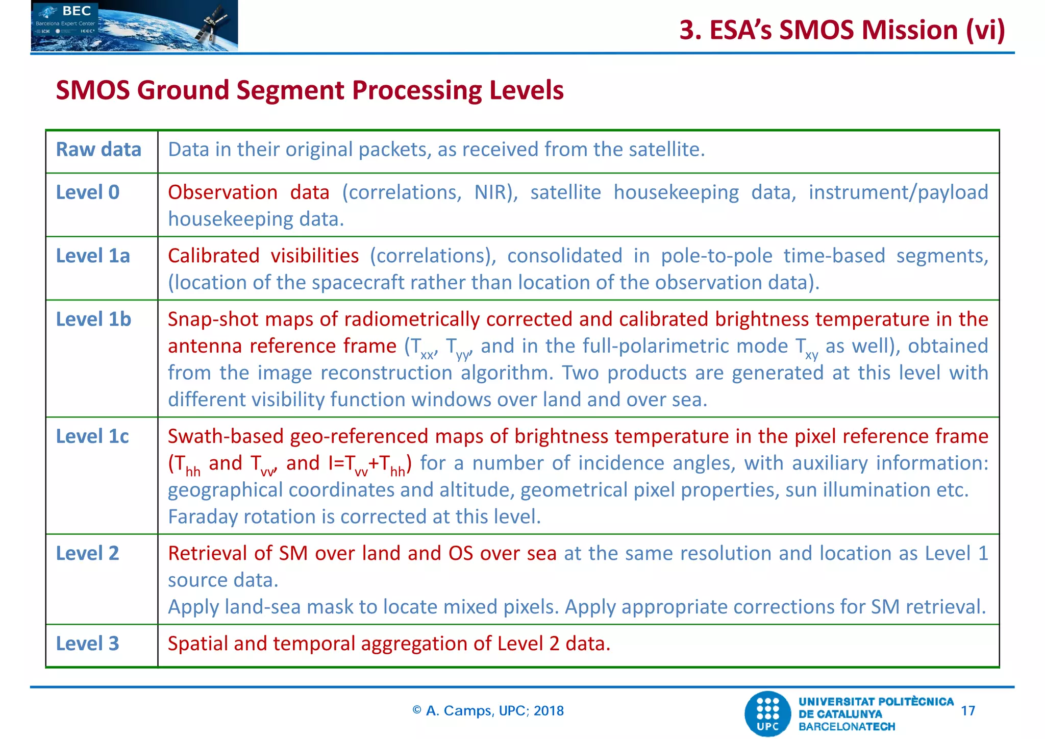
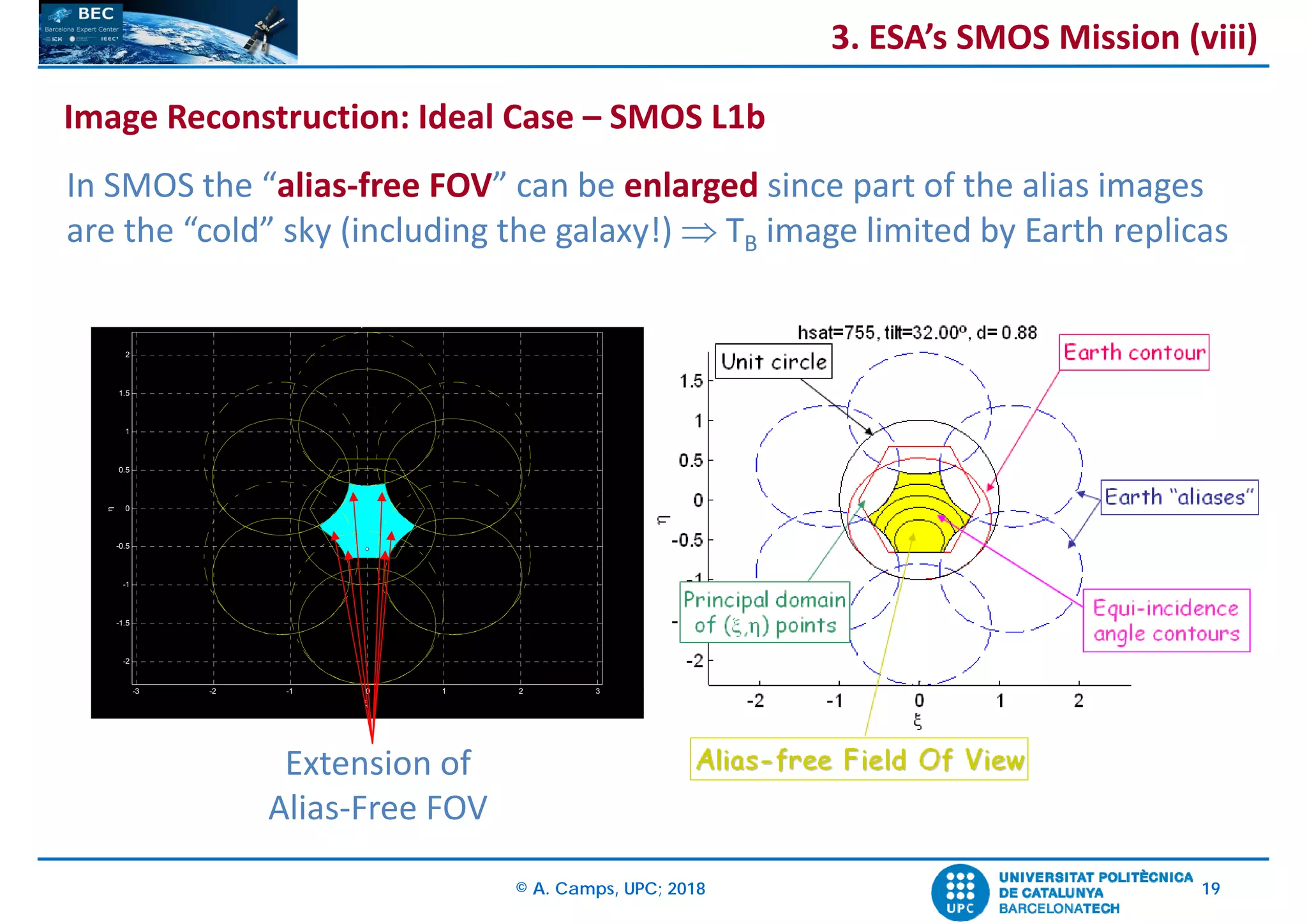
Image Reconstruction: Ideal Case – SMOS L1b
3. ESA’s SMOS Mission (vii)

19. © A. Camps, UPC; 2018 19
In SMOS the “alias‐free FOV” can be enlarged since part of the alias images
are the “cold” sky (including the galaxy!)  TB image limited by Earth replicas
0.8
1 -3 -2 -1 0 1 2 3
-2
-1.5
-1
-0.5
0
0.5
1
1.5
2



Extension of
Alias‐Free FOV
3. ESA’s SMOS Mission (viii)
Image Reconstruction: Ideal Case – SMOS L1b

20. © A. Camps, UPC; 2018 20
SMOS snapshot showing a very strong RFI emission. Note the high
sidelobe levels of RFI emission contaminating the whole image
3. ESA’s SMOS Mission (ix)
Image Reconstruction: The RFI problem (i)

21. © A. Camps, UPC; 2018 21
21
Reconstructed BT using different methods
3. ESA’s SMOS Mission (x)
Image Reconstruction: The RFI problem (ii)

22. © A. Camps, UPC; 2018 22
Geolocalized BT maps and RFI location multi‐look estimation
3. ESA’s SMOS Mission (xi)
Image Reconstruction: The RFI problem (iii)

23. © A. Camps, UPC; 2018 23
Brightness temperatures in the fundamental hexagon of a snapshot over the Atlantic Ocean
strongly affected by an RFI (Radio Frequency Interference) produced by a ship, Y-
polarization. Left, nominal TB; right, nodal sampling TB (Brightness Temperature). A clear
reduction of the general ripples and the sidelobes along the RFI directions can be
appreciated using the nodal sampling technique.
[http://scientiamarina.revistas.csic.es/index.php/scientiamarina/article/view/1667/2162]
RFI mitigation by “nodal sampling”
3. ESA’s SMOS Mission (xii)
Image Reconstruction: The RFI problem (iv)

24. © A. Camps, UPC; 2018 24
• FENIX = RFI canceller: placed between the antenna and the front‐end and
subtracts (most of) the RFI: e.g. GNSS receivers do not loose tracks
“System and Method for detecting and Eliminating
Radio Frequency Interferences in Real Time”
(US Patent No.: 15/222036)
MITIC Solutions SL (UPC spin off)
Hardware‐based RFI detection & mitigation in EO and Navigation
3. ESA’s SMOS Mission (xiii)

25. © A. Camps, UPC; 2018 25
Data processing block diagram in aperture synthesis radiometers
Overpass salinity map
Overpass soil moisture map
Multi‐angular
Emission models
Ancillary data
Snapshot 1
Snapshot 2
Snapshot 3
Snapshot N
Temporal and spatial
averaging
L2 processor
Geophysical parameters retrieval: SMOS L2
3. ESA’s SMOS Mission (xiv)

26. © A. Camps, UPC; 2018 26
No veget.
flat soil
SM=0
No veget.
flat soil
SM=0.4
Dense veget.
Rough soil
SM=0
Dense veget.
Rough soil
SM=0.4
Simulated Tv and Th for different ground- tracks:
Over land: TB depends on: soil moisture, roughness, soil type,
vegetation opacity, albedo and temperaturr
Geophysical parameters retrieval: SMOS L2
3. ESA’s SMOS Mission (xv)

27. © A. Camps, UPC; 2018 27
‐ Availability of global salinity maps, as well as in closed seas and in
cold waters  tracer of marine species  importance for fisheries
‐ As important as soil moisture for agriculture!!
4. Ocean Salinity Retrievals (i)

28. © A. Camps, UPC; 2018 28
BEC ocean products: SMOS advanced global
Ocean salinity: SMOS Debiased non-Bayesian SSS
Advanced L3: 6 years of 9-day, 0.25º OA maps
Advanced L4: 6 years of daily, 0.05º fused maps
Singularity exponents:
Daily maps of SE derived from OSTIA SST,0.25º
4. Ocean Salinity Retrievals (ii)
Singularity exponent (Turiel et al. 2008) is a dimensionless variable that
characterizes the sharpness or regularity of the spatial variation of a
scalar around each point.
Singularity exponents from different variables can directly be compared,
and can be directly associated with the streamlines of the flow

29. © A. Camps, UPC; 2018 29
BEC Ocean products: SMOS Advanced Regional
Improved North Atlantic Ocean and
Mediterranean Sea products
• Debiased non-Bayesian mitigates the
systematic biases (and improves the
coverage.
• DINEOF decomposition allows
characterization and removal of independent
biases
• Multifractal fusion improves the description
of the mesoscale structures
4. Ocean Salinity Retrievals (iii)
Advanced MED L3: 6 years of 9-day, 0.25º OA maps
Advanced MED L4: 6 years of daily, 0.05º fused maps

30. © A. Camps, UPC; 2018 30
BEC Ocean products: SMOS Advanced Regional
Advanced Arctic: 3 years of Arctic, 25-km, 9-day OA maps
(will be extended soon to 8 years)
Best Arctic SSS product (Garcia-Eidell et al, 2017)
4. Ocean Salinity Retrievals (iv)

31. © A. Camps, UPC; 2018 31
‐ Ice thickness maps
5. Ice Thickness Retrieval (i)
https://icdc.cen.uni-
hamburg.de/1/daten/cryosph
ere/l3c-smos-sit.html

32. © A. Camps, UPC; 2018 32
• Global SMOS L3 soil moisture maps (25 km) in near real-time
from 2010 to present at daily, 3-day, 9-day, monthly & annual
time scales
Data access through BEC http://bec.icm.csic.es/
6. Soil Moisture Retrievals and Land Applications (i)

33. © A. Camps, UPC; 2018 33
 global soil
moisture maps
SMOS data is received in real time (<2h) & BEC produces:
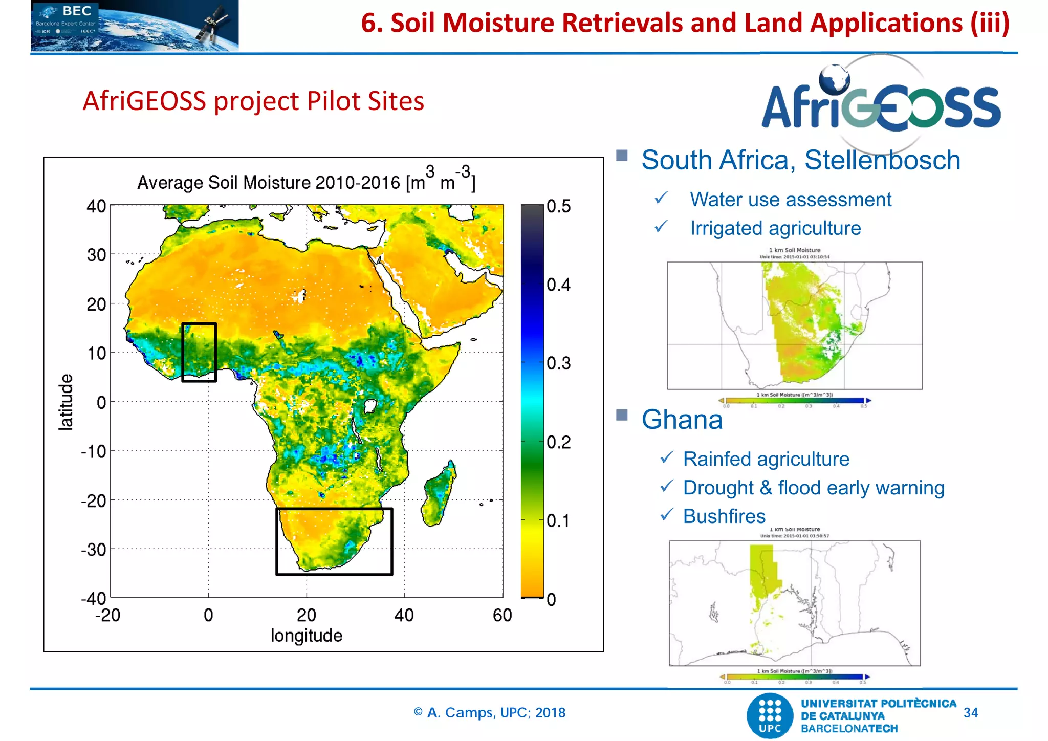
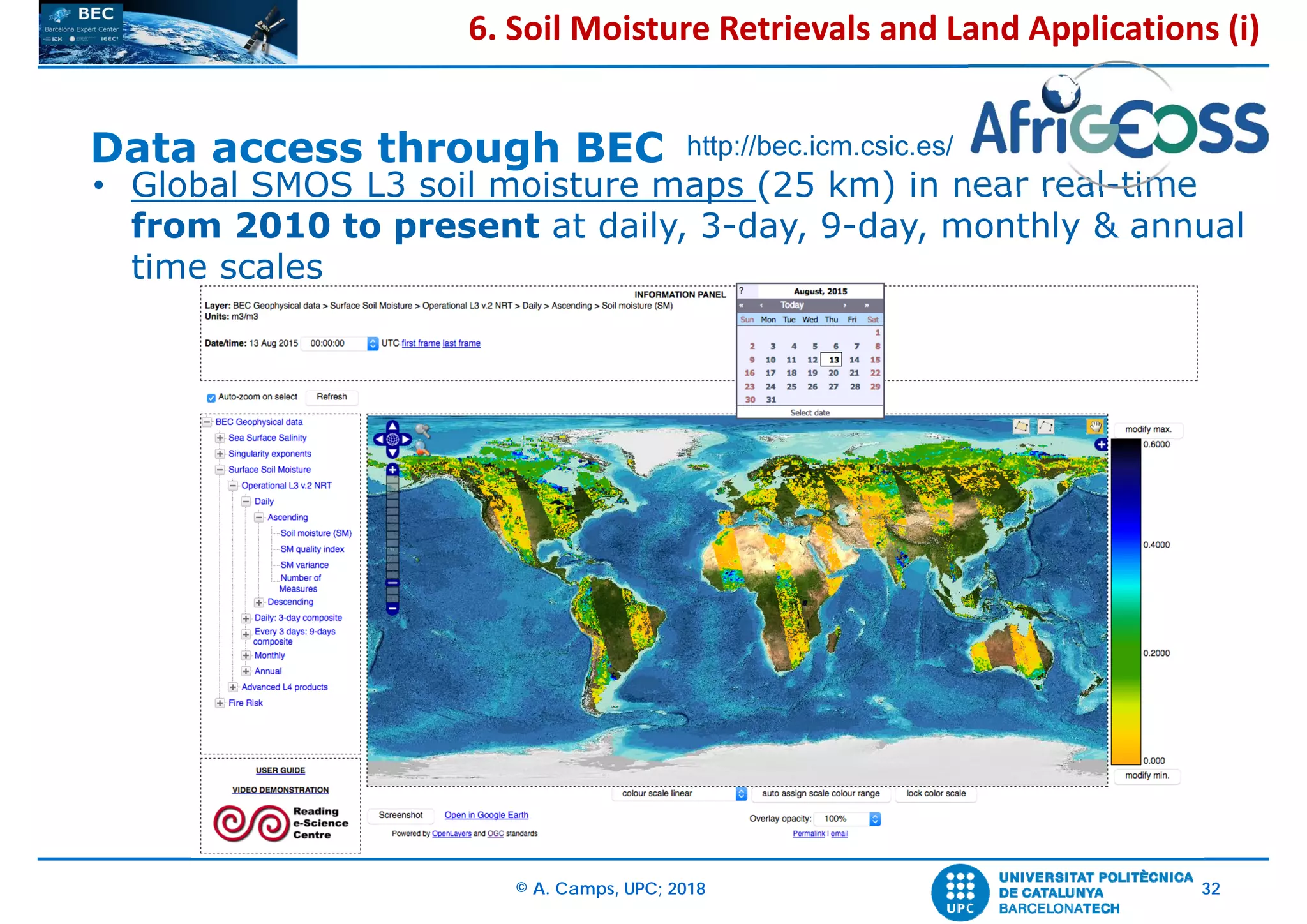
• Global SMOS soil moisture maps (25 km)
• High resolution SMOS/MODIS soil moisture maps (1 km) over 3 pilot sites: IP,
Ghana, South Africa [Piles et al., JSTARS 2015]
high resolution soil
moisture maps 
Data access through BEC http://bec.icm.csic.es/
6. Soil Moisture Retrievals and Land Applications (ii)

34. © A. Camps, UPC; 2018 34
AfriGEOSS project Pilot Sites
6. Soil Moisture Retrievals and Land Applications (iii)
 South Africa, Stellenbosch
 Water use assessment
 Irrigated agriculture
 Ghana
 Rainfed agriculture
 Drought & flood early warning
 Bushfires

35. © A. Camps, UPC; 2018 35
During years 2010-2015 the equatorial Pacific Ocean has been mostly
in a cold phase (La Niña) with the development of the 2015 event
(Godzilla Niño)
Analysis of time series:
Impact of El Niño 2015 event
Difference in SMOS SM (m3/m3) between 2015 and 2013 (Oct-Nov-Dec)
6. Soil Moisture Retrievals and Land Applications (iv)

36. © A. Camps, UPC; 2018 36
6. Soil Moisture Retrievals and Land Applications (v)
Crop yield standardized between 0 (i.e. minimum yield)
and 1 (i.e. maximum yield). Black lines show the states
borders in the study area, which includes North Dakota
(ND), South Dakota (SD), Nebraska (NE), Minnesota
(MN), Iowa (IA), Illinois (IL), Indiana (IN), and Ohio (OH).
The purple box shows the region of Iowa studied.
Scatterplots and regressions for the
relationships between maximum VOD and
crop yield. Yield is standardized between 0
(i.e. minimum yield) and 1 (i.e. maximum
yield). Red‐dashed lines show 95% confidence
intervals.
Relationship between Vegetation Optical Depth and Crop Yield
(using SMAP data)

37. © A. Camps, UPC; 2018 37
 5 categories
 Risk maps produced distributed to regional authorities
Risk categories
Predicted Area (ha) <10 10‐100 100‐1000 1000‐10000 >10000
Risk category Low Moderate High Very high Extreme
Data access through BEC:
Fire Risk Maps over Iberian Peninsula: SM & SST only http://bec.icm.csic.es/
6. Soil Moisture Retrievals and Land Applications (vi)

38. © A. Camps, UPC; 2018 38
OTHER APPPLICATIONS using SM 1km resolution maps
Modelling forest decline occurrence in Catalonia (Spain):
Floods monitoring (Vall d’Aran, North of Spain):
D. Chaparro et al. 2017, JSTARS
6. Soil Moisture Retrievals and Land Applications (vii)

39. © A. Camps, UPC; 2018 39
Soil Moisture influence in Desert Locust development
• Study done in Mauritania by Valladolid University in Spain using Soil
Moisture Maps provided by BEC
• Similar studies ongoing for other insect plagues (Denge in Brazil…)
6. Soil Moisture Retrievals and Land Applications (viii)

40. © A. Camps, UPC; 2018 40
Recent improvements allows to compute high resolution soil
moisture maps at continental scale
e.g. Europe or Australia (possible extension to other parts of the world)
6. Soil Moisture Retrievals and Land Applications (ix)

41. © A. Camps, UPC; 2018 41
Cryosphere: Sea ice concentration & thickness:
Initial phase of production.
3-day, 25 km, polar projection
Land & ocean: Brightness temperature L3:
Development.
1 to 3-day, 0.25º, nodal sampled
Ocean: Sea surface density, global:
Under validation.
Same resolutions as SSS products
BEC Ocean products: forthcoming
7. SMOS BEC Future Products (i)

42. © A. Camps, UPC; 2018 42
Ocean: Sea surface salinity, regional:
Fused SMOS-SMAP 9-km product
BEC Ocean products: forthcoming
7. SMOS BEC Future Products (ii)

43. © A. Camps, UPC; 2018 43
Data, documentation and news @
http://bec.icm.csic.es
7. SMOS BEC Future Products (iii)

44. © A. Camps, UPC; 2018 44
• Basic Microwave Radiometry concepts revised
• SMOS principles presented, with emphasis in imaging and the multi‐
look capabilities
• Concept of geophysical parameters retrieval presented, for oceans
(salinity maps over closed seas and in cold oceans, sea ice
thickness…), and in Soil Moisture (and Vegetation Water content –
Vegetation Optical Depth)
• A number of applications have been presented: for agriculture, crop
yield, forest fires risk, desertification studies and vegetation decline,
flood risk, insect plagues risk…
8. Conclusions (i)

45. © A. Camps, UPC; 2018 45
45
8. Conclusions (ii)
• These techniques can be applied usign airborne
platforms, achieving metric resolution !!
ARIEL radiometer on ICGC (CAT, SP) aircraf

46. © A. Camps, UPC; 2018 46
8. Conclusions (iii)
• … and can be combined with other sensors (e.g. GNSS‐R) to achieve
even better resolution over selected tracks
Sea
Land

47. © A. Camps, UPC; 2018 47
Contact persons:
merce@tsc.upc.edu, camps@tsc.upc.edu
Thanks for your attention!!