This document summarizes the calibration of the broadband photometric system for the RCT 1.3-meter Robotic Telescope. It finds that the linear color transformations and extinction corrections are consistent with similar KPNO facilities, with a photometric precision of 10% at 1 sigma. Some instrumental errors were identified that likely contributed to the overall uncertainty, related to engineering and maintenance issues for the new robotic facility. A preliminary verification showed the calibration solution is robust, perhaps to a higher precision than indicated by the initial calibration. The RCT has been executing regular science operations since 2009.

1. See discussions, stats, and author profiles for this publication at: https://www.researchgate.net/publication/259440793
The RCT 1.3-meter Robotic Telescope: Broad-
band Color Transformation and Extinction
Calibration
Article in The Astronomical Journal · December 2013
Impact Factor: 4.02 · DOI: 10.1088/0004-6256/147/3/49 · Source: arXiv
CITATION
1
READS
46
10 authors, including:
Michael Carini
Western Kentucky University
152 PUBLICATIONS 1,851 CITATIONS
SEE PROFILE
R. Gelderman
Western Kentucky University
53 PUBLICATIONS 312 CITATIONS
SEE PROFILE
Edward F. Guinan
Villanova University
746 PUBLICATIONS 5,101 CITATIONS
SEE PROFILE
C. D. Laney
Western Kentucky University
107 PUBLICATIONS 1,775 CITATIONS
SEE PROFILE
Available from: Edward F. Guinan
Retrieved on: 22 April 2016

2. arXiv:1312.6272v1[astro-ph.IM]21Dec2013
Draft version December 24, 2013
Preprint typeset using LATEX style emulateapj v. 5/2/11
THE RCT 1.3-METER ROBOTIC TELESCOPE: BROAD-BAND COLOR TRANSFORMATION AND
EXTINCTION CALIBRATION
L.-G. Strolger1,2
, A. M. Gott1
, M. Carini1
, S. Engle3
, R. Gelderman1
, E. Guinan3
, C. D. Laney1
, C. McGruder1
,
R. R. Treffers4
, and D. K. Walter5
Draft version December 24, 2013
ABSTRACT
The RCT 1.3-meter telescope, formerly known as the Kitt Peak National Observatory (KPNO)
50-inch telescope, has been refurbished as a fully robotic telescope, using an autonomous scheduler
to take full advantage of the observing site without the requirement of a human presence. Here we
detail the current configuration of the RCT, and present as a demonstration of its high-priority science
goals, the broadband UBVRI photometric calibration of the optical facility. In summary, we find the
linear color transformation and extinction corrections to be consistent with similar optical KPNO
facilities, to within a photometric precision of 10% (at 1σ). While there were identified instrumental
errors likely adding to the overall uncertainty, associated with since-resolved issues in engineering and
maintenance of the robotic facility, a preliminary verification of this calibration gave good indication
that the solution is robust, perhaps to a higher precision than this initial calibration implies. The
RCT has been executing regular science operations since 2009, and is largely meeting the science
requirements set in its acquisition and re-design.
Subject headings: Instrumentation: miscellaneous, methods: observational, methods: statistical, tele-
scopes
1. INTRODUCTION
Robotic telescopes provide a fast and efficient means
to carry out various observations, especially for transient
phenomena or for monitoring work, while mitigating sig-
nificant and often prohibitive travel costs associated with
classical observing. To this end, the 1.3-meter telescope
at Kitt Peak has been restored and refurbished to operate
as a fully autonomous optical facility (Gelderman et al.
2004). The Robotically Controlled Telescope (or RCT)
is operated by an automated and efficient scheduler, and
equipped with a suite of broad and narrow-band filters
to enable ‘snapshot’ imaging and monitoring on a range
of time-scales. The telescope supports the broad in-
terests of the investigators and institutions comprising
the RCT Consortium, and has already contributed to
the locating and monitoring of gamma-ray bursts and
supernovae (McGruder et al. 2004b; Gouravajhala et al.
2012; Gott et al. 2012), ephemerides of minor planets
(e.g., Buie et al. 2013), and the monitoring of vari-
able stars and active galaxies (Engle & Guinan 2011;
Lef`evre et al. 2005; Marchenko et al. 2004; Raiteri et al.
2006; Carini et al. 2004). The RCT is also regularly
used in undergraduate research at Consortium institu-
tions, and frequently contributes to science education
and outreach in programs such as the Arizona Astron-
omy Camp (McCarthy 2011).
Precise photometry is the highest priority to essential
all such science cases. Here, we detail a preliminary pho-
tometric calibration of the RCT 1.3-meter, in the John-
son/Bessell UBVRI-bands, from data obtained from 2010
strolger@stsci.edu
1 Western Kentucky University, Bowling Green, KY 42101
2 present address: Space Telescope Science Institute, Balti-
more, MD 21218
3 Villanova University, Villanova, PA 19085
4 Starman Systems, LLC., Alamo, CA 94507
5 South Carolina State University, Orangeburg, SC 29117
March to 2012 January. This work, in effect, serves as the
first science verification for broadband photometry with
the RCT. It is an automated analysis of numerous and
periodic observations of equatorial standard stars taken
throughout the start of science operations. This analysis
was done largely without a priori corrections or rejec-
tions of data due to short-term variations in observing
conditions, as much of this information was not readily
traced (e.g., via a photometric monitor), as is discussed
later in this manuscript. We do, however, attempt to
isolate data of the best photometric quality for this anal-
ysis, and provide a verification of the precision of the de-
rived extinction and color transformations for the facility.
We also detail possible systematic errors and additional
caveats in using these photometric corrections in other
analyses.
In all, the RCT refurbishment project has been a suc-
cess, meeting nearly all of its initial science requirements.
This manuscript details the current configuration of the
facility, and provides an initial broadband photometric
calibration. In this section we give a brief history of
the facility, and the science motivations behind the re-
furbishment. In §2 we provide an overview of the facil-
ity, detailing the hardware and software essential to its
automation. In §3 we detail the broadband UBVRI cal-
ibration program, its results, and caveats. And in §4 we
provide an overall assessment summary of the refurbish-
ment.
1.1. A Brief History of the RCT
The KPNO 50-inch was developed in the early 1960’s
by the Space Sciences Division at Kitt Peak National Ob-
servatory (KPNO) as an engineering research platform
for the development of remote control protocols for future
orbital telescopes. It was to be operated on Kitt Peak re-
motely from Tucson, AZ via commercial telephone lines,
in a concept in-line with today’s robotic telescopes. The

3. 2 Strolger et al.
telescope was installed in its present location in 1965,
and operated as a remote observatory testbed (Maran
1967b), until 1969 when the facility was converted into
a full-time on site visitor facility. The telescope was
then fitted with an aluminum coated ceramic-vitreous
primary mirror cell replacing a nickel-coated cast alu-
minum cell (Maran 1967a) that warped with changes in
ambient temperature. For the next 25 years, the KPNO
50-inch served as an optical and near-infrared facility for
visiting astronomers, as well as a testbed for National
Optical Astronomy Observatory (NOAO) near-infrared
instruments, such as the Infrared Imager (IRIM), the Si-
multaneous Quad Infrared Imaging Device (SQIID), the
Cryogenic Spectrograph (CRSP), and the Cryogenic Op-
tical Bench (COB). However, budget constraints even-
tually forced decommissioning of the 50-inch as part of
KPNO portfolio in 1996. In 2000, the RCT Consor-
tium successfully bid to operate the telescope (dubbed
the Robotically Controlled Telescope), and completed its
full refurbishment as a robotic instrument in 2009. Tests
of the engineering and optical quality continued through
2012, over which time science programs such as this cal-
ibration program also commenced. It is now fully opera-
tional and open for regular use by the RCT Consortium
partners.
1.2. Overview of Science Requirements for the RCT
The refurbishment and automation of the telescope
was driven by a group of researchers, most of whom
from primarily undergraduate institutions, with comple-
mentary science goals that would benefit from an au-
tomated 1-meter direct imaging facility. Broadly, the
envisioned projects required precise photometric moni-
toring (σmag 0.1) of relatively bright targets ( 20
mag), in visits of a few minutes often executed periodi-
cally over long timespans (weeks to years). The details
of each project set different requirements for photometric
precision, often weighed against acquisition constraints
and practical limits on the overall versatility of the auto-
matic scheduling. Here we focus on a few projects which
demonstrate some of these challenges, and thus exemplify
the science requirements for the RCT.
Measuring Transiting Extrasoloar Planets: An im-
portant goal in probing stellar system evolution is to at
least detect large planets about relatively small stars, as
for example Neptune-sized planets about main sequence
F or G stars. Through the transiting method, the change
in apparent brightness, or transit depth (∆m), is at best
dependent on the relative cross sections of each compo-
nent by:
∆m = −2.5 log 1 −
R2
p
R2
⋆
, (1)
where Rp and R⋆ are the radii of the planet and star
respectively. A Neptune-like planet transiting an F-
star would result in a ∆m of, at most, ∼ 0.001 mag.
This objective places strong constraints on photomet-
ric precision for the telescope. Single-exposure esti-
mates based on the RCT exposure time calculator (RCT-
ETC) suggests σmag ≃ 0.001 should be achievable for
bright (roughly V 14 mag) targets in 2 to 3 minute
exposures (McGruder et al. 2004b). The RCT-ETC
(http://rct.wku.edu/kittpeak/etc.html) is based on
the IRAF task ccdtime, and provides approximate ex-
posure times, S/N, and magnitude limits based on opti-
mized estimates of the site and telescope conditions. We
discuss comparisons to real data in §3.2.
Ephemerides of Minor Planets: Refining the
ephemerides of minor objects in the solar system sys-
tem requires precise astrometry, which is often compli-
cated by the non-sidereal motion of the object itself. The
goal is to obtain sufficient signal-to-noise in exposures
short enough to keep star field trailing significantly be-
low the FWHM of the point spread function (PSF). For
many comets and asteroids this limits exposure times to
only a few tens of seconds, which should be sufficient for
σmag ≤ 0.1 on objects as faint as V ∼ 17 mag.
Monitoring Active Nuclei: Blazar variability moni-
toring, particularly on short timescales, can provide im-
portant clues to the nature of the supermassive black
holes which they harbor. Well-sampled light curves of
the variation in optical continuum provide probes the
size of emission regions that, when combined with com-
plementary data from gamma-ray to radio wavelengths,
provide strong constraints for model conditions of these
AGN. These variations, however, are unpredictable and
irregular occurrences, lasting several minutes or several
years, and thus requiring a level of periodic monitoring
which often challenges classical scheduling at ground-
based telescopes. The objective for the RCT is keep to
an observing cadence for some programs, and use other
periodic programs as fillers to keep the overall schedule
efficient. The automated scheduling of the RCT, as dis-
cussed further in §2.2, is efficient enough to wedge small
programs between optimal windows of larger ones, re-
purpose windows of failed observations, and utilize frac-
tions of nights in marginal or sub-optimal conditions
which might otherwise be lost. This, in combination with
options for repeated requests allows a regular monitor-
ing of blazars ad perpetuum, and provides well-sampled
long-term light curves for complementary studies with,
for example, RXTE, VERITAS, and Fermi (Carini et al.
2004).
Light Curves of Supernovae and Gamma-Ray
Bursts: Both gamma-ray bursts and supernovae are now
routinely discovered at a rate several hundred per year,
respectively, now enabling a more comprehensive under-
standing of the nature of these extremely energetic ex-
plosions. There is still much to ascertain on the most
and the least energetic ranges of both supernovae and
gamma-ray burst optical transients, especially at early
times, or within hours of explosion: most critically for
gamma-ray burst of the shortest duration. Doing so
for a sufficiently large sample will likely require coor-
dinated action from rapid-response observatories, ideally
with queues that can be appended to or reconstructed
automatically (within minutes) to catch high priority
events (McGruder et al. 2004b). As discussed further
in §2.2, the RCT scheduler is designed to take rela-
tive priority of observations into account when build-
ing its schedule, which is rebuilt frequently to accom-
modate new targets throughout night. Coordination on
targets of opportunity will eventually come from large
scale “all-sky” surveys, such as PanSTARRS, SNfactory,
and Palomar Transient Factory (and eventually LSST),
which will act as “event brokers” for the community via
VOEvents, GCN, ATEL, CBET, or other electronic an-

4. The RCT 1.3-meter Photometric Calibration 3
nouncements (Williams et al. 2010).
Narrow-Band Imaging of Resolved Nebulae and
Comets: The RCT is equipped with two large filter
wheels, allowing in addition to standard broadband fil-
ters, immediate access to one of two sets of narrow-
band interference filters. The narrow-band filters are
centered on diagnostic nebular emission lines from H+
,
He++
, S+
, N+
, and O++
in one set, and molecular di-
agnostic lines (with complementary continuum) useful
for comets and minor planets in a second set. These
narrow-band filters extend the versatility of the RCT, al-
lowing 2-dimensional, spacially resolved maps of extinc-
tion (Hα/Hβ), electron temperatures and densities, and
ionization maps for nearby nebulae, and extensive cov-
erage of comets pre- and post-perihelion to monitor out-
burst and fragmentation, determine volatile production
rates, and trace the evolution of the comae (Walter et al.
2004).
2. THE CURRENT CONFIGURATION OF THE RCT
The RCT 1.3-meter is the original Boller & Chivens
Schmidt-Cassegrain on a German equatorial mount, with
the aluminum coated CerVit cell fitted in 1969. The facil-
ity retains the original dome, and still uses the same me-
chanical system in the dome drive and telescope drives,
although most motors have been replaced with newer
models. Most modifications are to the control system
to provide a higher-level control and management of the
telescope, enabling its use as a automated facility. In
this section we detail this current design of the RCT. For
convenience, we provide a brief overview of the facility
in Table 1.
The newest aspect of the RCT 1.3-meter is its tele-
scope control system (TCS) and network of automated
monitors developed by Starman Systems, LLC. The TCS
is designed around an open industrial panel, using a 16-
axis Delta Tau Turbo PMAC to control motors and en-
coders, and an ADAM I/O module for additional digital
and analog functions, and PLDs for complex relay logic
problems such as the mirror covering opening sequence
and dome slit control. Most of the low level automation
software is written in C++, developed at U. C. Berkeley
for the Katzman Automatic Imaging Telescope at Lick
Observatory (Richmond et al. 1993). Basic functionality
uses ASCII protocol communicating over Berkeley sock-
ets.
The automated system coordinates with a few network
services to improve its accuracy. Time data is collected
using the Network Time Protocol daemon, and celestial
calculations are made from in-house code and checked
against SOFA routines.6
JPL Horizons (Giorgini et al.
1996) HTTP calls7
are used for ephemerides of solar sys-
tem objects and to derive non-sidereal track rates. The
TPoint package8
is used for all pointing modeling. All
other software is in-house and non-proprietary.
The automated system also coordinates with a few on-
site monitors. Optional guiding is provided by an auto-
mated guider camera, which locates bright stars within a
6 Software Routines from the International Astronomi-
cal Union Standards of Fundamental Astronomy Collection.
(http://www.iausofa.org)
7 http://ssd.jpl.nasa.gov/horizons.cgi
8 http://www.tpsoft.demon.co.uk
2◦
region of the pointing using the Yale Bright Star Cata-
log,9
zeros pointing to within 20′′
of the original pointing,
and relays continuous corrections to the telescope drive
rates. The system also receives real-time, on-site meteo-
rological information from a Vaisala automatic weather
station,10
which relays humidity, wind, and rain infor-
mation to safety protocols in the dome slit controller.
All image metadata are archived in a SQL database
on-site, which also manages observation requests for the
automated scheduler, described below. Raw images are
stored in the Starbase Database, a managed repository
at Western Kentucky University available to partner in-
stitutions.
2.1. Optical Camera and Filters
The RCT camera operates with a 2048×2048 SITe SI-
424A backside-illuminated CCD with 24 µm pixels. The
CCD is housed in an IRLabs dewar,11
which is cooled to
172K via a closed-cycle, PT-14 gas Polycold refrigeration
system from Brooks Automation, Inc.12
The camera sits
at the f/13.5 Cassegrain focus, to produce a plate scale
of 11.′′
89 mm−1
(0.′′
285 pixel−1
), and an unvignetted
9.′
6 × 9.′
6 field of view.
The filter-wheel assembly sits above the dewar window,
housing a pair of 9-slot filter wheels, within each are 8
circular mounts for 4.5-inch diameter filters and one un-
threaded open mount, to provide a total of 16 possible fil-
ter options (and one double-open position) continuously
available. Table 2 provides a complete list of the filters
available, along with effective wavelengths, bandwidths
(or FWHM), and maximal throughputs.
The RCT broadband set consists of Johnson/Bessell
UBVRI filters from Andover Corporation.13
Figure 1
shows the nominal and effective filter throughputs, cor-
rected for the CCD quantum efficiency, nominal at-
mospheric transmission at zenith from a smoothed
MODTRAN5 model (Berk et al. 2006), dewar window trans-
mission, and primary mirror reflectance, as measured in
2009. These are ideal measures, as factors associated
with degradation and frequency of maintenance reduce
the overall system response, as discussed further in § 3.2.
2.2. Scheduled Observations via the Autonomous
Scheduling Algorithm
While the RCT 1.3-meter can be operated on-site or
remotely, its main function is in a full-robotic imaging
mode. The autonomous scheduling algorithm is an es-
sential component of this observatory, and has been de-
signed to manage numerous requests with various ob-
serving constraints. It is built from the INSGEN list gen-
erator and process spawner originally developed for the
Berkeley Automatic Imaging Telescope (Richmond et al.
1993), which makes scheduling decisions through a least-
cost insertion algorithm.
The method of the INSGEN scheduling algorithm (or
scheduler), as fully described in Richmond et al. (1993),
is as follows. Users provide “requests” which detail ob-
servation information such as the target(s), the number
9 http://tdc-www.harvard.edu/catalogs/bsc5.html
10 http://www.vaisala.com
11 http://www.infraredlaboratories.com
12 http://www.brooks.com
13 http://www.andovercorp.com

5. 4 Strolger et al.
TABLE 1
RCT facility Overview
Location Kitt Peak National Observatory, Arizona
31◦57′12′′ N, 111◦34′ W (WGS84)
Elevation 2040 meters above sea level (approx. 800 meters above horizon)
Optics 1.3-meter Schmidt-Cassegrain, f/13.5 secondary
Plate Scale 11′.89 mm−1, 0′′.285 pixel−1, 9′.6 × 9′.6 FOV
CCD SITe 2048 x 2048 CCD, 24 µm pixels
4 available amplifiers, 1 currently in use (120 sec read time)
Gain (amp C) = 2.56 e− DN−1, Read Noise (amp C) = 15.05 e−
Minimum Full Well signal ≈ 150, 000 e−
dark current ≈ 1 × 10−5 e− s−1 pixel−1
Filters 5 broadband, and 21 narrow-band
Two active wheels with 16 total positions continuously available
Modes of Operation Robotic queue scheduled;
Remote or on-site, scripted or standard observing
TABLE 2
RCT Filter Set
Filter Effective λ (˚A) Bandwidth (˚A) Max. Trans. (%) Model #
Broadband:
U . . . . . . . . . . . . . . . . . . . 3573 900 75 ANDV8303
B . . . . . . . . . . . . . . . . . . . 4265 931 66 ANDV8666
V . . . . . . . . . . . . . . . . . . . 5434 751 89 ANDV8667
R . . . . . . . . . . . . . . . . . . . 6487 1016 84 ANDV8668
I . . . . . . . . . . . . . . . . . . . . 8129 1728 96 ANDV8669
Nebular Narrowband: a
HeII. . . . . . . . . . . . . . . . . 4689 33 66 ANDV8163
Green Continuum #1 4807 53 62 ANDV8164
Hβ . . . . . . . . . . . . . . . . . . 4864 35 63 ANDV8165
[OIII] . . . . . . . . . . . . . . . 5009 25 62 ANDV8166
Green Continuum #2 5313 96 70 ANDV8167
[NII] #1. . . . . . . . . . . . . 5760 30 60 ANDV8168
Red Continuum . . . . . 6459 83 63 ANDV8169
Hα Narrow . . . . . . . . . . 6565 14 38 ANDV8281
Hα Wide . . . . . . . . . . . . 6561 25 51 ANDV8282
[NII] #2. . . . . . . . . . . . . 6594 29 42 ANDV8283
[SII] #1 . . . . . . . . . . . . . 6716 13 51 ANDV8284
[SII] #2 . . . . . . . . . . . . . 6729 14 55 ANDV8285
Comet Narrowband:
OH. . . . . . . . . . . . . . . . . . 3090 62 49 Barr Lot 4108
UV Continuum . . . . . . 3448 84 72 Barr Lot 4108
CN . . . . . . . . . . . . . . . . . . 3870 62 80 Barr Lot 1109
C3 . . . . . . . . . . . . . . . . . . 4062 62 69 Barr Lot 4108
Blue Continuum . . . . . 4450 67 76 Barr Lot 4108
C2 . . . . . . . . . . . . . . . . . . 5141 118 82 Barr Lot 4108
Green Continuum #3 5260 56 80 Barr Lot 1009
NH2 Continuum. . . . . 5660 12 67 Barr Lot 1109
NH2 . . . . . . . . . . . . . . . . . 5721 85 80 Barr Lot 4408
a The nebular filter set was re-scanned in the laboratory in 2012 March.
of exposures, the exposure times, and filters, and the
observing constraints such as the range of airmass, min-
imum angle of Sun/Moon avoidance, or specific start or
end times. Users also assign a priority to their requests,
which in principle can be managed by partner fractions.
The scheduler calculates “windows of opportunity” for
each target in each request based on the target’s rise and
set times, the block length of the request, readout and
slew times, sunrise and sunset, and other constraints.
A “best time” is defined within each window, which
is generally centered at the meridian transit unless oth-
erwise constrained. The scheduler sorts the request list
by priority, and reserves blocks at best times according
to priority. As the scheduler proceeds through the pri-
oritized list, it searches outward from a given request’s
best time for free blocks within the target’s window of
opportunity. If no free window can be identified, the
scheduler then attempts to accommodate the block by
pushing higher priority requests away from their optimal
spots without pushing them out of their observable win-
dows or reordering the sorted list. If this cannot be ac-
complished, the request with the lower priority is skipped
until the following scheduling instance, in which it dis-
cards the original list and starts again.
Scheduling instances are implemented periodically
throughout the daytime hours, and each time an obser-
vation has completed. With each instance, the previ-
ous observation is rejected from the list (if applicable),

6. The RCT 1.3-meter Photometric Calibration 5
400 500 600 700 800 900
Wavelength (nm)
0
20
40
60
80
100
%Throughput
U
B
V R
I
Atmosphere
CCD DQE
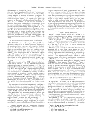
Fig. 1.— The nominal RCT Johnson/Bessell UBVRI filter responses. The dotted lines show the laboratory transmissions for each filter,
and the solid lines show the throughputs after multiplying by the CCD quantum efficiency (at T = 172K) and nominal atmospheric
transmission at zenith (dashed lines). The throughputs are also corrected by measures of the primary mirror reflectance (approximately
87% from 4000 ˚A to 7000 ˚A) and dewar window transmission (approximately 95% from 4000 ˚A to 1µm).
and the allowable windows are re-constrained by either
sunset or the current time, whichever is latest. This al-
lows for real-time ingesting of new observation requests
at any time, even while the telescope is observing, and
significant flexibility to keep a highly efficient schedule,
should a previous request have shorter execution window
than anticipated (usually slew times shorter than the es-
timated 2 minute intervals), or fail due to lack of avail-
able guide stars. Scheduling instances take little time to
execute, usually less than 10 seconds for the hundreds of
active requests currently in the queue.
The INSGEN scheduler operates the RCT with highly
efficient observing plans, over periods of continuous ob-
serving, or without instrument outages or poor weather.
As a measure of the telescope’s efficiency, we show in Fig-
ure 2 the fraction of each night the imager exposed on
fields, which was generally between 40% and 60%. This
efficiency figure includes the CCD readout time for each
exposure, as this is set by the binning mode or similar
details for a specific observation. But the fraction omits
the slew time to each field, filter setup, or guide star ac-
quisition (when applicable) as these are limitations more
inherent to the facility. The remainder of the time was
lost to weather and instrument servicing, with less than
10% spent on field acquisition and other overheads.
The observation requests are collected and logged in
an on-site database, populated by users via a web inter-
face available to partners. There are several convenience
options at the interface, including target resolution via
NED, SIMBAD, JPL Horizons, or via the expanding
RCT database. Users can monitor the schedule via the
same web interface, seeing both tabular and graphical
representations of the scheduled, skipped, and executed
requests.
3. THE PHOTOMETRIC CALIBRATION OF RCT UBVRI
FILTERS
The purpose of this paper is to not only give an intro-
duction to the RCT, but to provide measure of its photo-
metric quality. Observations of Landolt (2009) standard
stars were obtained in several sequences in from 2010
May 25 to 2012 Dec 31. This program took advantage of
the scheduler efficiency to queue periodic observations of
targets at the scheduler’s lowest priority, thereby execut-
ing when the scheduler filled gaps between ideal merid-
ian crossings of higher priority programs. The sequence
executed 3 successive images in each passband, with ex-
posure times of 30 s, 20 s, 10 s, 10 s, and 10 s, in each
U, B, V, R, and I, respectively. The exposures were not
guided to reduce overheads.
The sequence was taken without observing constraint,
allowing for a modest range of airmass and cloud con-
ditions for broad assessment. However, as the goal of
the scheduler is to observe targets as close to meridian
whenever possible, very few observations were actually
executed at large [sec(z) > 1.5] airmass. The supernova
in M101 in 2011 August (SN 2011fe; Nugent et al. 2011)
presented an important target of opportunity, and its low
altitude at KPNO necessitated a set of high airmass stan-
dards for accurate calibration of its observations.14
An
14 The RCT 1.3-meter UBVRI photometry of SN 2011fe is pre-
sented in Gouravajhala et al. (2012) and Gott et al. (2012).

7. 6 Strolger et al.
Nov 2010 May 2011 Nov 2011 May 2012 Nov 2012
UT Date
0.0
0.2
0.4
0.6
0.8
1.0
FractionofNightinSciecneExposures
Fig. 2.— An illustration of the scheduling efficiency of the RCT for a selected date range. The gray impulses indicate the fraction of
each night the telescope exposed on targets, determined from the sum of exposure times and read-out times divided by the length of night
between evening and morning astronomical (18◦) twilights. Field acquisition, time lost to weather, and instrument down times account for
the remainder of these fractions. The black points are binned averages running every 50 nights in which data is taken.

8. The RCT 1.3-meter Photometric Calibration 7
additional standard sequence at airmass > 2.2 was there-
fore added to the request over the observable duration of
SN 2011fe.
As with most observations at the RCT, these standard
star sequences were taken with the CCD binned 2 × 2,
to take advantage of the oversampling of the typical PSF
(approximately 1.′′
5 to 2.′′
5 FHWM) at the site. This re-
sults in a pixel scale of 0.′′
571 ± 0.′′
001 pixel−1
, verified
against catalog solutions in a process described further
in §3.1. Figure 3 indicates which Landolt (2009) stars
were observed and how often. Ultimately, 5, 600+ UB-
VRI sequences of standard stars were taken, of which
approximately 1, 000−2, 000 stars per filter were used in
the final analysis.
3.1. Data Reduction, Photometry, and Calibration
The RCT executes a calibration sequence in a sepa-
rate request, taken nightly or as priority allows. Bias
images were taken in a dark dome (after twilight) as a
precaution, although the instrument shows no evidence
of light leaks and the dark current is estimated to be less
than 1 × 10−5
e−
s−1
. Flat-field correction images were
derived from images of a lamp-illuminated screen on the
interior of the dome, which are done as a matter of course
in at least each of the broadband filters. All science data
in this analysis were bias and dome flat-field corrected
using the IRAF imred.ccdred package, with respective
nightly correction images. Comparisons of a few dome-
flat and bias images yielded a nominal read noise of 15.1
e−
, and gain of 2.6 e−
DN−1
.
Raw RCT images have only an approximate World
Coordinate System map to their pixels. To accu-
rately correlate sources with known positions of stan-
dards, we pattern matched detections (via SExtrator,
Bertin & Arnouts 2010) with the USNO B1 cata-
log (Monet et al. 2003), using a triangle-matching al-
gorithm which solves for linear source-to-source trans-
formations, including shifts, rotations, and changes in
scale, in which the plate scale is a free-parameter. This
automated fitting required greater than approximately
five detections per image, evenly distributed, for accu-
rate matching (to RMS < 0.′′
2). For most observations
in the redder passbands of these standard fields, where
there is greater sensitivity and a larger number of red
sources, this criteria was easily met. But for bluer pass-
bands where there were fewer detected sources, the fail-
ure rate in direct pattern matching was as much as two
times more frequent than for the redder passbands, re-
sulting in about half as many correlated measures.
We may have had more success in pattern matching
if we reduced the free-parameters in the matching algo-
rithm, fixing the plate scale to set value for example,
although it was important to independently verify the
plate scale of the image plane. We might also have made
use of the back-to-back execution of the observing se-
quence to create “detection frames” from combinations
of images, in the same filter or in all-filter combinations.
Although that would have required some slight image-
to-image forced alignment, through cross-correlation or
human source identification, as small (∼ 0.′′
5) drifts be-
tween exposures occur in the sequence when tracking
was momentarily resets. However, the final number of
matched targets were more than sufficient to precisely
determine the photometric transformations, even after
the rejection pass, and so it was not deemed necessary
to put effort into recovering these acceptable losses.
Instrumental aperture photometry was performed in
a 6.5 pixel (3.′′
71) radius on rectified images, scaled by
their exposure times to units of DN s−1
. The aperture
was chosen by determining the growth curve of several
hundred stars in selected images of each passband, as
illustrated in Figure 4, and selecting an aperture consis-
tently near the confusion limit (6 − 7 pixel radii, on av-
erage). This aperture was large enough to accommodate
changes in the PSF due to seeing and other instrumental
effects. Aperture corrections were estimated from ratios
of the encircled energy of a 2-D Gaussian with symmet-
ric FWHM equal to the mean measured FWHM of the
image, at the confusion aperture relative to an infinite
aperture. In all passbands, these corrections were found
to be less than 0.01 mag. However, it is important to
note, as can be seen in Figure 4, that the shape of the
PSF was typically more complex than the 2-D Gaussian
fit. An extreme case due to instrumental failure is also
shown in §3.3.
A first-pass calibrated magnitude (m) was determined
in each filter from the instrumental magnitude using,
m = −2.5 log10(DN s−1
)+Z+A0X+A1(color)+A2X(color),
(2)
where Z is the zero point (magnitude at 1 DN s−1
), A0 is
the airmass term coefficient, A1 is the color term coeffi-
cient (using colors later indexed in Table 3), and A2 is the
airmass × color term coefficient with the same color in-
dices. The calibration coefficients in Equation 2 (Z, A0,
and A1 respectively) were fit via the weighted Levenberg-
Marquardt non-linear least squares algorithm provided
by the IRAF apphot package. The cross extinction-color
corrections (or A2 terms) are often difficult constrain
when simultaneously fit with the color transformations
and first order extinctions, and leaving these terms free
resulted in degeneracies that were inconsistent with the
data. It was expected, however, that these terms would
be negligible, with |A2| < 0.02. We, therefore, fixed at
A2 ≡ 0.0 for all filters throughout this analysis. Fig-
ure 5 shows the difference in instrumental and cataloged
magnitudes as functions of each of the fit parameters.
Equilibrium binned data (11 bins of approximately 250
measures in each bin) and the slopes of the preliminary
photometric calibration coefficients are shown for com-
parison. Note that the fits are to the data, and not to
the binned points.
Figure 6 shows the residuals of the fits, biased to the
initial zero point magnitudes for each filter, with addi-
tional offsets for clarity. The RCT is equipped with a
modest “cloud monitor”, a thermoelectric infrared sky
temperature sensor which compares sky temperature to
ground temperatures to, in principle, derive an approxi-
mate fraction of the sky covered in clouds. The residuals
in Figure 6 are shaded in grayscale by these relative cloud
values. As non-photometric data is inherently fainter,
their measures stream downward on this plot. It is ap-
parent from the figure that the cloud values do little to
discern non-photometric (or otherwise faint) data. At
present, it is unclear if the cloud monitor is too impre-
cise, or inaccurate due to failure, but it would seem that
it is not yet a useful indicator of photometric quality,
and thus insufficient for isolating photometric data for

9. 8 Strolger et al.
0
log(Number of Observations)
0.5 1.0 1.5 2.0 2.5
MARK-A4
MARK-A3
MARK-A2
MARK-A1
MARK-A
F24C
F24B
F24A
F24
F22
F11B
F11A
F11
97-351
95-98
95-97
95-96
95-330
95-302
95-301
95-276
95-275
95-193
95-190
95-16
95-15
95-102
95-101
95-100
92-348
92-342
92-339
0.5 1.0 1.5 2.0 2.5
92-330
92-259
92-253
92-252
92-250
92-249
92-248
92-245
112-822
112-805
111-775
111-773
111-1969
111-1965
111-1925
110-507
110-506
110-504
110-503
110-502
110-499
110-497
110-496
110-450
110-441
110-340
109-71
109-537
109-381
109-231
109-199
108-551
Fig. 3.— Total number of Landolt (2009) standard star observations (gray bars) in the V -band, for each standard indicated on the
ordinate axis. Black bars indicate the number of observations ultimately used in the final analysis.
0 5 10 15 20
Aperture (in arcseconds)
−2.5
−2.0
−1.5
−1.0
−0.5
0.0
0.5
Changeinmagnitudefrompreviousaperture
Growth Curve a100516031.fits.stars
109-231, V-band
Fig. 4.— Example growth curve for stars in one V-band exposure, centered on SA 109-231. Gray points show the change in magnitude
at the set aperture indicated, from the measure in the next smallest aperture, for each of the 167 detections (to 3σ) in the image. Black
points are the mean for all stars in each aperture. The solid line is the expected magnitude change a 2-D Gaussian with an equivalent
FWHM. Dashed lines show the selected confusion aperture (abscissa), and its corresponding aperture correction (ordinate).

10. The RCT 1.3-meter Photometric Calibration 9
-1
0
B
B−V
0
1
2
3
U
U−B
-2
-1
0
minstrumental−mactual
V
B−V
-2
-1
0
R
V−R
1.2 1.6 2.0 2.4
Airmass (A0 )
-2
-1
0
I
0.0 1.0 2.0
Color (A1 )
V−I
0 1 2 3 4 5 6
Airmass ×Color (A2 )
Fig. 5.— Difference in instrumental and cataloged standard star measures, as functions of fit parameters Airmass, Color, and Airmass ×
Color (gray points). The black points are equilibrium binned data, with approximately 250 points in each bin, where the errorbar width
represents the bin width. The lines slopes are the A0 and A1 coefficients for each passband and color indicated. The cross extinction-color
coefficient is fixed to A2 ≡ 0.0.
this analysis.
The distribution of residuals in the fits do, however,
provide a guide for isolating photometric data. The his-
tograms inset to the right of Figure 6 show the distribu-
tion of the residuals relative to the zero points derived in
this first pass analysis. As one would expect, these distri-
butions grossly show modes near the bright end of each
calibrated set, with skewed smaller populations trailing
toward the faint end from gradually less photometric ob-
servations. However, there also appears to be bimodality
in the distributions, with fainter secondary loci located
the tail of the distributions, most visibly in the B-band
set. Such distributions could result from data obtained
in systematically similar (and unfavorable) weather con-
ditions, or from a systematic error in the functionality of
the telescope. We discuss some likely possibilities, with
focus on the latter, in §3.3. For the sake of furthering
this analysis, we assume these two populations are dis-
tinct, and can be reasonably separated into photometric
and non-photometric (or otherwise obscured) sets. We
fit bi-modal Gaussian probability distribution functions
(PDFs) to the histograms, solving for the mean and stan-
dard deviation of each mode. These distributions are
over-plotted on the histograms of Figure 6.
We then performed a second-pass analysis, following
the same apphot procedure to determine calibration co-
efficients outlined at the beginning of this section, on
only the data constrained within 1σ of the bright modes
in the histograms of Figure 6. The results of this final
pass are shown in Figure 7, and and the final calibration
coefficients are shown in Table 3.
3.2. Verification of the Photometric Calibration
The final derived color transformation coefficients are
in excellent agreement with available data from compa-
rable telescopes with optical imagers and similar broad-
band filters at KPNO, specifically the WIYN 0.9-meter
and the KPNO 2.1-meter (Massey et al. 2002). The ex-
tinction coefficients are reasonably similar, although our
analysis has been carried out to larger airmasses than
presented by Massey et al. (2002). As discussed previ-
ously, no attempt was made to fit the airmass × color
terms for possible atmospheric reddening, as it was as-
sumed the effect was negligible. The lack in notable trend
in the data of Figures 5 and 7 generally confirm this as-
sumption.
The photometric calibration coefficients were deter-
mined with total errors in the mean of less than 0.3%.
The photometric errors (or errors in the calibration, pre-
sented as 1σ errors in Table 3) are also very reasonable,
although there may be systematic contributions to these
residuals attributable to faults in the facility: a likeli-
hood further discussed in §3.3. As an independent test,
these photometric corrections were applied to the early
RCT direct imaging data of SN 2011fe, obtained at aver-
age airmass of 1.9. The results shown in Figure 8 are in
excellent agreement with data from various observatories
of this nearby Type Ia supernova.
As another test of the calibration quality, we compared
the calibrated magnitudes of all 22, 059 data points to
their measured photometric errors, in a signal-to-noise
comparison shown in Figure 9. The figure shows an or-
derly agreement between the calibrated magnitudes and

11. 10 Strolger et al.
2011 2012 2013
UT Date
18
20
22
24
26
28
ZeroPointMagnitude(Vega)
U−2
B−2
V
R+2
I+4
0.00 0.17 0.33 0.50 0.67
Fig. 6.— Residuals of the photometric calibration shown at the respective zero point magnitudes for each passband (dashed line). Data
are shown in grayscale illustrating their relative cloud value, indicated by the color bar above the diagram. Insets to the right of the figure
show histograms of calibrated data (shaded), centered at the respective zero point lines. Over-plotted lines show the bi-modal Gaussian
PDFs fit to the histograms. Data is offset by additional values annotated, for clarity.
TABLE 3
UBVRI Extinction and Color Transformation for the RCT 1.3-meter
Filter Zero Point Airmassa Color Terma 1σ Error N meas.
(Z) (A0) [A1(color)]
U . . . 20.316 ± 0.003 -0.924 0.277 (U − B) 0.10 910
B . . . 22.550 ± 0.002 -0.712 -0.005 (B − V ) 0.06 1281
V . . . 22.785 ± 0.002 -0.499 0.005 (B − V ) 0.06 1284
R . . . 23.001 ± 0.002 -0.448 0.016 (V − R) 0.07 1993
I . . . . 22.513 ± 0.001 -0.386 0.012 (V − I) 0.06 2167
a Standard Deviation of the Mean in Airmass and Color terms are all less
than 0.001.
the measured magnitude errors that would otherwise be
absent (resulting in increased scatter along the abscissa)
if the calibration were inaccurate. There are two is-
sues, however, to note. First, the trend in increasing
noise occurs at much shallower magnitudes (by factors
of 2 − 4) than expected from estimates in signal-to-noise
given by the RCT-ETC, given the appropriate exposure
times, seeing conditions, and average sky brightnesses.
Some deviation from these ideal estimates are expected,
as the overall system response changes over time. It is
not likely this is an issue with the aluminization of the
primary, as measures of the reflectivity of the primary
mirror have changed little since 2009, and are appro-
priately accounted for in the RCT-ETC models. The
atmospheric corrections used in the RCT-ETC are also
well matched to the MODTRAN5 models for the site. It is
most likely this is a degradation in the broadband filter
A/R coatings, reducing the response since their initial
measures over a decade ago.
The second issue to note is the spur of high-noise data
seen at relatively bright magnitudes in each passband,
indicated in gray in Figure 9. These data points are
correlated in time, uniquely associated with a range of
dates between 2010 December 26 and 2011 December
31. They do not consistently correspond to any range in
photometric quality, either in cloud value or residual in
calibration, as is seen in Figure 6. Maintenance logs over
the same period indicate a herring-bone noise pattern
in the biases that was later attributed to a failing (and
eventually failed) power supply card in the camera con-
troller, that was subsequently replaced. Measures of the
read noise in that time frame were consistently an order
of magnitude larger than at other more nominal times.
These noisier data do not have a substantial effect on the
determination photometric calibration coefficients. They
do, however, add to the overall measurement error bud-

12. The RCT 1.3-meter Photometric Calibration 11
-1
0
B
B−V
0
1
2
3
U
U−B
-2
-1
0
minstrumental−mactual
V
B−V
-2
-1
0
R
V−R
1.2 1.6 2.0 2.4
Airmass (A0 )
-2
-1
0
I
0.0 1.0 2.0
Color (A1 )
V−I
0 1 2 3 4 5 6
Airmass ×Color (A2 )
Fig. 7.— Similar to Figure 5, with lightly shaded points indicating rejected data, and solid lines showing the final fit. The data shown
here are not binned.
get.
3.3. Caveats in Photometric Calibration
Throughout this analysis there were concerns over pos-
sible errors or failures of the remote observatory, and the
degradation of the facility over the long refurbishment, as
budgets limited servicing and regular maintenance sched-
ules. This calibration program was implemented, in part,
to monitor the working of the observatory, and the re-
sults indeed show larger intrinsic scatter than one might
expect.
The largest source of systematic error is likely at-
tributable to the RCT dome. The RCT has the same
dome that was installed in 1965 for the Remote Con-
trolled Telescope, just wide enough to accommodate the
full entrance pupil of the telescope. Slight errors in dome
azimuth encoder positions partially occult the opening
angle, and dim target sources. With few redundant mon-
itors, a problem with the encoders went largely unno-
ticed until observations in late 2011 of a very bright tar-
get produced secondary, out-of-focus reflection images off
the dewar window, which were clearly knife-edged. The
problem was later identified as an intermittent failure of
the PMAC card, specifically on the channel which con-
trolled and monitored the dome encoder. The card has
since been replaced. While it is reasonable that dome oc-
cultation could have been responsible for the fainter loci
of residuals seen in Figure 6, it remains unclear how many
images were previously affected. It is possible, however,
that the amount of occultation could been consistent at
repeated azimuthal positions.
There are other systematic concerns, but at a much
lower level. Two instrumental issues led to significant
variations in PSF. The focus encoders have seasonal
drifts that require manual assessment and correction, and
at times this calibration was late. These few, slightly out
of focus images were generally not a concern to this large
aperture photometry. In addition, the mirror support
cells were at times under-inflated, due to a problem with
the air compressor and the bladder system that also con-
tributed to an unusual stellar shape. A comparison of the
image quality under these conditions to those under more
nominal conditions is shown in Figure 10. Clearly PSF
photometry would not be possible with these complex is-
sues in optical quality, which is why large aperture pho-
tometry was used in this analysis. Tests on the growth
curves, exemplified in Figure 4, show the selected aper-
tures were large enough to enclose approximately 99%
of the source light, even with these variations in PSF.
The standard star targets were not in crowded fields, and
source blending was not an issue. The variations in PSF
due to seeing at the site was also not a factor. The issue
with the mirror support system has been addressed, but
the focus still requires seasonal human intervention.
Lastly, there are concerns over the loss of reflectivity
(or additional scattering) due to dust settling on the tele-
scope optics, and oxidation of the primary and secondary
cells. Measures of reflectivity and scattering following a
cleaning in 2009, and again in 2012, show as much as a
10% loss of signal over the same period, affecting bluer
wavelengths more than red. Empirically, there does not
appear to be an appreciable trend (to > 0.1 mag) over
the period from late 2011 to the end of 2012, when the
majority of data for this analysis was obtained. There is
a clear decline, however, from 2012 to 2013, and no data
from that period is used in our final calibration analysis.

13. 12 Strolger et al.
08/22 08/29 09/05 09/12 09/19 09/26 10/03 10/10 10/17
UT Date (2011)
8
9
10
11
12
13
14
VegaMagnitude
B + 1
I - 2
R - 1
V
B + 1
Fig. 8.— Preliminary early-time light curve of the SN 2011fe from RCT data (solid points) from Gott et al. (2012), with updated
calibration derived in this work. Data reported to AAVSO is also shown for comparison.
4. ASSESSMENT SUMMARY
The RCT 1.3-meter is now fully operating and poised
to continue its contribution to a diversity of science pro-
grams. As presented, the telescope meets most of the
expectations of its initial science requirements, and has
demonstrated reliability, with more than 4 years of con-
tinuous operation. It supports a wide suite of multipur-
pose observations, facilitated by its efficient automated
scheduler and the comprehensive suit of filters continu-
ously available.
The photometric quality of the facility is commensu-
rate with other comparable imaging facilities at KPNO,
with errors in coefficients of less than 0.3%, and total er-
ror in the mean calibration of less than 10%. Although
this photometric error is somewhat large, the indepen-
dent comparison of calibrated RCT data to other mea-
sures on SN 2011fe imply a better precision than the
total error in the mean calibration would seemingly in-
dicate. There were identifiable instrumental errors that
likely detracted from the measured precision, all of which
have since been rectified. It is, therefore, expected that
data obtained after 2013 will have improved photometric
precision.
More work will be needed to verify that the available
cloud monitor can be reliable for isolating photometric
data in future work. In future calibrations, it may be use-
ful to do an analysis of the photometric quality using gray
extinction (due to clouds) as an additional free parame-
ter in fields of high stellar density, with comparisons to
data from the Sloan Digital Sky Survey or PanSTARRS.
The Landolt standard fields selected for this analysis gen-
erally lack a sufficient stellar density within the RCT
field of view to apply such an analysis to these observa-
tions. Additionally, considerable care will be needed in
the color transformations from the Sloan filter set to the
RCT broadband set (Jester et al. 2005, e.g.) to minimize
this additional error component.
We thank our anonymous referee for very valuable
comments and suggestions. We also thank the various
staff at Brevin Technologies, LLC., KPNO, and NOAO
for their contributions to the refurbishment, and continu-
ing work servicing and maintaining the RCT facility. The
refurbishment of the RCT was made possible by NASA
grant NAG58762. DKW acknowledges support from the
NSF PAARE and AST-0750814. The RCT 1.3-meter
is operated by the RCT Consortium, and jointly run by
Western Kentucky University, South Carolina State Uni-
versity, and Villanova University. IRAF is distributed
by the National Optical Astronomy Observatories, which
are operated by the Association of Universities for Re-
search in Astronomy, Inc., under cooperative agreement
with the National Science Foundation.
REFERENCES
Berk, A., Anderson, G. P., Acharya, P. K., et al. 2006, in Society
of Photo-Optical Instrumentation Engineers (SPIE) Conference
Series, Vol. 6233, Society of Photo-Optical Instrumentation
Engineers (SPIE) Conference Series
Bertin, E., & Arnouts, S. 2010, Astrophysics Source Code
Library, record ascl:1010.064
Buie, M. W., Wittman, D., Trilling, D. E., et al. 2013, Minor
Planet Circular 82494, 1 (2013)

14. The RCT 1.3-meter Photometric Calibration 13
MeasuredMagnitudeError 0.0
0.1
0.2
0.3
U
0.0
0.1
0.2
0.3
B
0.0
0.1
0.2
0.3
V
0.0
0.1
0.2
0.3
R
10 12 14 16 18
Corrected Magnitude
0.0
0.1
0.2
0.3
I
Fig. 9.— Measured magnitude errors a function of final calibrated magnitudes. The dashed lines are derived from signal-to-noise estimates
from the RCT exposure time calculator, for exposures of 30 s, 20 s, 10 s, 10 s, and 10 s for each the U, B, V, R, and I-bands, respectively,
under average sky brightness conditions. The solid lines are the same estimates, scaled by loss in S/N factors (see § 3.2). Gray points show
high noise data taken between 2010 December 26 and 2011 December 31, and black points are all other data.
Fig. 10.— Comparison of the PSF under poor and good conditions. The images are of the same source taken when (left) both the focus
was soft and the airbags supporting the primary mirror were completely deflated, and (right) under normal operating conditions. The poor
image represents a worst-case scenario for photometry in this analysis, when more source light has overflowed the 3.′′71 aperture (shown
in green) than in nominal conditions.
Carini, M. T., Barnaby, D., Mattox, J. R., et al. 2004,
Astronomische Nachrichten, 325, 646
Davis, D. R., Howell, S. B., Everett, M. E., et al. 2003, in Bulletin
of the American Astronomical Society, Vol. 35, AAS/Division
for Planetary Sciences Meeting Abstracts #35, 944
Engle, S. G., & Guinan, E. F. 2011, in Astronomical Society of
the Pacific Conference Series, Vol. 451, Astronomical Society of
the Pacific Conference Series, ed. S. Qain, K. Leung, L. Zhu, &
S. Kwok, 285
Gelderman, R., Carini, M. T., Davis, D. R., et al. 2004,
Astronomische Nachrichten, Vol.325, Issue 6, p.559-564
Giorgini, J. D., Yeomans, D. K., Chamberlin, A. B., et al. 1996,
American Astronomical Society, DPS meeting #28, #25.04;
Bulletin of the American Astronomical Society, Vol. 28, p.1158
Gott, A., Strolger, L., & Consortium, R. 2012, American
Astronomical Society, AAS Meeting #219, #242.24
Gouravajhala, S., Guinan, E. F., Strolger, L., & Gott, A. 2012,
Journal of the American Association of Variable Star Observers
(JAAVSO), 40, 419
Jester, S., Schneider, D. P., Richards, G. T., et al. 2005, AJ, 130,
873
Landolt, A. U. 2009, AJ, 137, 4186
Lef`evre, L., Marchenko, S. V., Moffat, A. F. J., et al. 2005, ApJ,
634, L109
Maran, S. P. 1967a, AJ, 72, 814
—. 1967b, Science, 158, 867
Marchenko, S. V., Moffat, A. F. J., Crowther, P. A., et al. 2004,
MNRAS, 353, 153
Massey, P., Armandroff, T., De Veny, J., et al. 2002, Direct
Imaging Manual for Kitt Peak, National Optical Astronomy
Observatory, 950 N. Cherry Ave., Tucson, AZ 85726
McCarthy, D. 2011, NOAO Newsletter, # 104, pp. 38-39

15. 14 Strolger et al.
McGruder, C. H., Everett, M. E., Howell, S. B., & Gelderman,
R. G. 2003, in Astronomical Society of the Pacific Conference
Series, Vol. 294, Scientific Frontiers in Research on Extrasolar
Planets, ed. D. Deming & S. Seager, 395–400
McGruder, III, C. H., Everett, M. E., Howell, S. B., et al. 2004a,
Astronomische Nachrichten, 325, 648
McGruder, III, C. H., Mattox, J. R., Carini, M. T., et al. 2004b,
Astronomische Nachrichten, 325, 651
Monet, D. G., Levine, S. E., Canzian, B., et al. 2003, The
Astronomical Journal, Volume 125, Issue 2, pp. 984-993.
Nugent, P., Sullivan, M., Bersier, D., et al. 2011, The
Astronomer’s Telegram, #3581
Raiteri, C. M., Villata, M., Kadler, M., et al. 2006, A&A, 459, 731
Richmond, M., Treffers, R. R., & Filippenko, A. V. 1993, PASP,
105, 1164
Walter, D. K., Carini, M., Davis, D., et al. 2004, Astronomische
Nachrichten, 325, 656
Williams, R., Bunn, S. E., & Seaman, R. 2010 (VOEvent
Working Group)