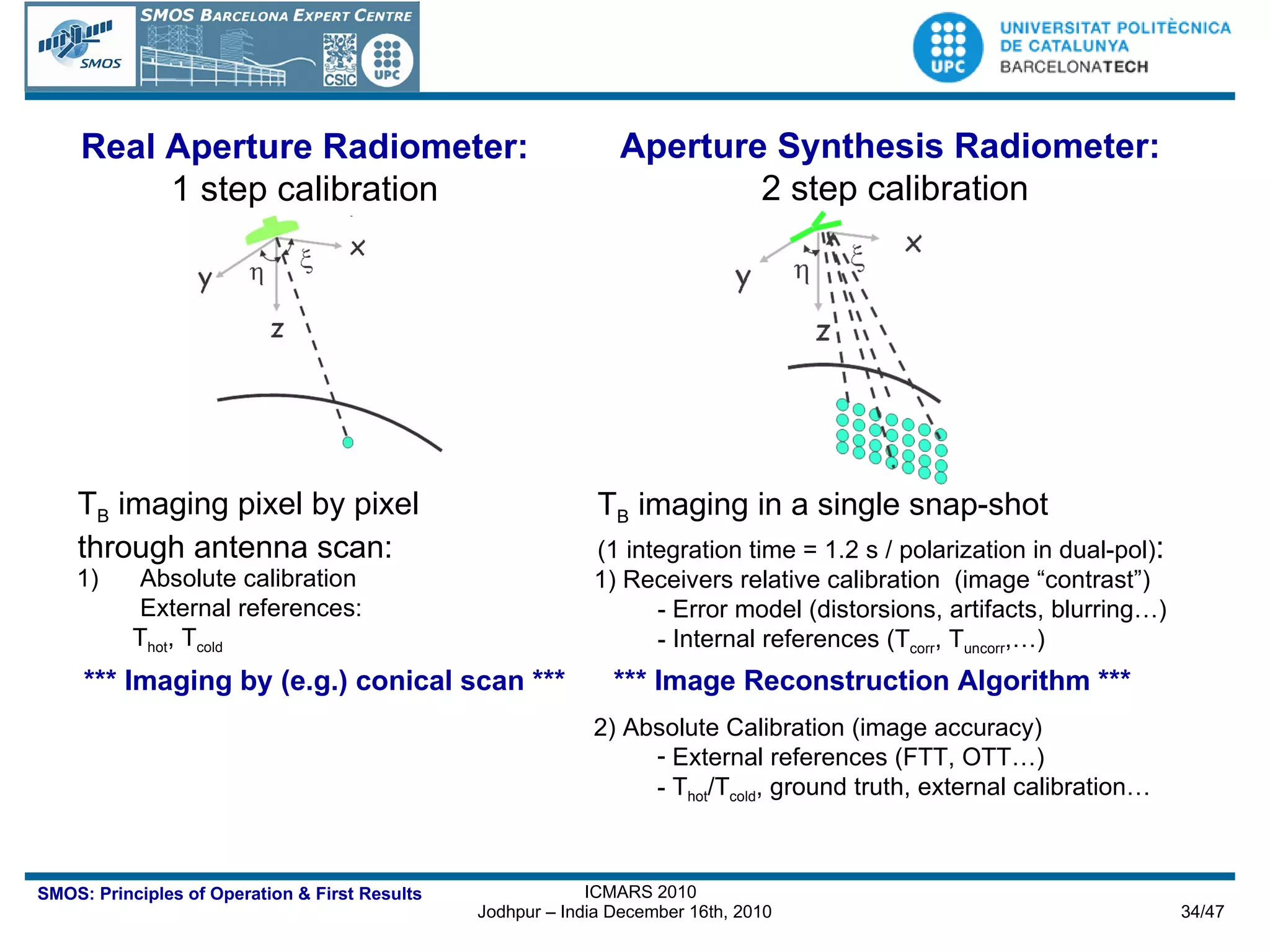
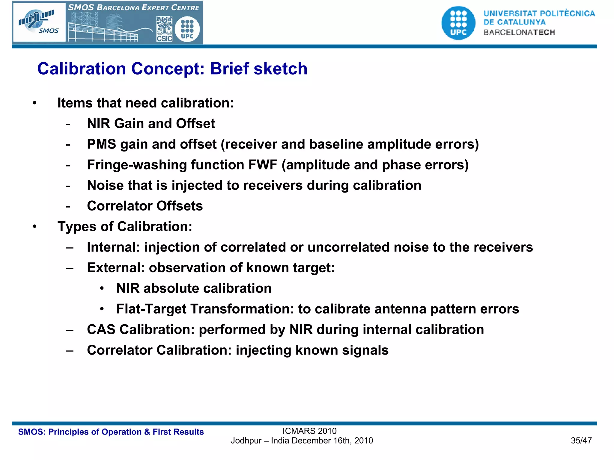
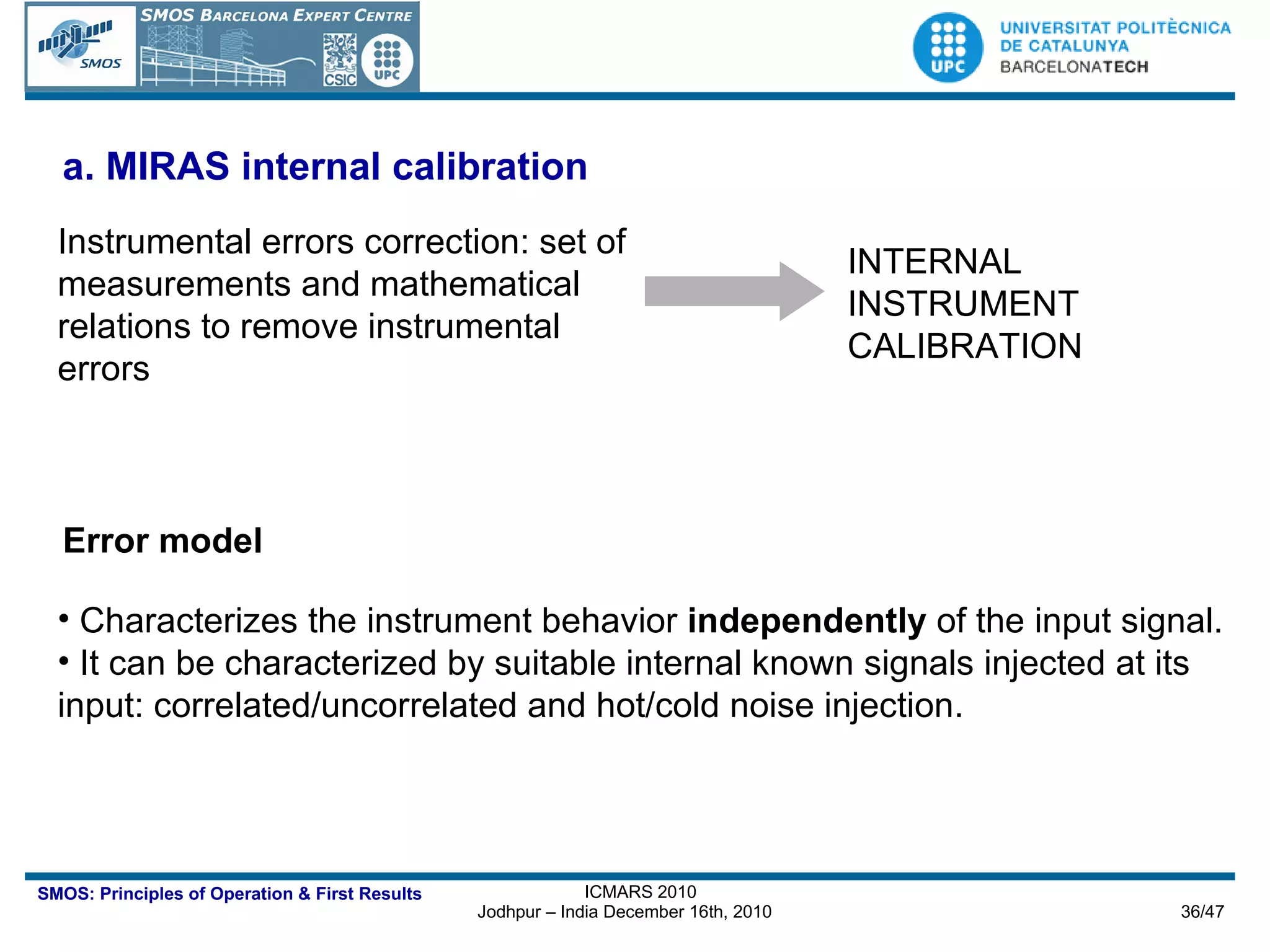
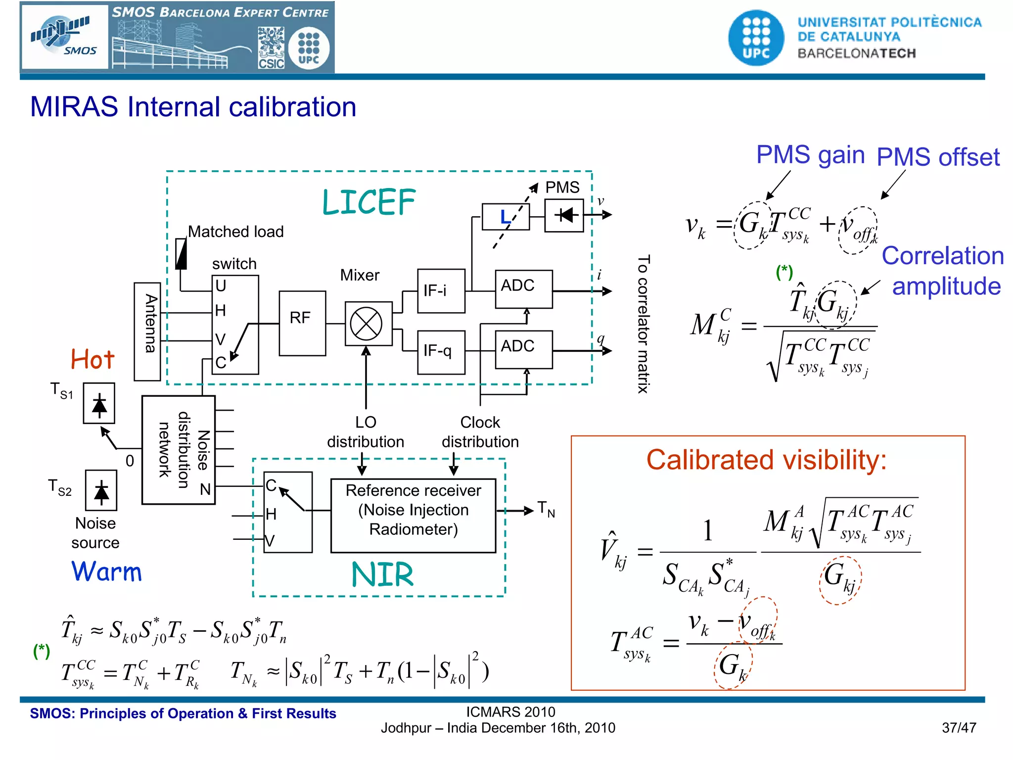
The document outlines the principles of operation of the Miras instrument used in the SMOS mission, detailing its imaging capabilities through synthetic aperture radiometry and the algorithms involved in image reconstruction. It describes the instrument's architecture, including its array topology, receiver systems, and calibration methods, as well as the performance metrics and geolocation techniques utilized for retrieving geophysical parameters. The importance of multi-angular observations and the precision required for accurate measurements of soil moisture and ocean salinity are emphasized throughout the document.
![SMOS: Principles of Operation of the MIRAS instrument Prof. A. Camps Dept. de Teoria del Senyal i Comunicacions Universitat Politècnica de Catalunya and IEEC/CRAE-UPC E-mail: [email_address] … on behalf of many people (many anonymous) that kept this dream alive and make it happen devoted to Prof. Cal Swift… the pioneer](https://image.slidesharecdn.com/icmars2010acamps-101213145349-phpapp01/75/MIRAS-the-instrument-aboard-SMOS-1-2048.jpg)
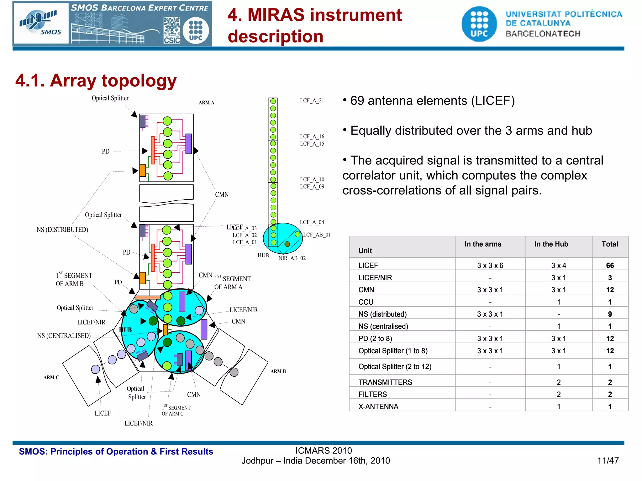
![MIRAS consists of a central structure (hub) with 15 elements, and 3 deployable arms, each one having 3 segments with 6 antennas each. [credits EADS-CASA]](https://image.slidesharecdn.com/icmars2010acamps-101213145349-phpapp01/75/MIRAS-the-instrument-aboard-SMOS-12-2048.jpg)
![LICEF: the LIght and Cost Effective Front-end [credits MIER Comunicaciones]](https://image.slidesharecdn.com/icmars2010acamps-101213145349-phpapp01/75/MIRAS-the-instrument-aboard-SMOS-14-2048.jpg)
![4.3. NIR architecture The Noise Injection Radiometer (NIR) is fully polarimetric and operates at 1.4 GHz 3 NIRs in the hub for redundancy. Functions: precise measurement of V pq (0,0) = T Apq for mean value of T Bpq ( , ) image. measurement of noise temperature level of the reference noise source of Calibration Subsystem (CAS) absolute amplitude reference 1 st LICEF unit (V-pol) 2 nd LICEF unit (H-pol) Controller unit (switches, noise injection...) Correlated noise inputs (from Noise Distribution Network) allow phase/amplitude calibration of receivers as LICEFs & for 3 rd and 4 th Stokes parameters measurements [credits TKK]](https://image.slidesharecdn.com/icmars2010acamps-101213145349-phpapp01/75/MIRAS-the-instrument-aboard-SMOS-15-2048.jpg)
![SMOS NIR: T NA + T A = T U T NA + T A = T REF + T NR Normal mode of operation: Calibrating internal noise source mode: known (cold sky) ? [Colliander et al., 2005] [credits HUT]](https://image.slidesharecdn.com/icmars2010acamps-101213145349-phpapp01/75/MIRAS-the-instrument-aboard-SMOS-16-2048.jpg)
![CCU: the Correlator and Control Unit [credits EADS-CASA]](https://image.slidesharecdn.com/icmars2010acamps-101213145349-phpapp01/75/MIRAS-the-instrument-aboard-SMOS-19-2048.jpg)
![OVERALL SEGMENT ARCHITECTURE [credits EADS-CASA]](https://image.slidesharecdn.com/icmars2010acamps-101213145349-phpapp01/75/MIRAS-the-instrument-aboard-SMOS-22-2048.jpg)
![[credits EADS-CASA] 6 LICEF / segment](https://image.slidesharecdn.com/icmars2010acamps-101213145349-phpapp01/75/MIRAS-the-instrument-aboard-SMOS-23-2048.jpg)
![[credits EADS-CASA] MOHA](https://image.slidesharecdn.com/icmars2010acamps-101213145349-phpapp01/75/MIRAS-the-instrument-aboard-SMOS-24-2048.jpg)
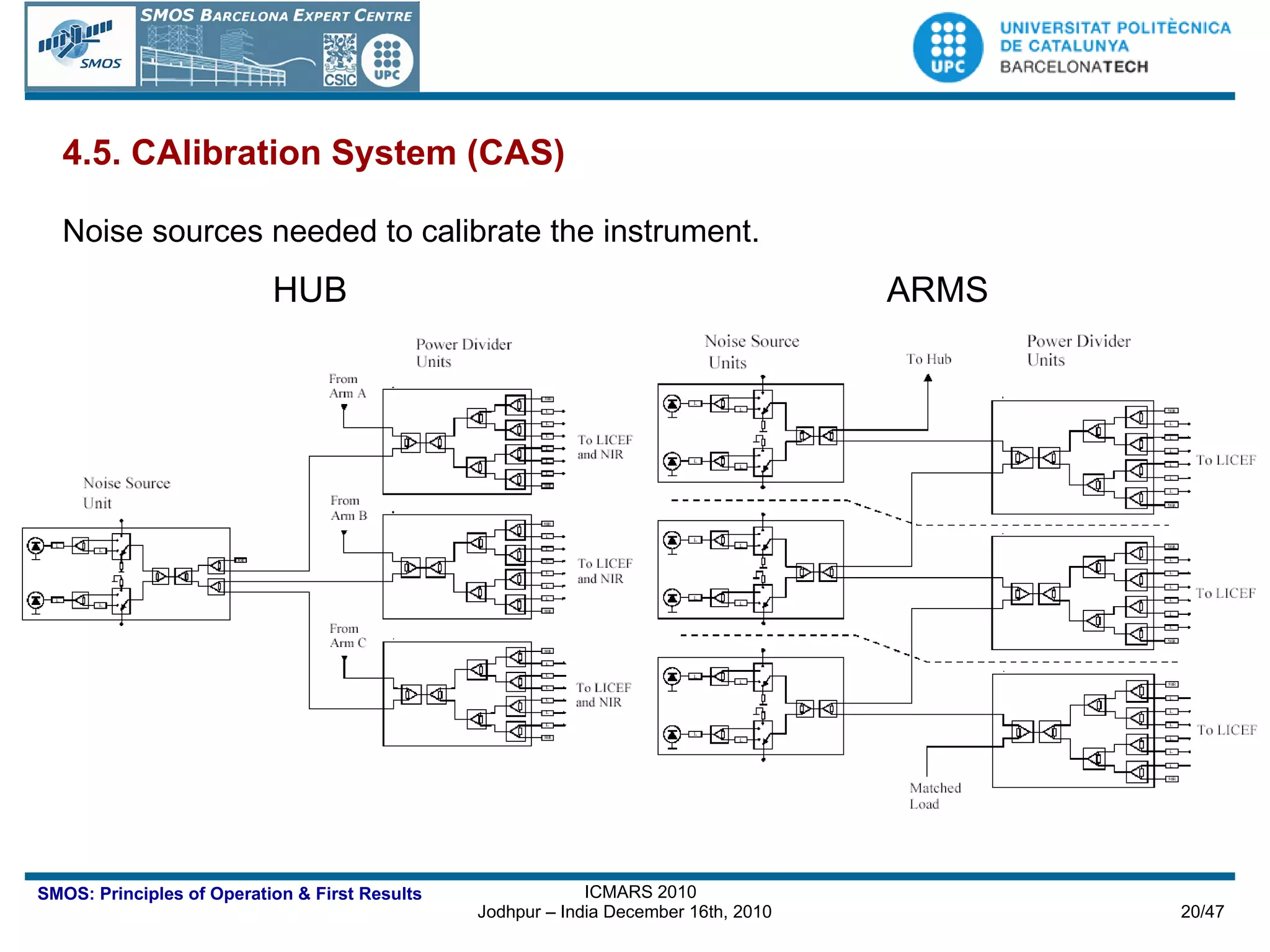
![[credits EADS-CASA] CAS](https://image.slidesharecdn.com/icmars2010acamps-101213145349-phpapp01/75/MIRAS-the-instrument-aboard-SMOS-25-2048.jpg)
![[credits EADS-CASA] CMN](https://image.slidesharecdn.com/icmars2010acamps-101213145349-phpapp01/75/MIRAS-the-instrument-aboard-SMOS-26-2048.jpg)
![Cut for =0 Dashed lines. Theoretical formula: Radiometric Sensitivity over ocean [credits I. Corbella]](https://image.slidesharecdn.com/icmars2010acamps-101213145349-phpapp01/75/MIRAS-the-instrument-aboard-SMOS-30-2048.jpg)
![Accuracy < 0.5 K Moon Galaxy (yellowish) Galaxy Alias Galactic radio-source (TBC) Cosmic Background Radiation at 3.3 K Sun Alias [credits DEIMOS] Scene Bias < 0.1 K](https://image.slidesharecdn.com/icmars2010acamps-101213145349-phpapp01/75/MIRAS-the-instrument-aboard-SMOS-31-2048.jpg)
![45 deg singularity discarded All points with the same incidence angle averaged Fresnel Incidence angle dependence Singularity in the transformation antenna to Earth reference frame (dual-pol mode) [credits I. Corbella]](https://image.slidesharecdn.com/icmars2010acamps-101213145349-phpapp01/75/MIRAS-the-instrument-aboard-SMOS-32-2048.jpg)
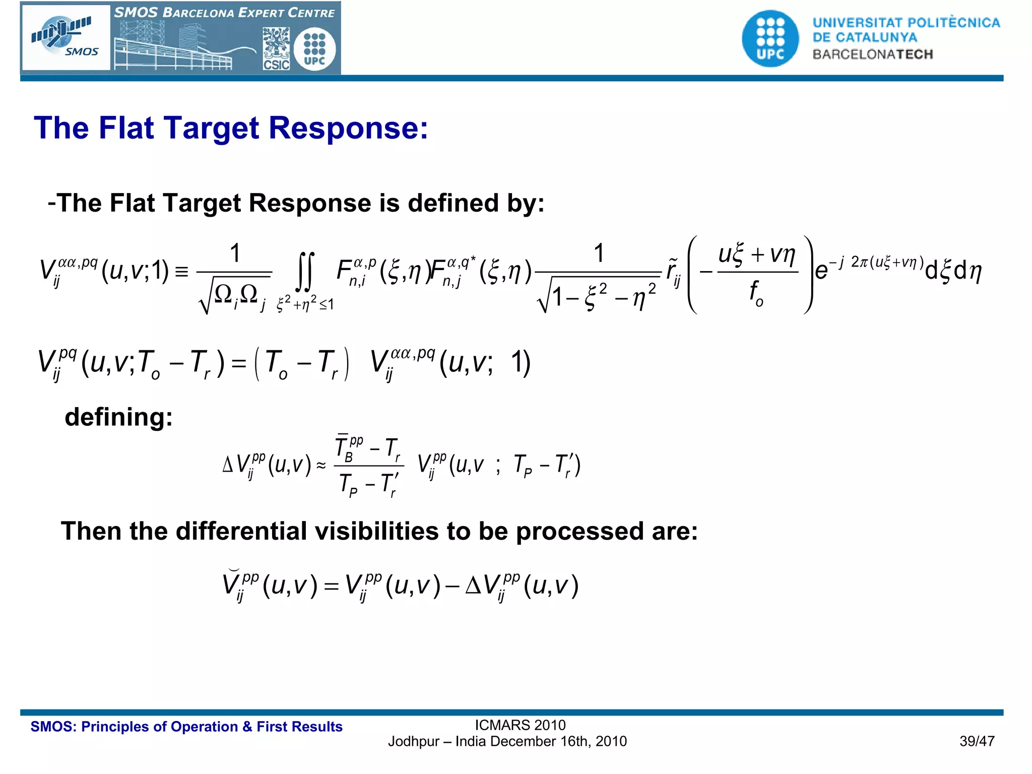
![Formulation of the Problem: Instrument Equation After Internal Calibration [credits I. Corbella] To be corrected using the Flat Target Response](https://image.slidesharecdn.com/icmars2010acamps-101213145349-phpapp01/75/MIRAS-the-instrument-aboard-SMOS-38-2048.jpg)
![Once in a month (every week during commissioning) the platform rotates to point to the cold sky External calibration is used to correct for elements not included in internal calibration: switch and antenna losses Also the Noise Injection Radiometer (NIR) is calibrated and the Flat Target Response (FTR) measured HERE IT GOES THE ANIMATION. T_X_skylook2.gif HERE IT GOES THE ANIMATION. T_Y_skylook2.gif External calibration [credits I. Corbella] Tx and Ty while satellite is turning up](https://image.slidesharecdn.com/icmars2010acamps-101213145349-phpapp01/75/MIRAS-the-instrument-aboard-SMOS-40-2048.jpg)
![5.4. Imaging Modes: Dual-polarization and full-polarimetric Dual-polarization radiometer: MIRAS has dual-pol antennas, but only one receiver polarizations have to be measured sequentially, with an integration time of 1.2 s each [credits M. Martin-Neira]](https://image.slidesharecdn.com/icmars2010acamps-101213145349-phpapp01/75/MIRAS-the-instrument-aboard-SMOS-41-2048.jpg)
![Full-polarimetric mode: (selected as operational mode for SMOS) [credits M. Martin-Neira]](https://image.slidesharecdn.com/icmars2010acamps-101213145349-phpapp01/75/MIRAS-the-instrument-aboard-SMOS-42-2048.jpg)
![Sample results of the application of the downscaling algorithm to a SMOS image covering the Murrumbidgee catchment, South-Eastern Australia, on January 19, 2010 (6 am). First row: 40 km SMOS soil moisture [m 3 /m 3 ] over Murrumbidgee (left), and zoom into Yanco site (right). Second row: 1 km downscaled soil moisture [m 3 /m 3 ] over Murrumbidgee (left), and zoom into Yanco site (right ). Dots indicate the location of the soil moisture permanent stations within the Murrumbidgee catchment used for validation purposes with colors representing their measurement at the exact SMOS acquisition time (only within Yanco site). Empty areas in the images correspond to non-retrieved soil moisture or clouds masking MODIS Ts measurements. (a) 60 x 60 km Yanco site in the Murrumbidgee catchment, South-Eastern Australia, (b) 1 km MODIS NDVI, and (c) and LST [K] on January 19, 2010. Sample SMOS data over Australia: Murrumbidge catchement 60 km (b) MODIS NDVI [m 3 /m 3 ] (c) MODIS LST [m 3 /m 3 ] (a) Murrumbidgee catchment 1 km downscaled SMOS soil moisture [m 3 /m 3 ] using MODIS VIS/IR data 40 km SMOS soil moisture [m 3 /m 3 ]](https://image.slidesharecdn.com/icmars2010acamps-101213145349-phpapp01/75/MIRAS-the-instrument-aboard-SMOS-46-2048.jpg)