The document discusses methods for estimating the distribution of species in a population using maximum likelihood estimation (MLE) and pattern maximum likelihood (PML) approaches, highlighting their applications in statistics, genetics, and system design. It critiques standard MLE for small sample sizes and proposes a non-parametric Poisson mixture model for better inference. Key results include the effectiveness of PML in accurately estimating probabilities and support sizes in various scenarios, including genomic applications.

1. A walk in the black
forest
Richard Gill

2. • Know nothing about mushrooms, can see if 2 mushrooms belong to
the same species or not
• S = set of all conceivable species of mushrooms
• n = 3, 3 = 2 + 1
• Want to estimate (functionals of) p = (ps : s ∈ S)
• S is (probably) huge
• MLE is ( ↦ 2/3, ↦ 1/3, “other” ↦ 0)
15:10 15:1215:42

3. Forget species names
(reduce data), then do MLE
• 3 = 2 + 1 is the partition of n = 3 generated by our sample =
reduced data
• qk := probability of k th most common species in population
• Estimate q = (q1, q2, …) (i.e., ps listed in decreasing order)
• Marginal likelihood = q1
2
q2 + q2
2
q1 + q1
2
q3 + q3
2
q1 + …
• Maximized by q = (1/2, 1/2, 0, 0, …) (exercise!)
• Many interesting functionals of p and of q = rsort(p) coincide
• But q = rsort(p) does not generally hold for MLE’s based on
reduced / all data, and many interesting functionals differ too

4. Examples
Acharya, Orlitsky, Pan (2009)
1000 = 6 x 7 + 2 x 6 + 17 x 5 + 51 x 4 + 86 x 3 + 138 x 2 + 123 x 1 (*)
0 200 400 600 800 1000
0.0001
0.0002
0.0005
0.0010
0.0020
0.0050 Naive estimator = !
full data MLE of q =!
rsort (full data MLE of p)!
!
Reduced data MLE of q!
!
True q
© (2014) Piet Groeneboom
(independent replication)
6 hrs, MH-EM, C.
104 outer EM steps.
106 inner MH to approximate
the E within each EM step
(*) Noncommutative multiplication: 6 x 7 = 6 species each observed 7 times)

5. estimate the un-
uality (1) bounds
y, JLm, is at least
JLm == 1 and all
actly one element
1122334. We call
+ 1) have PML
with the lemma,
a quasi-uniform
er m symbols.•
quasi-uniform and
e corollary yields
).
(1)
ISIr 2009, Seoul, Korea, June 28 - July 3, 2009
Canonical to P-;j) Reference
1 any distribution Trivial
11,111,111, ... (1) Trivial
12, 123, 1234, ... () Trivial
112,1122,1112,
(1/2, 1/2) [12]
11122, 111122
11223, 112233, 1112233 (1/3,1/3,1/3) [13]
111223, 1112223, (1/3,1/3,1/3) Corollary 5
1123, 1122334 (1/5,1/5, ... ,1/5) [12]
11234 (1/8,1/8, ... ,1/8) [13]
11123 (3/5) [15]
11112 (0.7887 ..,0.2113..) [12]
111112 (0.8322 ..,0.1678..) [12]
111123 (2/3) [15]
111234 (112) [15]
112234 (1/6,1/6, ... ,1/6) [13]
112345 (1/13, ... ,1/13) [13]
1111112 (0.857 ..,0.143..) [12]
1111122 (2/3, 1/3) [12]
1112345 (3/7) [15]
1111234 (4/7) [15]
1111123 (5/7) [15]
1111223 (1 0-1 0-1) Corollary 7
0' 20 ' 20
1123456 (1/19, ... ,1/19) [13]
1112234 (1/5,1/5, ... ,1/5)7 Conjectured
ISIT 2009, Seoul, Korea, June 28 - July 3, 2009
The Maximum Likelihood Probability of
Unique-Singleton, Ternary, and Length-7 Patterns
Jayadev Acharya
ECE Department, UCSD
Email: jayadev@ucsd.edu
Alon Orlitsky
ECE & CSE Departments, UCSD
Email: alon@ucsd.edu
Shengjun Pan
CSE Department, UCSD
Email: slpan@ucsd.edu
Abstract-We derive several pattern maximum likelihood
(PML) results, among them showing that if a pattern has only
one symbol appearing once, its PML support size is at most twice
the number of distinct symbols, and that if the pattern is ternary
with at most one symbol appearing once, its PML support size is
three. We apply these results to extend the set of patterns whose
PML distribution is known to all ternary patterns, and to all but
one pattern of length up to seven.
I. INTRODUCTION
Estimating the distribution underlying an observed data
sample has important applications in a wide range of fields,
including statistics, genetics, system design, and compression.
Many of these applications do not require knowing the
probability of each element, but just the collection, or multiset
of probabilities. For example, in evaluating the probability that
when a coin is flipped twice both sides will be observed, we
don't need to know p(heads) and p(tails), but only the multiset
{p( heads) ,p(tails) }. Similarly to determine the probability
that a collection of resources can satisfy certain requests, we
don't need to know the probability of requesting the individual
resources, just the multiset of these probabilities, regardless of
their association with the individual resources. The same holds
whenever just the data "statistics" matters.
One of the simplest solutions for estimating this proba-
bility multiset uses standard maximum likelihood (SML) to
find the distribution maximizing the sample probability, and
then ignores the association between the symbols and their
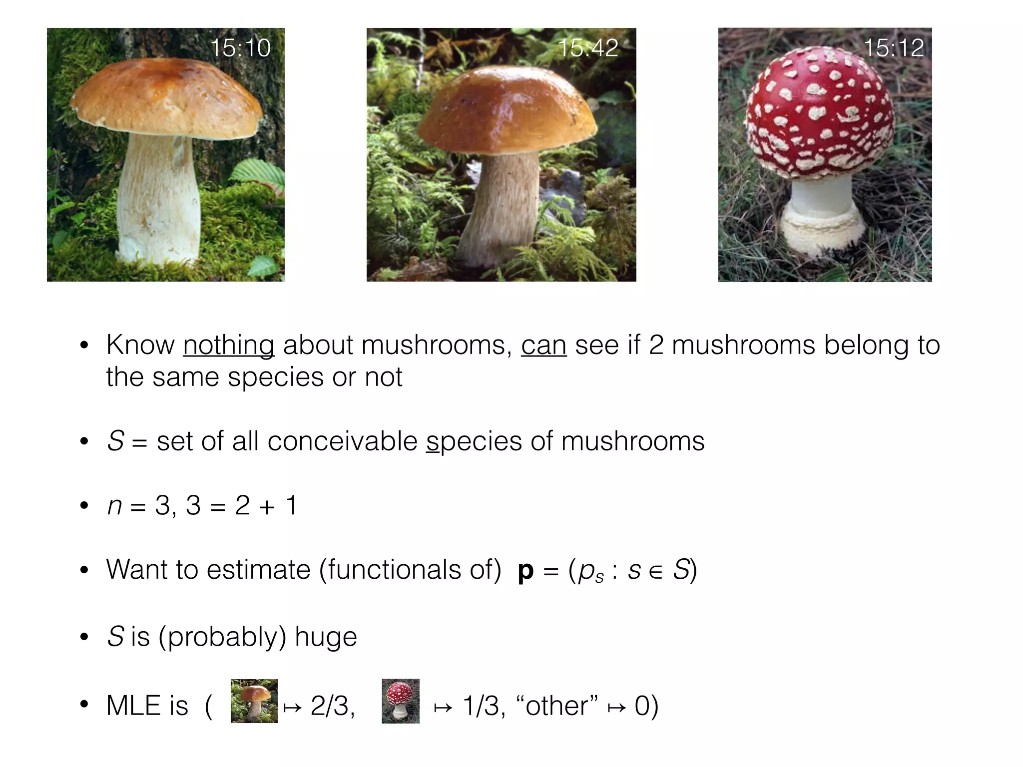
probabilities. For example, upon observing the symbols @ 1@,
SML would estimate their probabilities as p(@) == 2/3 and
p(1) == 1/3, and disassociating symbols from their probabili-
ties, would postulate the probability multiset {2/3, 1/3}.
SML works well when the number of samples is large
relative to the underlying support size. But it falls short when
the sample size is relatively small. For example, upon observ-
ing a sample of 100 distinct symbols, SML would estimate
a uniform multiset over 100 elements. Clearly a distribution
over a large, possibly infinite number of elements, would better
explain the data. In general, SML errs in never estimating a
support size larger than the number of elements observed, and
tends to underestimate probabilities of infrequent symbols.
Several methods have been suggested to overcome these
problems. One line of work began by Fisher [1], and was
followed by Good and Toulmin [2], and Efron and Thisted [3].
Bunge and Fitzpatric [4] provide a comprehensive survey of
many of these techniques.
A related problem, not considered in this paper estimates the
probability of individual symbols for small sample sizes. This
problem was considered by Laplace [5], Good and Turing [6],
and more recently by McAllester and Schapire [7], Shamir [8],
Gemelos and Weissman [9], Jedynak and Khudanpur [10], and
Wagner, Viswanath, and Kulkarni [11].
A recent information-theoretically motivated method for the
multiset estimation problem was pursued in [12], [13], [14]. It
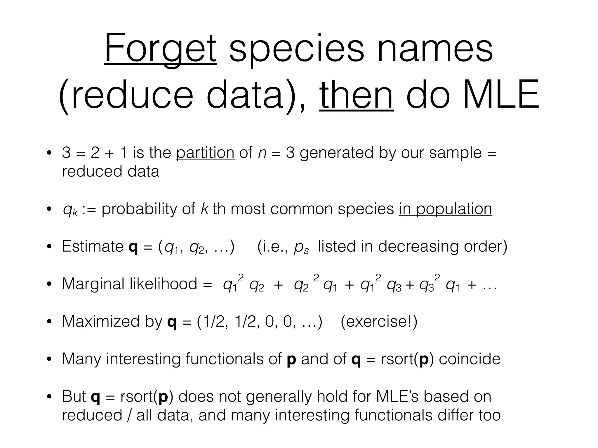
is based on the observation that since we do not care about the
association between the elements and their probabilities, we
can replace the elements by their order of appearance, called
the observation's pattern. For example the pattern of @ 1 @ is
121, and the pattern of abracadabra is 12314151231.
Slightly modifying SML, this pattern maximum likelihood
(PML) method asks for the distribution multiset that maxi-
mizes the probability of the observed pattern. For example,
the 100 distinct-symbol sample above has pattern 123...100,
and this pattern probability is maximized by a distribution
over a large, possibly infinite support set, as we would expect.
And the probability of the pattern 121 is maximized, to 1/4,
by a uniform distribution over two symbols, hence the PML
distribution of the pattern 121 is the multiset {1/2, 1/2} .
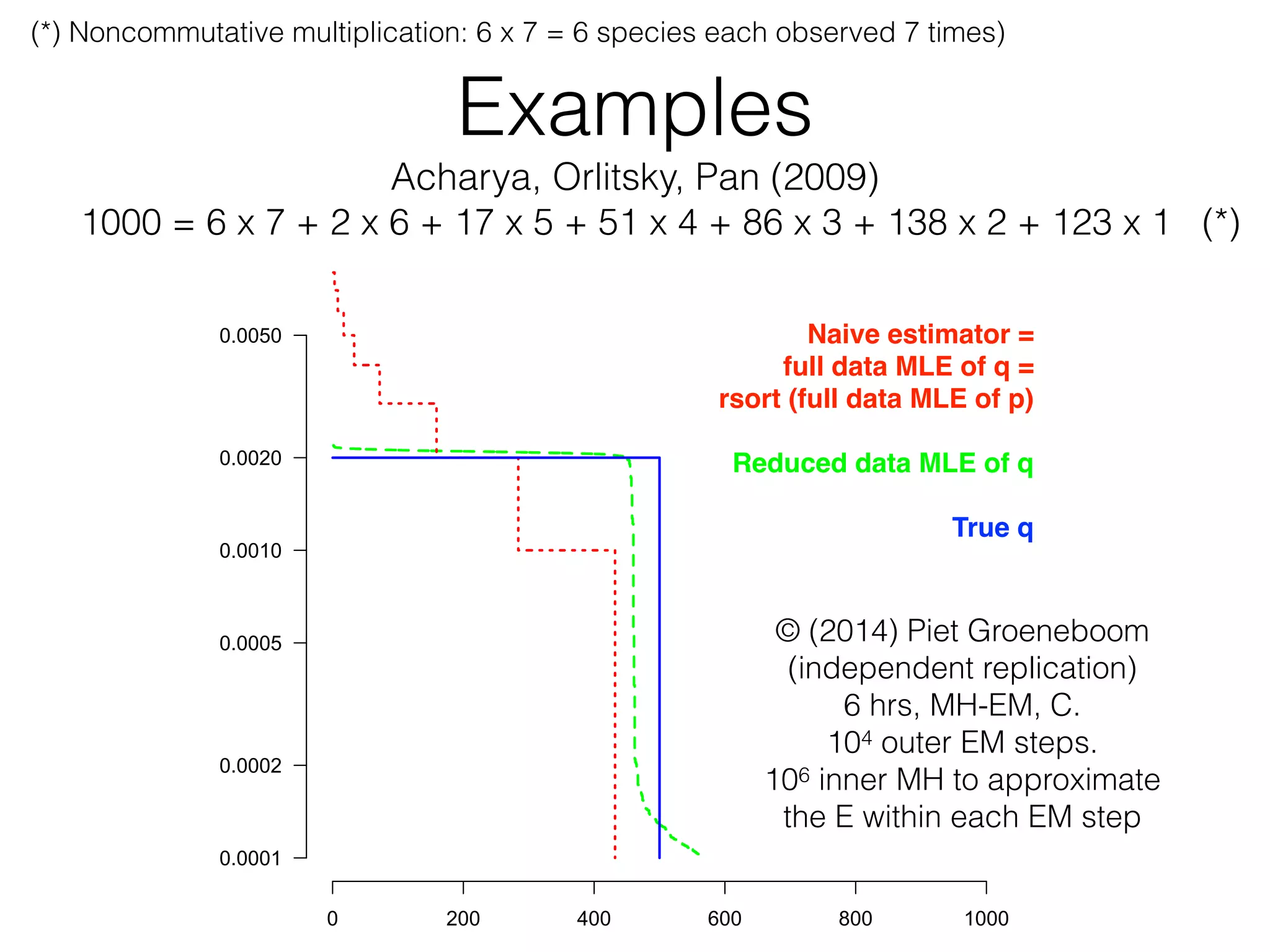
To evaluate the accuracy of PML we conducted the fol-
lowing experiment. We took a uniform distribution over 500
elements, shown in Figure 1 as the solid (blue) line. We sam-
pled the distribution with replacement 1000 times. In a typical
run, of the 500 distribution elements, 6 elements appeared 7
times, 2 appeared 6 times, and so on, and 77 did not appear at
all as shown in the figure. The standard ML estimate, which
always agrees with empirical frequency, is shown by the dotted
(red) line. It underestimates the distribution's support size by
over 77 elements and misses the distribution's uniformity. By
contrast, the PML distribution, as approximated by the EM
algorithm described in [14] and shown by the dashed (green)
line, performs significantly better and postulates essentially the
correct distribution.
As shown in the above and other experiments, PML's
empirical performance seems promising. In addition, several
results have proved its convergence to the underlying distribu-
tion [13], yet analytical calculation of the PML distribution for
specific patterns appears difficult. So far the PML distribution
has been derived for only very simple or short patterns.
Among the simplest patterns are the binary patterns, con-
sisting of just two distinct symbols, for example 11212. A
formula for the PML distributions of all binary patterns was
978-1-4244-4313-0/09/$25.00 ©2009 IEEE 1135
7 = 3 + 2 + 1 + 1
5 = 3 + 1 + 1
1 = 1!
n = n (= 2, 3, …)!
n = 1 + 1 + 1 + …

6. frequency 27 23 16 14 13 12 11 10 9 8 7 6 5 4 3 2 1
replicates 1 1 2 1 1 1 2 2 1 3 2 6 11 33 71 253 1434
Biometrika(2002), 89, 3, pp.669-681
? 2002 Biometrika Trust
Printedin GreatBritain
A Poisson model for the coverageproblemwith a genomic
application
BY CHANG XUAN MAO
InterdepartmentalGroupinBiostatistics, Universityof California,Berkeley,
367 EvansHall, Berkeley,California94720-3860, U.S.A.
cmao@stat.berkeley.edu
AND BRUCE G. LINDSAY
Departmentof Statistics, PennsylvaniaState University,UniversityPark,
Pennsylvania16802-2111, U.S.A.
bgl@psu.edu
SUMMARY
Suppose a population has infinitely many individuals and is partitioned into unknown
N disjoint classes. The sample coverage of a random sample from the population is the
total proportion of the classes observed in the sample. This paper uses a nonparametric
Poisson mixture model to give new understanding and results for inference on the sample
coverage. The Poisson mixture model provides a simplified framework for inferring any
generalabundance-f coverage, the sum of the proportions of those classes that contribute
exactly k individuals in the sample for some k in *, with * being a set of nonnegative
integers. A new moment-based derivation of the well-known Turing estimators is pre-
sented.As an application, a gene-categorisation problem in genomic researchis addressed.
Since Turing'sapproach is a moment-based method, maximum likelihood estimation and
minimum distance estimation are indicated as alternatives for the coverage problem.
Finally, it will be shown that any Turing estimator is asymptotically fully efficient.
Somekey words:Digital gene expression;Poisson mixture;Sample coverage; Species.
1. INTRODUCTION
Consider a population composed of infinitelymany individuals, which can be considered
as an approximation of real populations with finitely many individuals under specific situ-
ations, in particular when the number of individuals in a target population is very large.
The population has been partitioned into N disjoint classes indexed by i=1,2,..., N,
with ic being the proportion of the ith class. The identity of each class and the parameter
N are assumed to be unknown prior to the experiment. The unknown m,'sare subject to
the constraint 7~•{1 = 1. A random sample of individuals is taken from the population.
Let X, be the number of individuals from the ith class, called the frequency in the sample.
If X, = 0, then the ith class is not observed in the sample. It will be assumed that these
zero frequencies are 'missed' random variables so that N, the 'sample size' of all the Xi's,
is unknown. Let nk be the number of classes with frequency k and s be the number of
A Poisson model for the coverageproblemwith a genomic
application
BY CHANG XUAN MAO
InterdepartmentalGroupinBiostatistics, Universityof California,Berkeley,
367 EvansHall, Berkeley,California94720-3860, U.S.A.
cmao@stat.berkeley.edu
AND BRUCE G. LINDSAY
Departmentof Statistics, PennsylvaniaState University,UniversityPark,
Pennsylvania16802-2111, U.S.A.
bgl@psu.edu
SUMMARY
Suppose a population has infinitely many individuals and is partitioned into unknown
N disjoint classes. The sample coverage of a random sample from the population is the
total proportion of the classes observed in the sample. This paper uses a nonparametric
Poisson mixture model to give new understanding and results for inference on the sample
coverage. The Poisson mixture model provides a simplified framework for inferring any
generalabundance-f coverage, the sum of the proportions of those classes that contribute
exactly k individuals in the sample for some k in *, with * being a set of nonnegative
integers. A new moment-based derivation of the well-known Turing estimators is pre-
sented.As an application, a gene-categorisation problem in genomic researchis addressed.
Since Turing'sapproach is a moment-based method, maximum likelihood estimation and
minimum distance estimation are indicated as alternatives for the coverage problem.
Finally, it will be shown that any Turing estimator is asymptotically fully efficient.
Somekey words:Digital gene expression;Poisson mixture;Sample coverage; Species.
1. INTRODUCTION
Consider a population composed of infinitelymany individuals, which can be considered
as an approximation of real populations with finitely many individuals under specific situ-
ations, in particular when the number of individuals in a target population is very large.
The population has been partitioned into N disjoint classes indexed by i=1,2,..., N,
with ic being the proportion of the ith class. The identity of each class and the parameter
N are assumed to be unknown prior to the experiment. The unknown m,'sare subject to
the constraint 7~•{1 = 1. A random sample of individuals is taken from the population.
Let X, be the number of individuals from the ith class, called the frequency in the sample.
If X, = 0, then the ith class is not observed in the sample. It will be assumed that these
zero frequencies are 'missed' random variables so that N, the 'sample size' of all the Xi's,
is unknown. Let nk be the number of classes with frequency k and s be the number of
– naive
– mle
– naive!
– mle
LR = 2200!
!
LR = 7400!
Good-Turing = 7300
N = 2586; 21 x 106 iterations of SA-MH-EM (24 hrs) (right panel: y-axis logarithmic)
ˆ
ˆ
(mle has mass 0.3 spread thinly beyond 2000 – for optimisation, taken infinitely thin, inf. far)
Tomato genes ordered by frequency of expression
qk = probability gene k is being expressed
Very similar to typically Y-STR haplotype data!
0 500 1000 1500 2000
0.0000.0020.0040.0060.0080.010
0 500 1000 1500 2000
1e−042e−045e−041e−032e−035e−031e−02
© (2014) Richard Gill
R / C++ using Rcpp interface
MH and EM steps alternate,
E updated by SA =
“stochastic approximation”

7. The Fundamental Problem of Forensic Statistics
(Sparsity, and sometimes Less is More)
Richard Gill
with: Dragi Anevski, Stefan Zohren;
Michael Bargpeter; Giulia Cereda
September 12, 2014

8. Data (database):
X ∼ Multinomial(n, p) p = (ps : s ∈ S)
#S is huge (all theoretically possible species)
Very many ps are very small, almost all are zero
Conventional task:
Estimate ps, for a certain s such that Xs = 0
Preferably, also inform “consumer” of accuracy
At present hardly ever known, hardly ever done

9. Motivation:
Each “species” = a possible DNA profile
We have a database of size n of a sample of DNA profiles
e.g. Y-chromosome 8 locus STR haplotypes (yhrd.org)
e.g. Mitochondrial DNA, ...
Some profiles occur many times, some are very rare,
most “possible” profiles do not occur in the data-base at all
Profile s is observed at a crime-scene
We have a suspect and his profile matches
We never saw s before, so it must be rare
Likelihood ratio (prosecution : defence) is 1/ps
Evidential value is − log10(ps) ban’s
(one ban = 2.30 nats = 3.32 bits)

10. Present day practices
Type 1: don’t use any prior information, discard most data
Various ad-hoc “elementary” approaches
No evaluation of accuracy
Type 2: use all prior information, all data
Model (ps : s ∈ S) using population genetics, biology, imagination:
Hierarchy of parametric models of rapidly increasing complexity:
“Present day population equals finite mixture of subpopulations
each following exact theoretical law”.
e.g. Andersen et al. (2013) “DiscLapMix”:
Model selection by AIC, estimation by EM (MLE), plug-in for LR
No evaluation of accuracy
Both types are (more precisely: easily can be) disastrous

11. New approach: Good-Turing
Idea 1: full data = database + crime scene + suspect data
Idea 2: reduce full data cleverly to reduce complexity,
to get better-estimable and better-evaluable LR without losing
much discriminatory power
Database & all evidence together = sample of size n, twice
increased by +1
Reduce complexity by forgetting names of the species
All data together is reduced to
partition of n implied by database, together with
partition of n + 1 (add crime-scene species to database)
partition of n + 2 (add suspect species to database)
Database partition = spectrum of database species frequencies
= Y = rsort(X) (reverse sort)

12. The distribution of database frequency spectrum Y = rsort(X)
only depends on q = rsort(p)
the spectrum of true species probabilities (*)
Note: components of X and of p are indexed by s ∈ S,
components of Y and of q are indexed by k ∈ N+,
Y/n (database spectrum, expressed as relative frequencies)
is for our purposes a lousy estimator of q
(i.e., for the functionals of q we are interested in),
even more so than X/n is a lousy estimator of p (for those
functionals)
(*) More generally, (joint) laws of (Y, Y+, Y++) under prosecution and
defence hypotheses only depend on q

13. Our aim: estimate reduced data LR
LR = s∈S(1 − ps)nps
s∈S(1 − ps)np2
s
= k∈N+ (1 − qk)nqk
k∈N+ (1 − qk)nq2
k
or, “estimate” reduced data conditional LR
LRcond = s∈S I{Xs = 0}qs
s∈S I{Xs = 0}q2
s
and report (or at the least, know something about) the precision of
the estimate
Important to transform to “bans” (ie take negative log base 10)
before discussing precision

14. Key observations
Database spectrum can be reduced to Nx = #{s : Xs = x},
x ∈ N+, or even further, to {(x, Nx ) : Nx > 0}
Add superscript n to “impose” dependence on sample size,
n + 1
1
s∈S
(1 − ps)n
ps = En+1
(N1) ≈ En
(N1)
n + 2
2
s∈S
(1 − ps)n
p2
s = En+2
(N2) ≈ En
(N2)
suggests: estimate LR (or LRcond!) from database by
nN1
2N2
Alternative: estimate by plug-in of database MLE of q in formula
for LR as function of q
But how accurate is LR?

15. Accuracy (1): asymptotic normality; wlog S = N+, p = q
Poissonization trick: pretend n is realisation of N ∼ Poisson(λ)
=⇒ Xs ∼ independent Poisson(λps)
(N, N1, N2) = s(Xs, I{Xs = 1}, I{Xs = 2}) should be
asymptotically Gaussian3 as λ → ∞
Conditional law of (N1, N2) given N = n = λ → ∞, hopefully,
converges to corresponding conditional Gaussian2
Proof: Esty (1983), no N2, p depending on n,
√
n normalisation;
Zhang & Zhang (2009): N&SC, implying p must vary with n to
have convergence (& non degenerate limit) at this rate.
Conjecture: Gaussian limit with slower rate and fixed p possible,
under appropriate tail behaviour of p; rate will depend on tail
“exponent” (rate of decay of tail)
Formal delta-method calculations give simple conjectured
asymptotic variance estimator depending on n, N1, N2, N3, N4;
simulations suggest “it works”

16. Accuracy (2): MLE and bootstrap
Problem: Nx gets rapidly unstable as x increases
Good & Turing proposed “smoothing” the higher observed Nx
Alternative: Orlitsky et al. (2004, 2005, ...): estimate q by MLE
Likelihood = k qYk
χ(k), sum over bijections χ : N+ → N+
Anevksy, Gill, Zohren (arXiv:1312.1200) prove (almost) root n
L1-consistency by delicate proof based on simple ideas inspired by
Orlitsky (et al.) “outline” of “proof”
Must “close” parameter space to make MLE exist – allow positive
probability “blob” of zero probability species
Computation: SA-MH-EM
Proposal: use database MLE to estimate accuracy (bootstrap),
and possibly to give alternative estimator of LR

17. Open problems
(1) Get results for these and other interesting functionals of MLE,
e.g., entropy
Conjecture: will see interesting convergence rates depending on
rate of decay of tail of q
Conjecture: interesting / useful theorems require q to depend on n
Problems of adaptation, coverage probability challenges
(2) Prove “semiparametric” bootstrap works for such functionals
(3) Design computationally feasible nonparametric Bayesian
approach (a confidence region for a likelihood ratio is an oxymoron)
and verify it has good frequentist properties;
or design hybrid (i.e., “empirical Bayes”) approaches = Bayes with
data-estimated hyperparameter

18. Remarks
Plug-in MLE to estimate E(Nx ) almost exactly reproduces observed
Nx : order of size of sqrt(expected) minus sqrt(observed) is ≈ ±1
2
Our approach is all the more useful when case involves match of a
not new but still (in database) uncommon species:
Good-Turing-inspired estimated LR easy to generalise, involves Nx
for“higher” x, hence better to smooth by replacing with MLE
predictions / estimation of expectations

19. Consistency proof

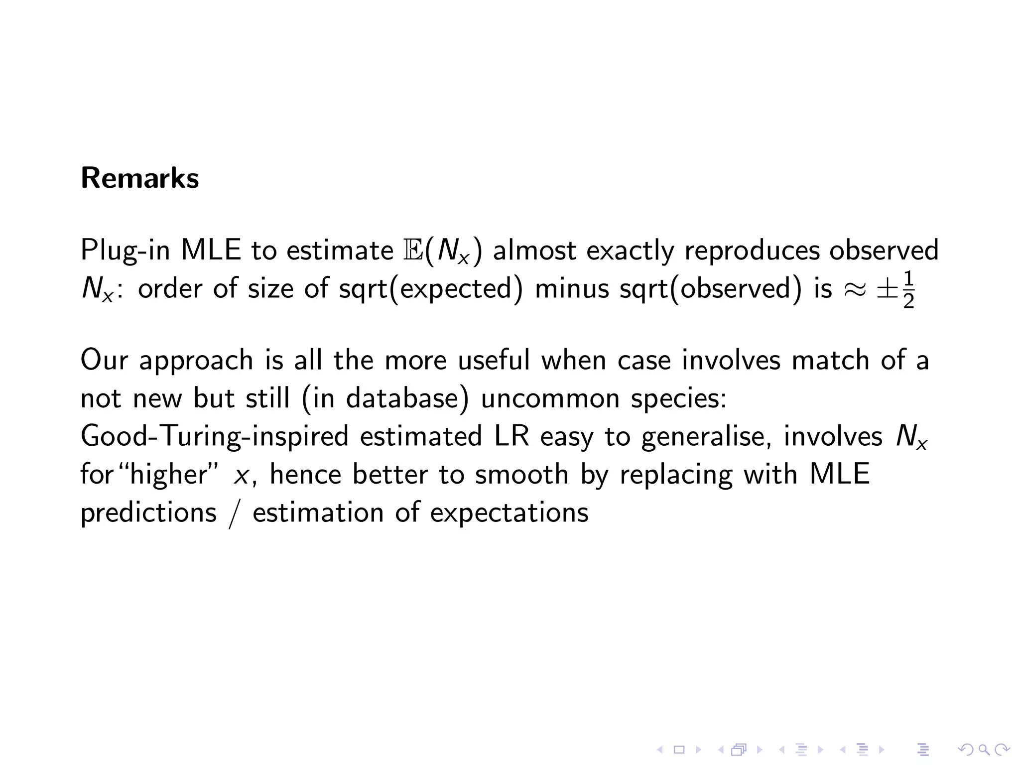
20. • Convergence at rate n – (k – 1) / 2k if 𝜃x ≈ C / x k
• Convergence at rate n – 1 / 2 if 𝜃x ≈ A exp( – B x k)
Estimating a probability mass function with
unknown labels
Dragi Anevski, Richard Gill, Stefan Zohren,
Lund University, Leiden University, Oxford University
July 25, 2012 (last revised DA, 10:10 am CET)
Abstract
1 The model
1.1 Introduction
Imagine an area inhabited by a population of animals which can be classified
by species. Which species actually live in the area (many of them previously
unknown to science) is a priori unknown. Let A denote the set of all possible
species potentially living in the area. For instance, if animals are identified by
their genetic code, then the species’ names ↵ are “just” equivalence classes
of DNA sequences. The set of all possible DNA sequences is e↵ectively
uncountably infinite, and for present purposes so is the set of equivalence
classes, each equivalence class defining one “potential” species.
Suppose that animals of species ↵ 2 A form a fraction ✓↵ 0 of the total
population of animals. The probabilities ✓ are completely unknown.
Corollary:
14 ANEVSKI, GILL AND ZOHREN
We show that an extended maximum likelihood estimator exists in Ap-
pendix A of [3]. We next derive the almost sure consistency of (any) extended
maximum likelihood estimator ˆ✓.
Theorem 1. Let ˆ✓ = ˆ✓(n) be (any) extended maximum likelihood esti-
mator. Then for any > 0
Pn,✓
(||ˆ✓ ✓||1 > ) 
1
p
3n
e⇡
p2n
3
n ✏2
2 (1 + o(1)) as n ! 1
where ✏ = /(8r) and r = r(✓, ) such that
P1
i=r+1 ✓i  /4.
Proof. Now let Q✓, be as in the statement of Lemma 1. Then there is
an r such that the conclusion of the lemma holds, i.e. for each n there is a
set
A = An = { sup
1xr
| ˆf(n)
x ✓x|  ✏}
such that
n,✓ n✏2/2

21. Tools
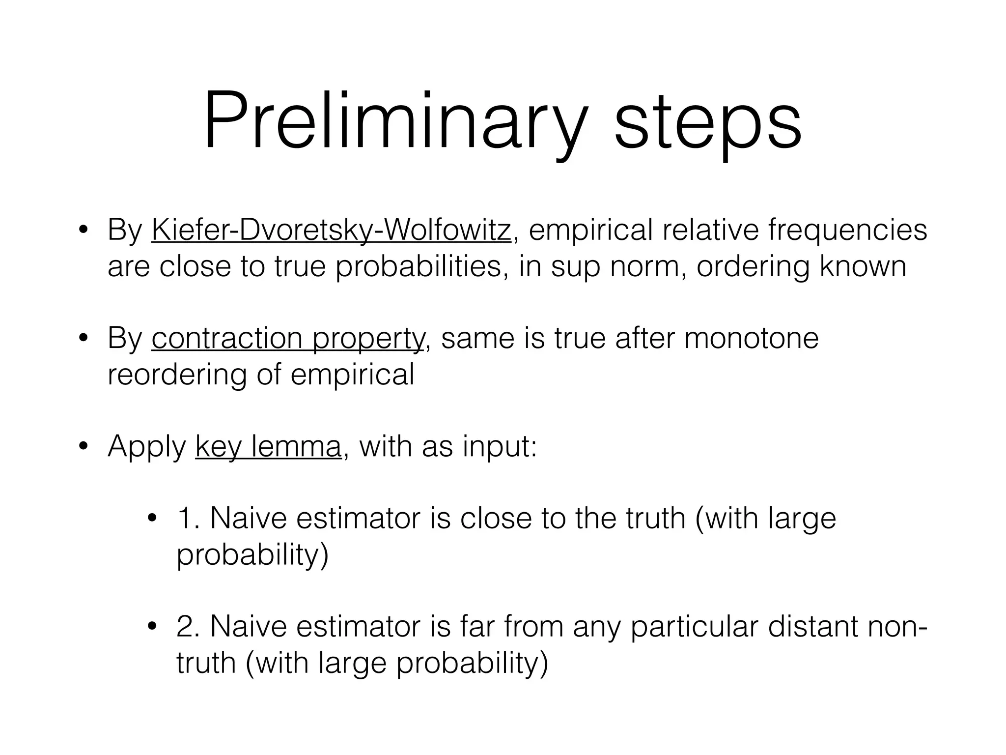
• Kiefer-Dvoretsky-Wolfowitz
• “r-sort” is contraction mapping w.r.t sup norm
• Hardy-Ramanujan: number of partitions of n grows as
ESTIMATING A PROBABILITY MASS FUNCTION 15
is an extended ML estimator then
dPn,ˆ✓
dPn,✓
1.
a given n = n1 + . . . + nk such that n1 . . . nk > 0, (with k varying),
re is a finite number p(n) of possibilities for the value of (n1, . . . , nk). The
mber p(n) is the partition function of n, for which we have the asymptotic
mula
p(n) =
1
4n
p
3
e⇡
p2n
3 (1 + o(1)),
n ! 1, cf. [23]. For each possibility of (n1, . . . , nk) there is an extended
estimator (for each possibility we can choose one such) and we let Pn =
From (8) follows that for some i  r we have
|✓i i|
4r
:= 2✏ = 2✏( , ✓).)
ote that r, and thus also ✏ depends only on ✓, and not on .
Recall the Dvoretzky-Kiefer-Wolfowitz (DKW) inequality [6, 17]; for e
> 0
P✓(sup
x 0
|F(n)
(x) F✓(x))| ✏)  2e 2n✏2
,0)
here F✓ is the cumulative distribution function corresponding to ✓,
(n) the empirical probability function based on i.i.d. data from F✓.
upx 0 |F(n)(x) F✓(x)| ✏} {supx 0 |f
(n)
x ✓x| 2✏} {supx 1 |f
| 2✏}, with f(n) the empirical probability mass function correspon
F(n), equation (10) implies
Pn,✓
(sup
x 1
|f(n)
x ✓x| ✏) = P✓(sup
x 1
|f(n)
x ✓x| ✏)
r-sort = reverse sort = sort in decreasing order

22. Key lemma
P, Q probability measures; p, q densities
• Find event A depending on P and 𝛿
• P (Ac) ≤ 𝜀
• Q (A) ≤ 𝜀 for all Q: d (Q, P) ≥ 𝛿
• Hence P ( p /q < 1) ≤ 2𝜀 if d (Q, P) ≥ 𝛿
Application:
P, Q are probability distributions of data,
depending on parameters 𝜃, 𝜙 respectively
A is event that Y/n is within 𝛿 of 𝜃 (sup norm)
d is L1 distance between 𝜃 and 𝜙
Proof:
P ( p /q < 1)
= P( p /q < 1 ∩ Ac) + P( p /q < 1 ∩ A)
≤ P(Ac) + Q(A)

23. Preliminary steps
• By Kiefer-Dvoretsky-Wolfowitz, empirical relative frequencies
are close to true probabilities, in sup norm, ordering known
• By contraction property, same is true after monotone
reordering of empirical
• Apply key lemma, with as input:
• 1. Naive estimator is close to the truth (with large
probability)
• 2. Naive estimator is far from any particular distant non-
truth (with large probability)

24. Proof outiline
• By key lemma, probability MLE is any particular q
distant from (true) p is very small
• By Hardy, there are not many q to consider
• Therefore probability MLE is far from p is small
• Careful – sup norm on data, L1 norm on parameter
space, truncation of parameter vectors ...

25. –Ate Kloosterman
A practical question from the NFI:
It is a Y-chromosome identification case (MH17 disaster).
A nephew (in the paternal line) of a missing male individual and the unidentified victim share the
same Y-chromosome haplotype.
The evidential value of the autosomal DNA evidence for this ID is low (LR=20).
The matching Y-str haplotype is unique in a Dutch population sample (N=2085) and in the
worldwide YHRD Y-str database (containing 84 thousand profiles).
I know the distribution of the haplotype frequencies in the Dutch database (1826 haplotypes)
Distribution of haplotype frequencies
Database frequency of haplotype 1 2 3 4 5 6 7 13
Number of haplotypes in database 1650 130 30 7 5 2 1 1

26. N = 2085; 106 x 105 (outer x inner) iterations of SA-MH-EM (12 hrs) (y-axis logarithmic)
mle puts mass 0.51 spread thinly beyond 2500 – for optimisation, taken infinitely thin, inf. far
© (2014) Richard Gill
R / C++ using Rcpp interface
outer EM and inner MH steps
E updated by SA =
“stochastic approximation”
Estimated NL Y-str haplotype probability distribution
0 500 1000 1500 2000 2500
0.000050.000200.000500.002000.00500
Haplotype
Probability
PML
Naieve
Initial (1/200 sqrt x)

27. Observed and expected number of haplotypes, by database frequency
Frequency 1 2 3 4 5 6
O 1650 130 30 7 5 2
E 1650.49 129.64 29.14 8.99 3.77 1.75
Hanging rootogram
Database frequency
−1.0−0.50.00.51.0

28. Bootstrap s.e. 0.040, Good-Turing asymptotic theory estimated s.e. 0.044
4.00 4.05 4.10 4.15 4.20 4.25
0246810
Bootstrap distribution of Good−Turing log10LR
Bootstrap log10LR
Probabilitydensity