Downloaded 43 times


![Quantum key distribution [BB’84]
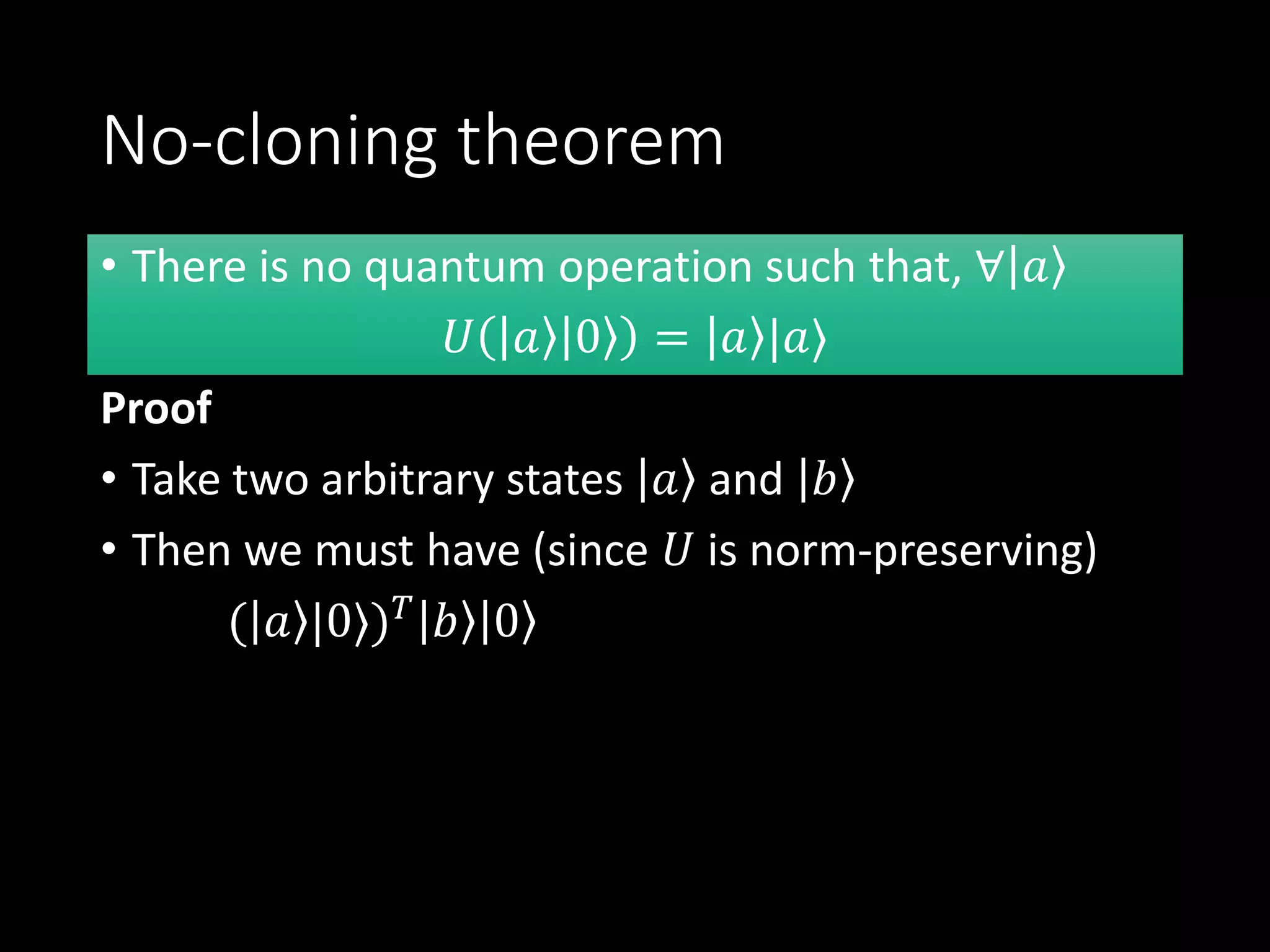
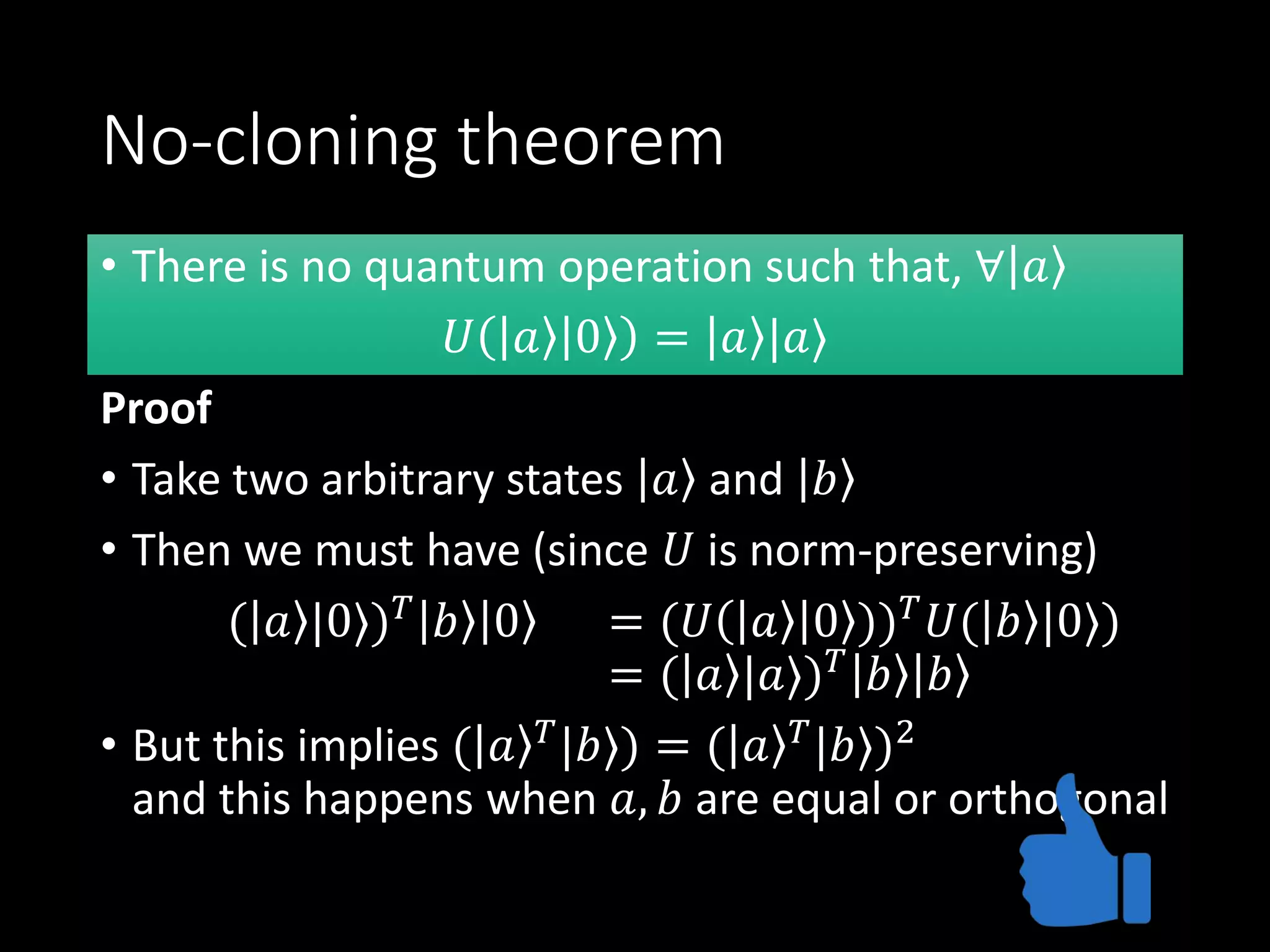
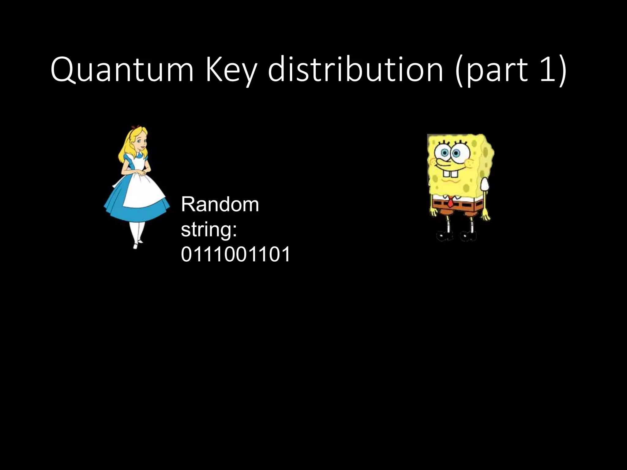
• Alice & Bob want to establish a secret key
• They communicate through a public quantum
channel
• They make use of the following 2 facts:
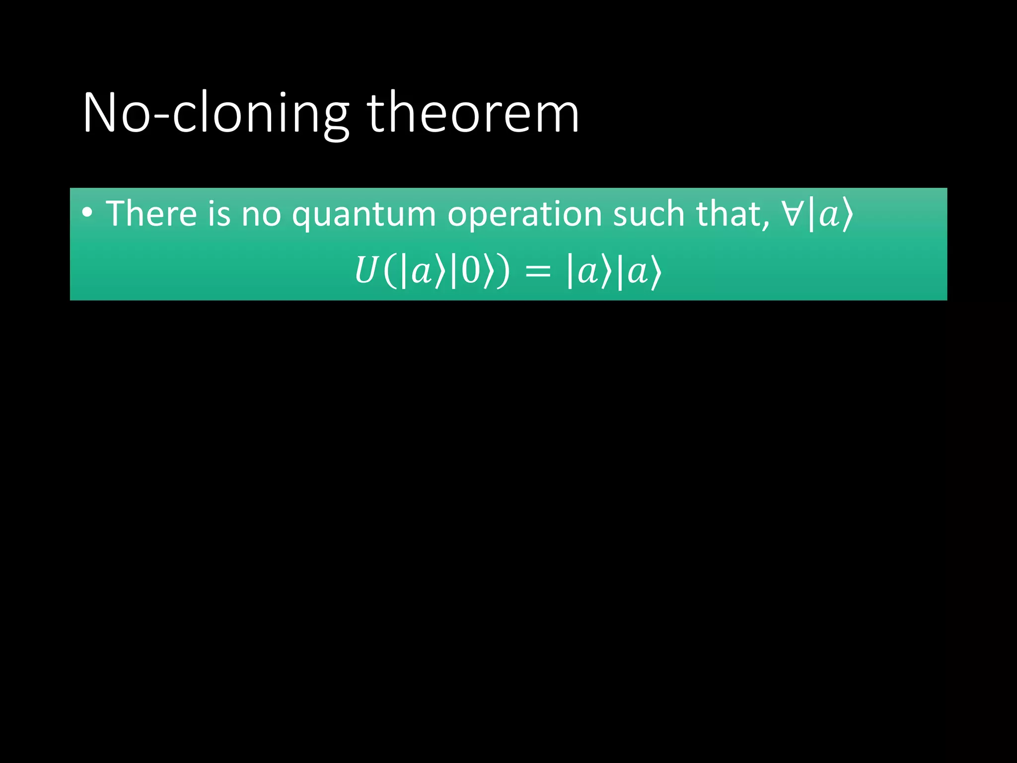
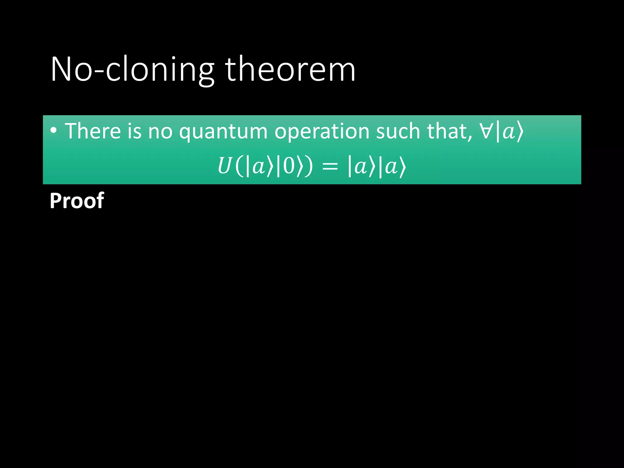
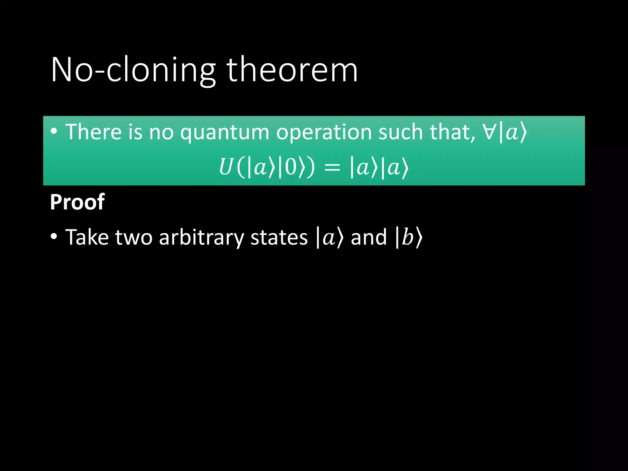
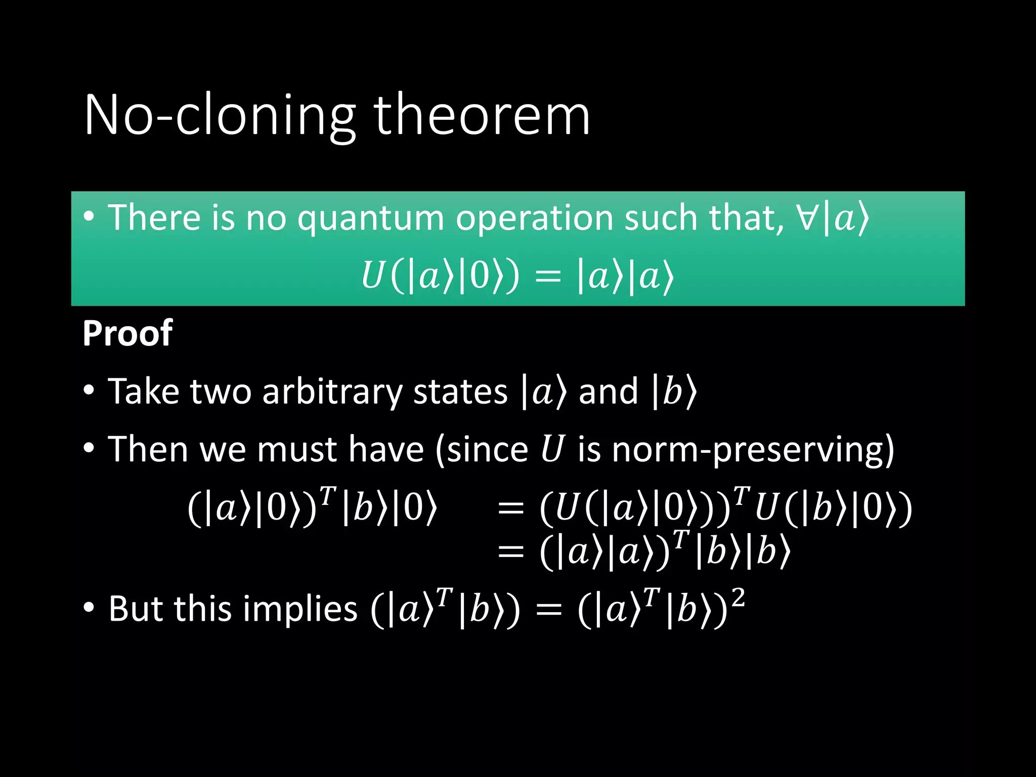
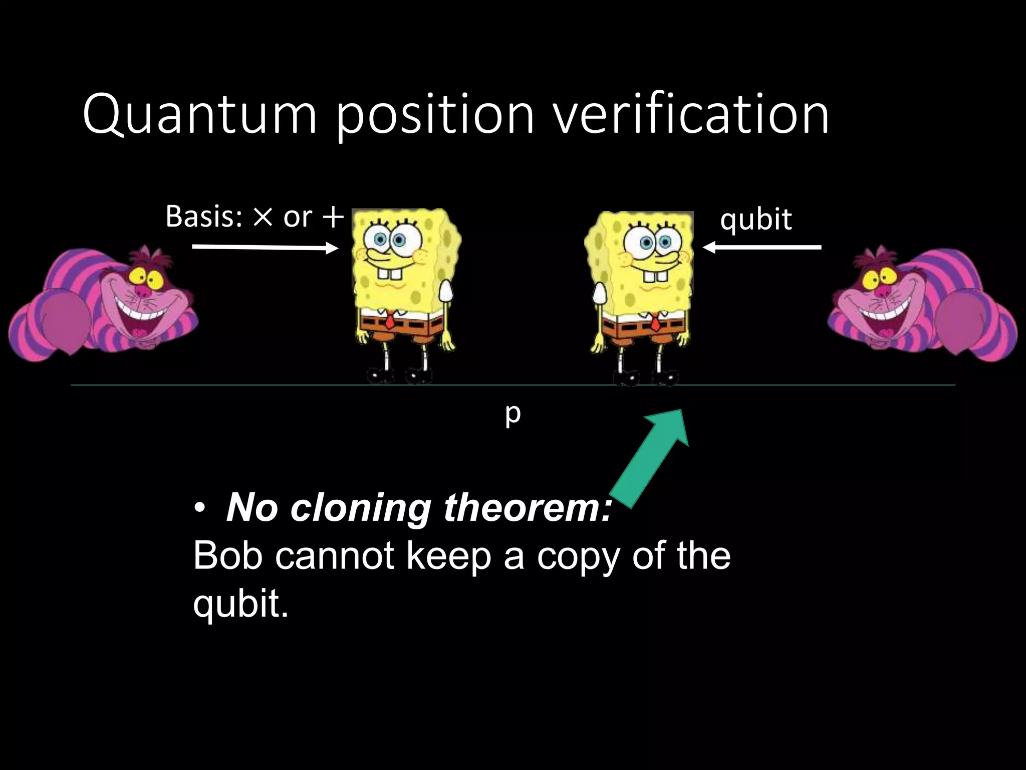
• No-cloning theorem: one cannot perfectly copy an
unknown quantum state.
• Information disturbance: if one does not know the
encoding basis, one cannot decode a qubit perfectly
without perturbing (collapsing) it.](https://image.slidesharecdn.com/giannicolascarpa-slides-190417135656/75/A-short-introduction-to-Quantum-Computing-and-Quantum-Cryptography-113-2048.jpg)


![But wait!!!
p
Open problem: actually prove
the security of this protocol!
[Buhrman et al, 2011]](https://image.slidesharecdn.com/giannicolascarpa-slides-190417135656/75/A-short-introduction-to-Quantum-Computing-and-Quantum-Cryptography-160-2048.jpg)

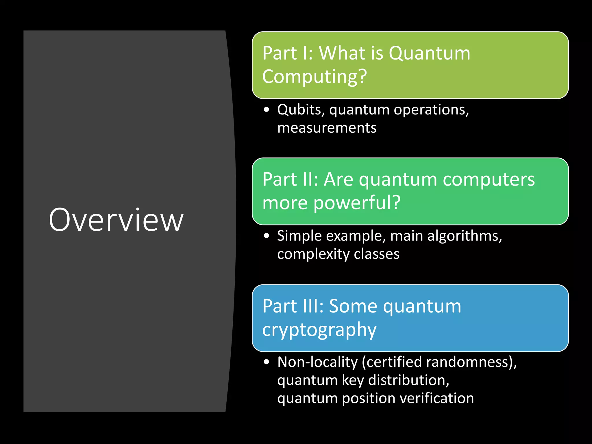
The document provides an introduction to quantum computing, covering essential concepts such as qubits, operations, and measurements. It compares the power of quantum computers to classical ones, exemplified through parity computation and highlights quantum parallelism, where quantum computers can execute multiple calculations simultaneously. Key topics include quantum cryptography and algorithms, emphasizing the unique features of quantum mechanics like superposition and entanglement.
Introduces quantum computing and its overview, covering qubits, algorithms, and cryptography.
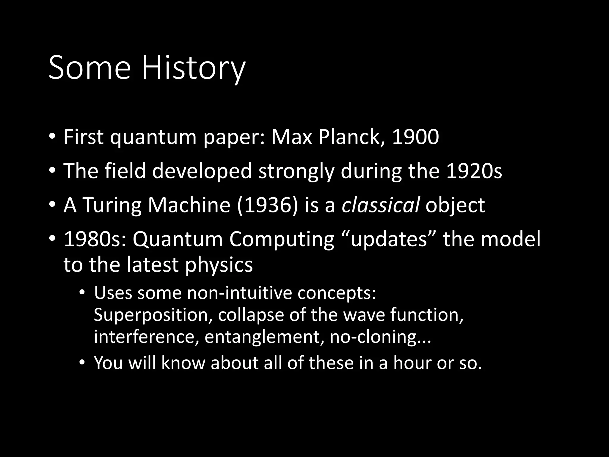
Explains quantum computation using Schrödinger's cat as an analogy, and discusses historical context.
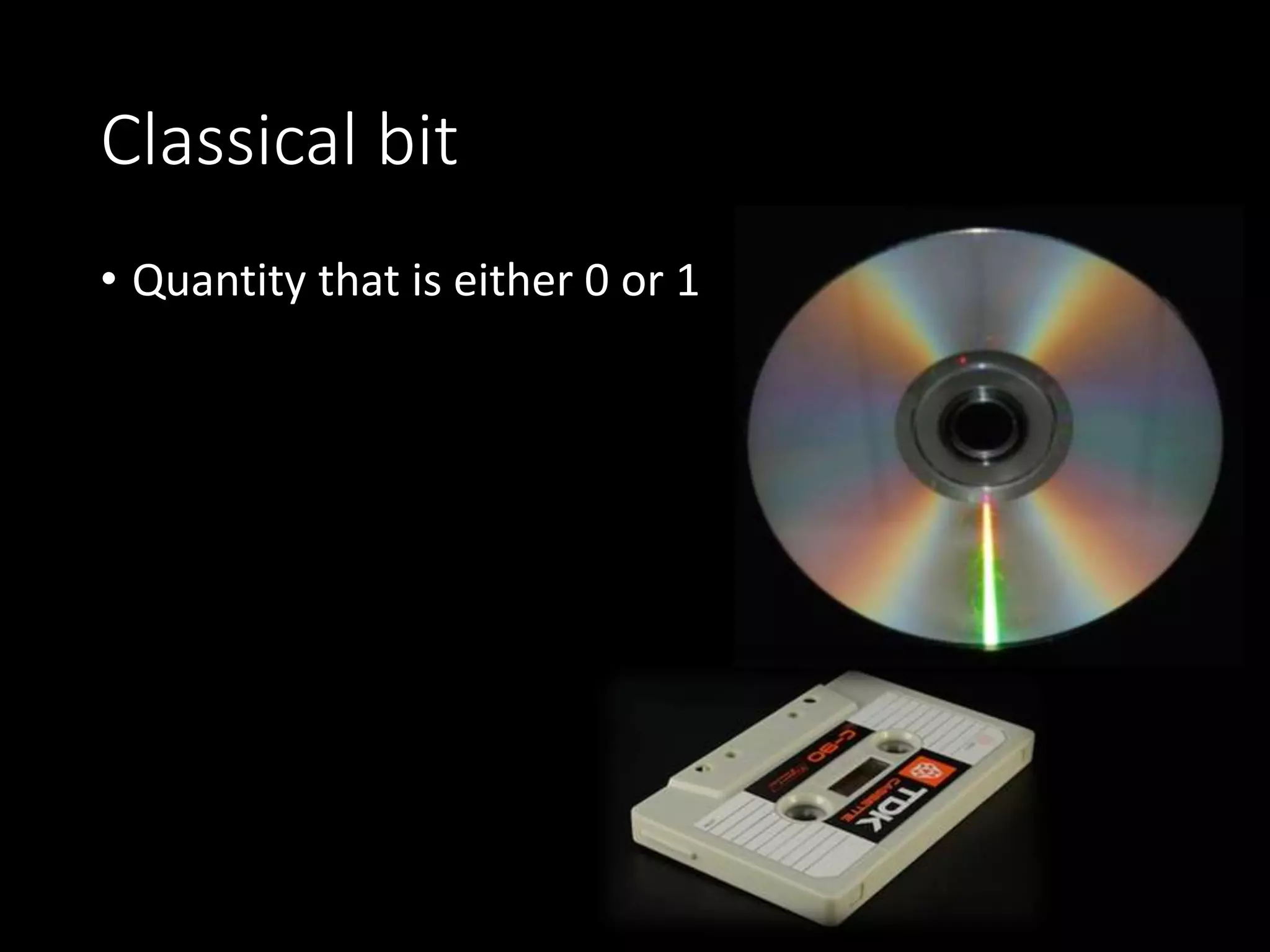
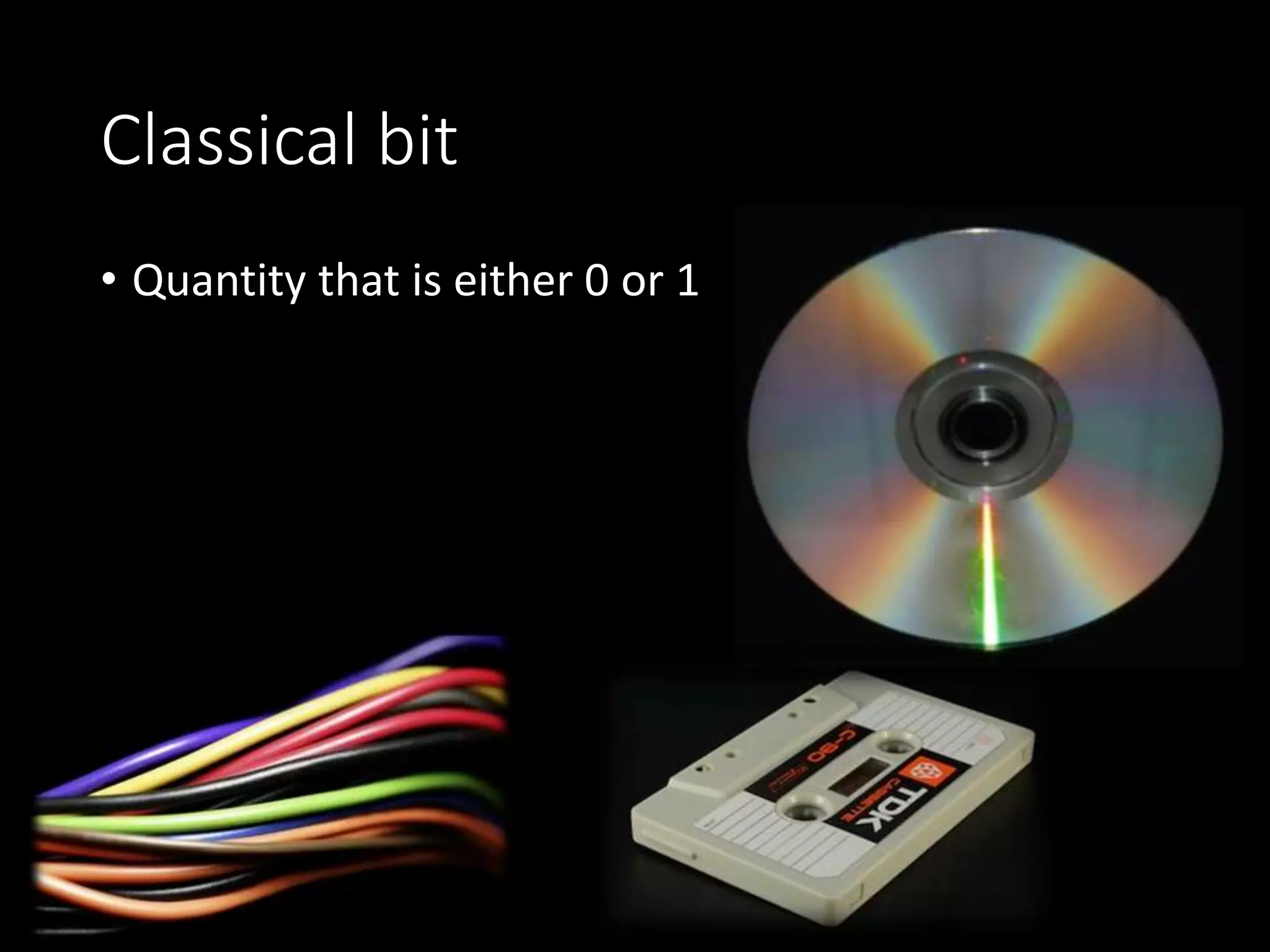
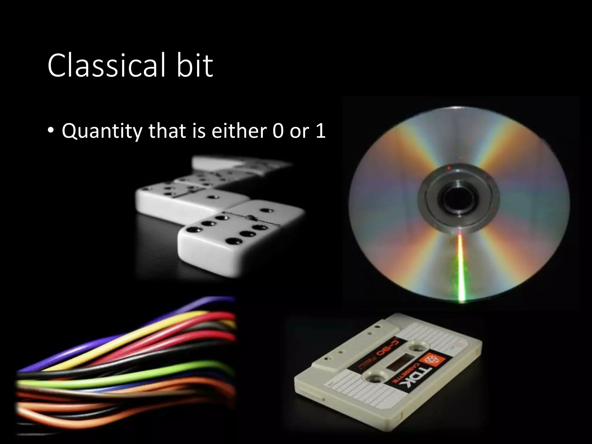
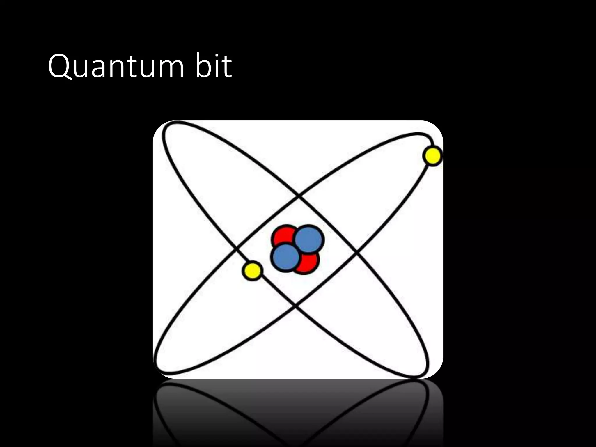
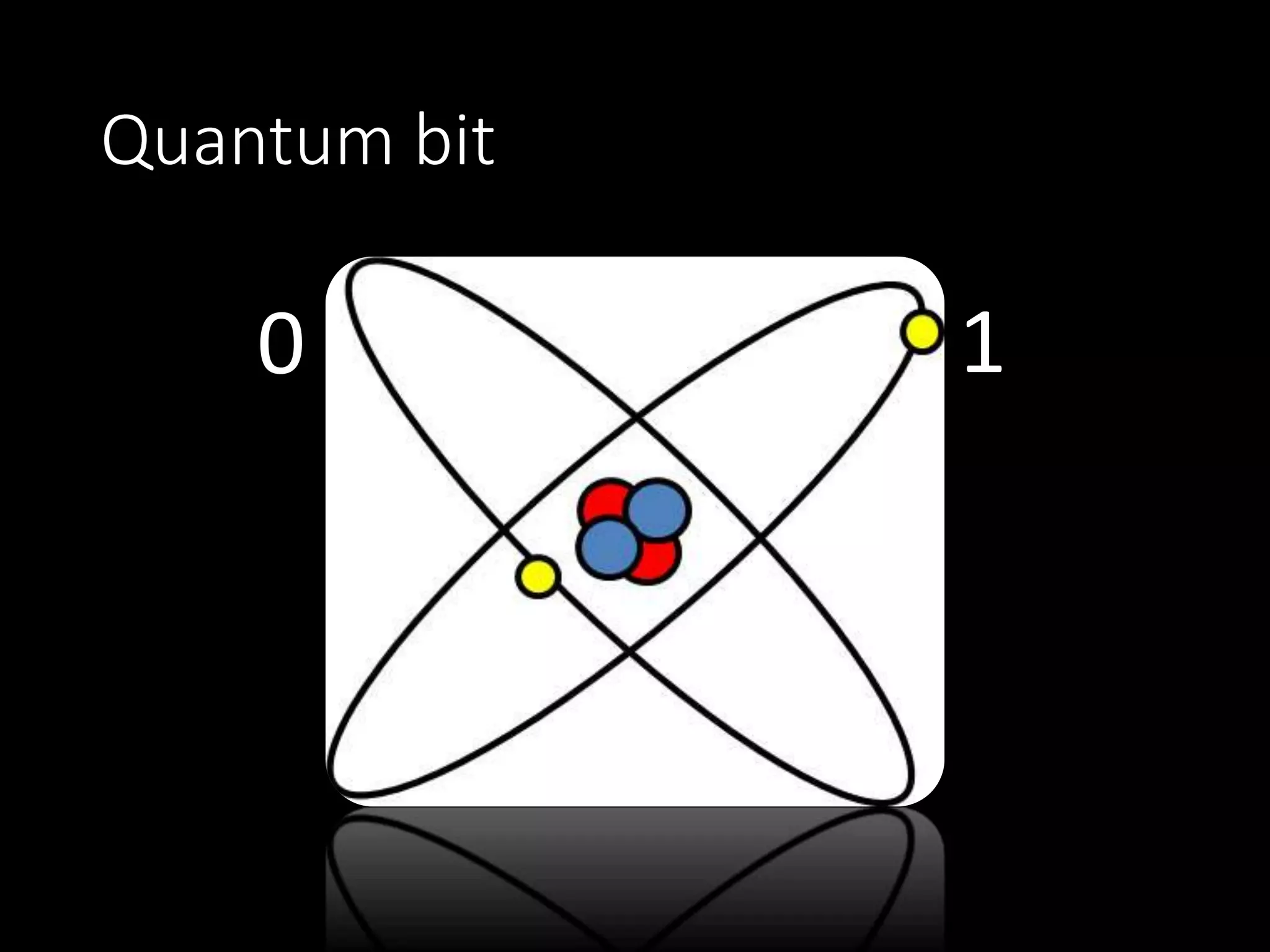
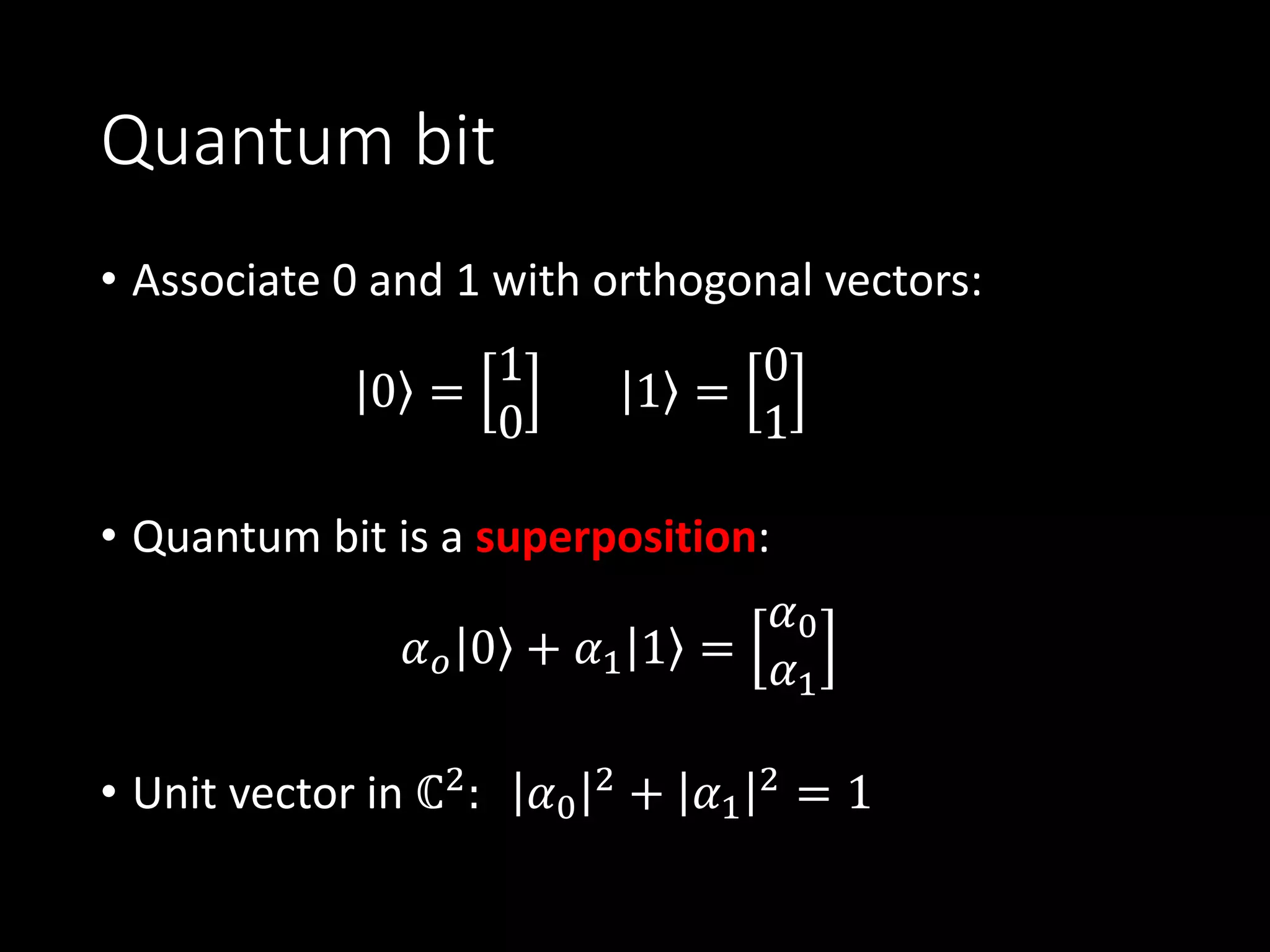
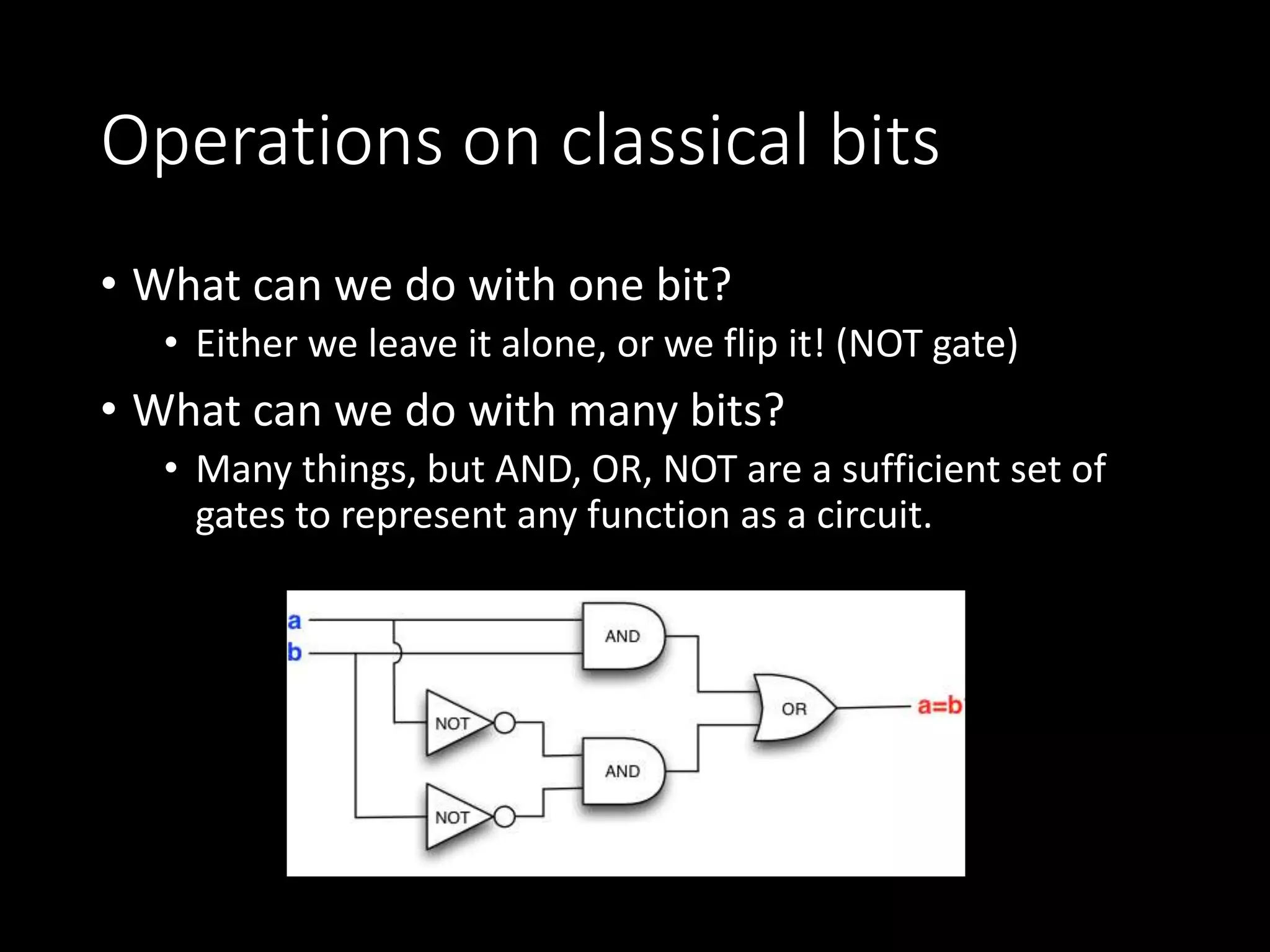
Details on classical bits, their binary nature, and introduces quantum bits (qubits) associated with superposition.
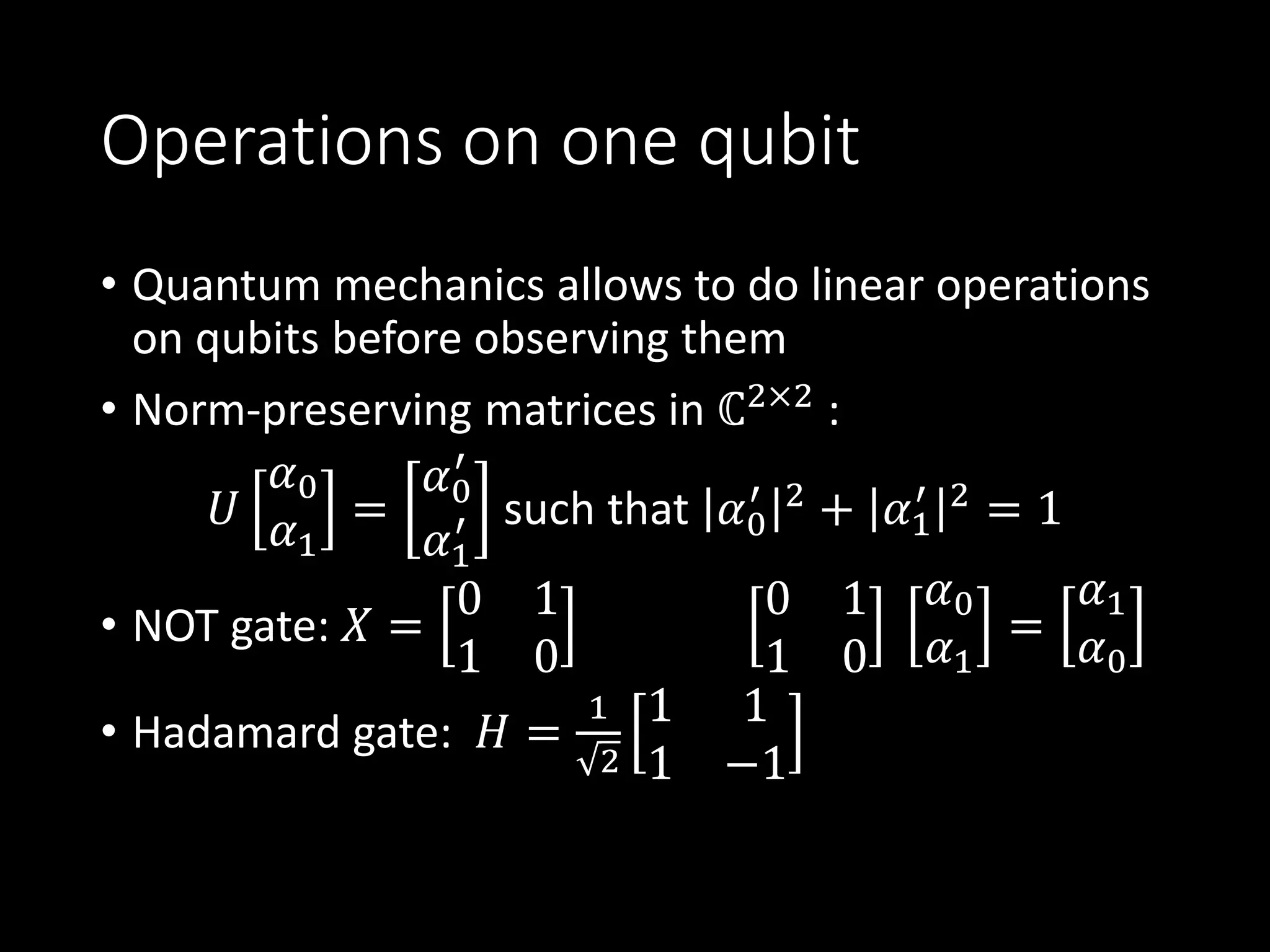
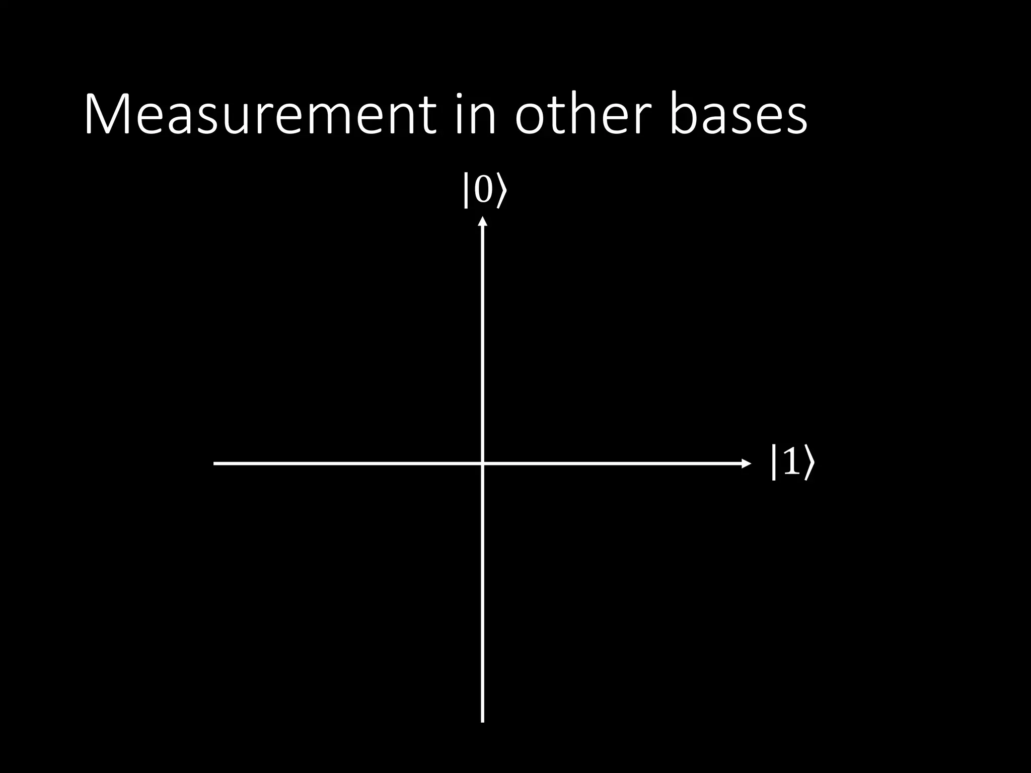
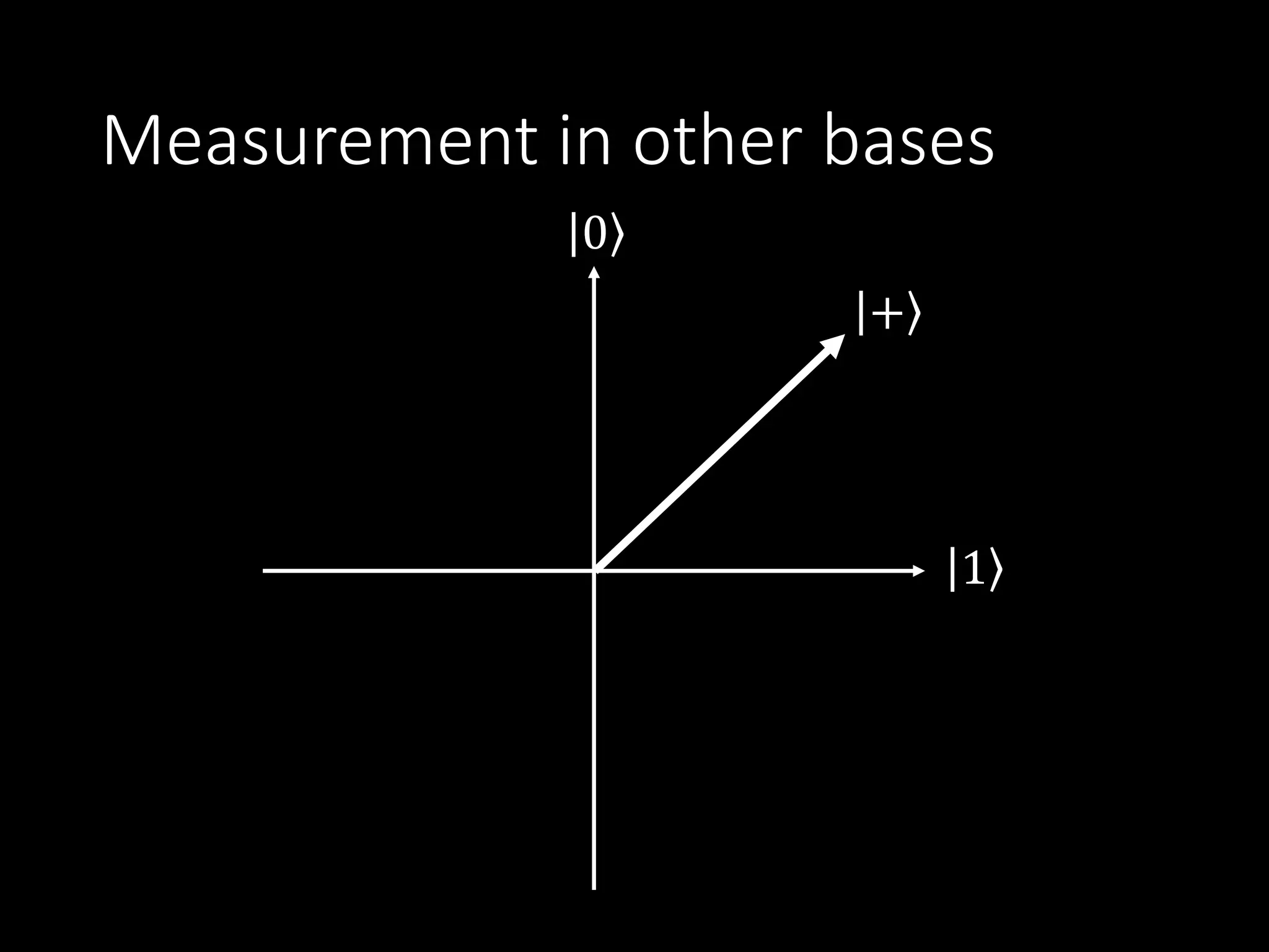
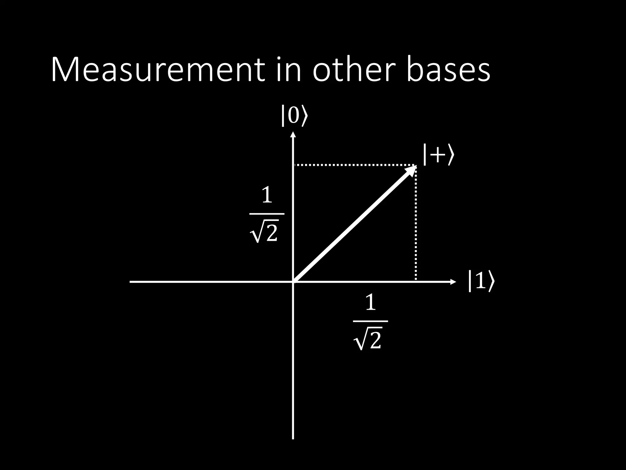
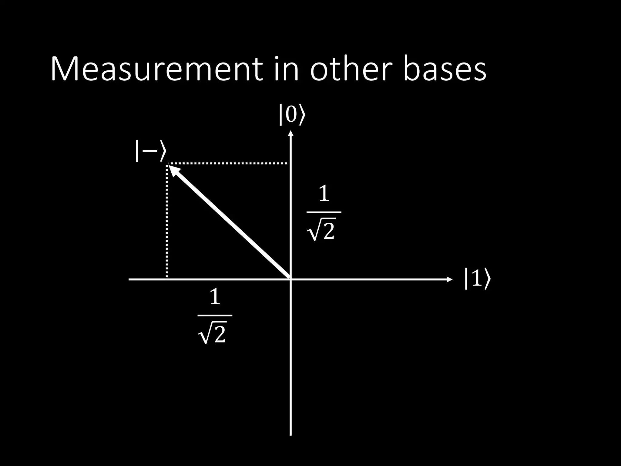
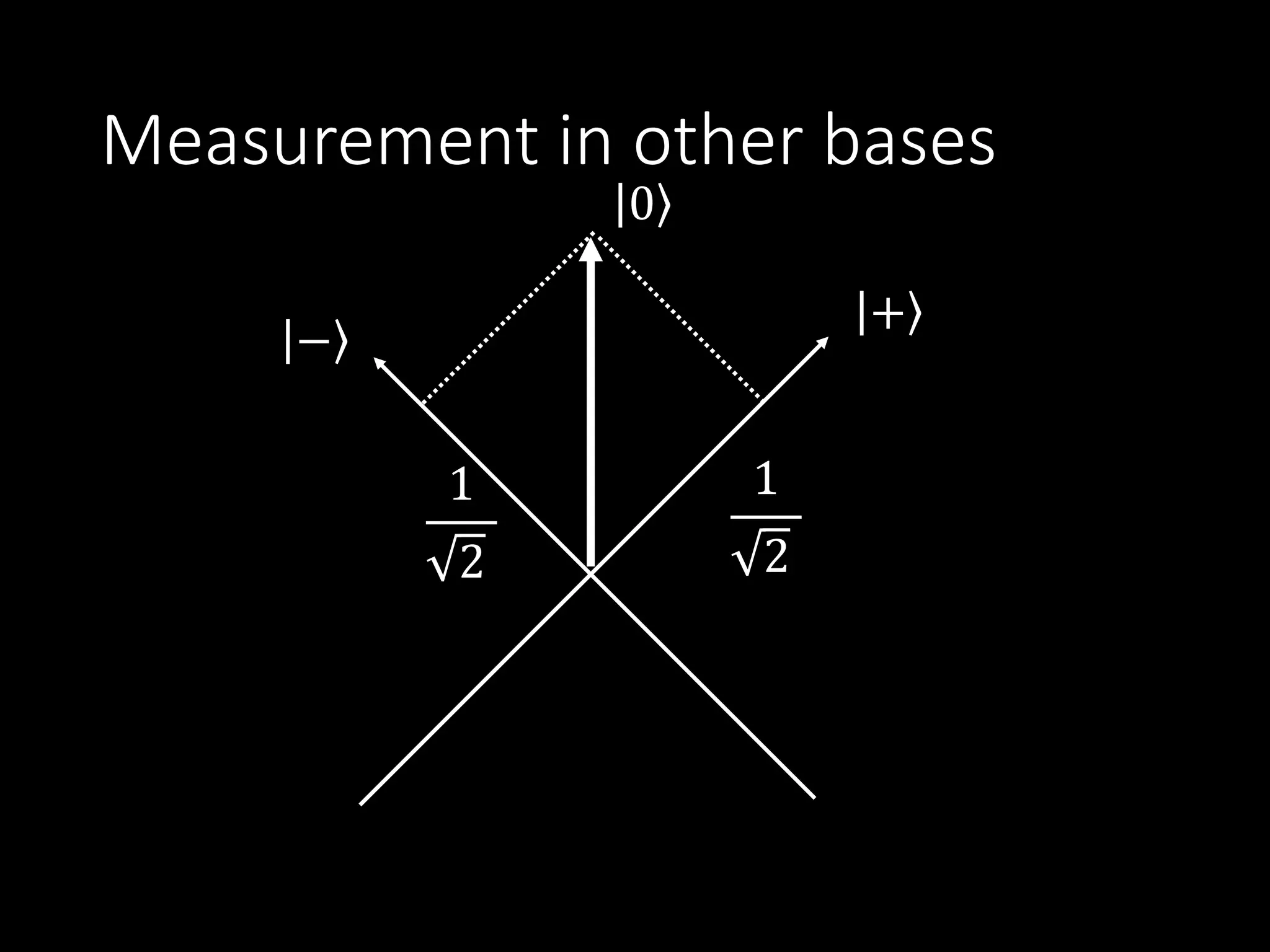
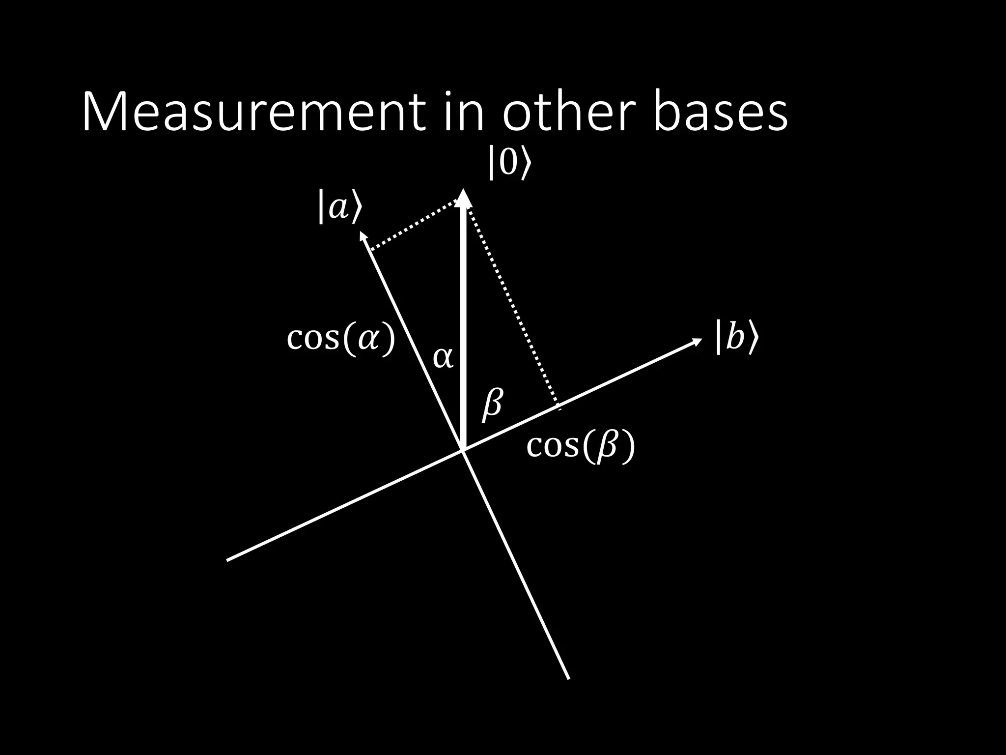
Discusses the process of measurement in quantum computing and the operations that can be performed on qubits.
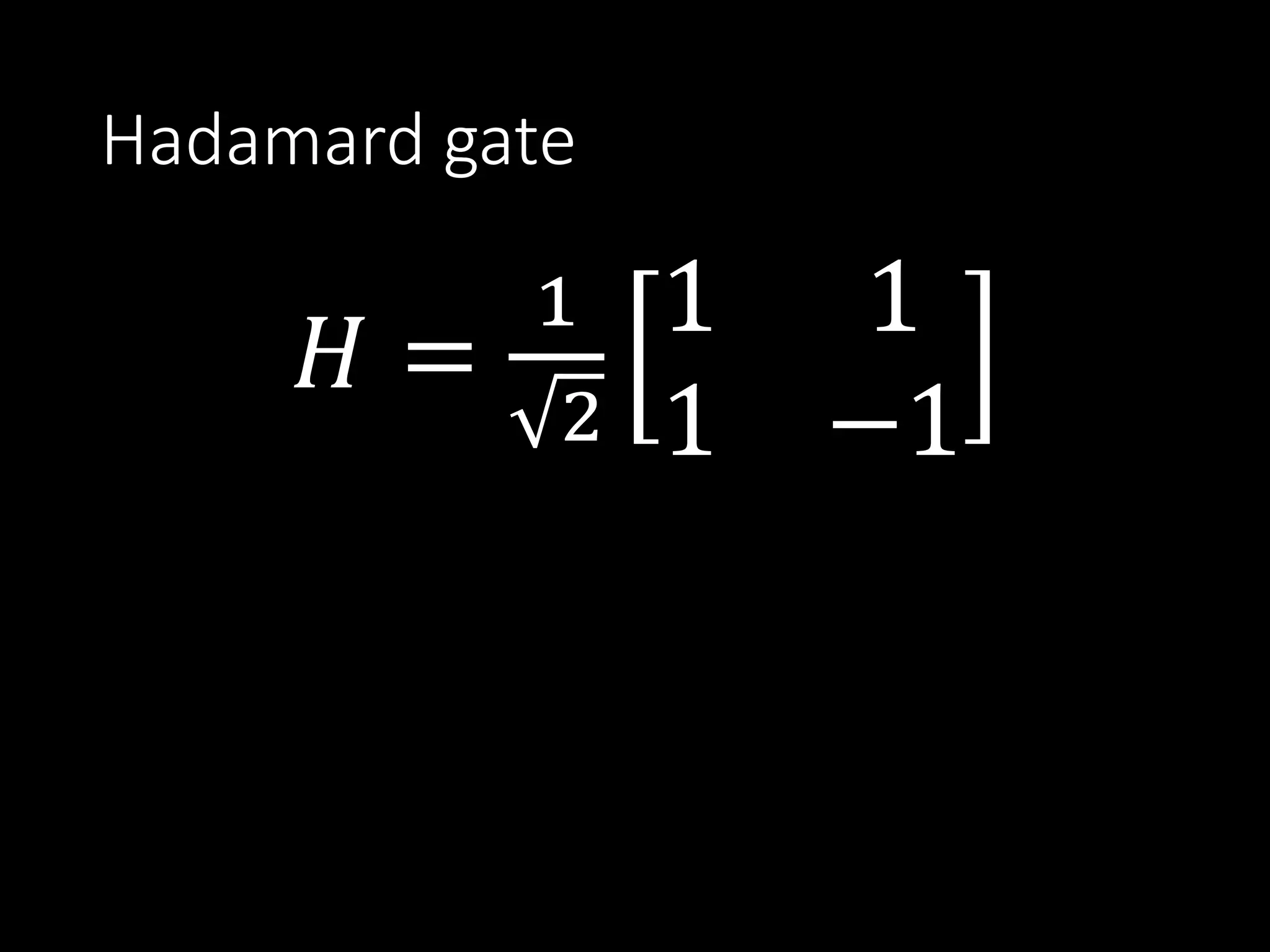
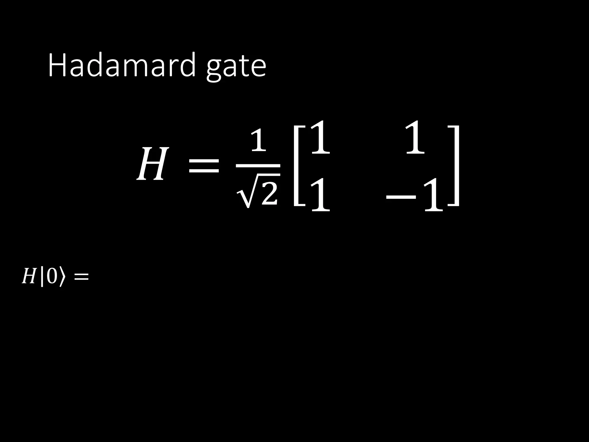
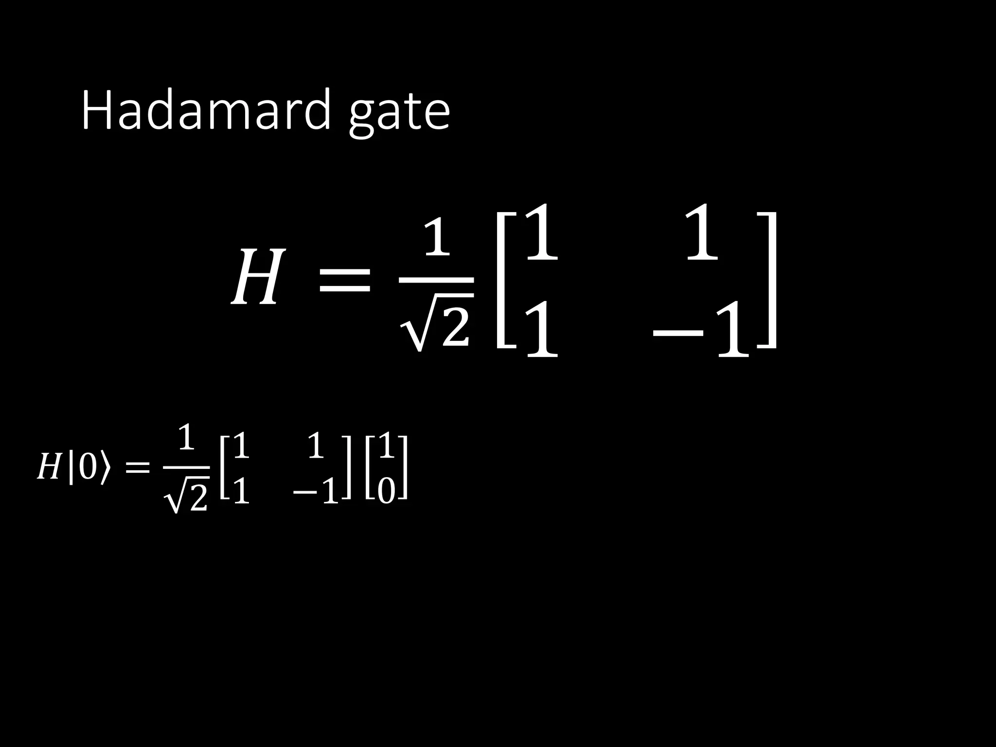
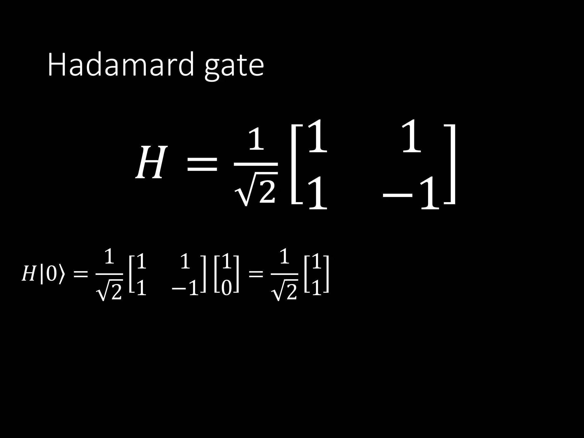
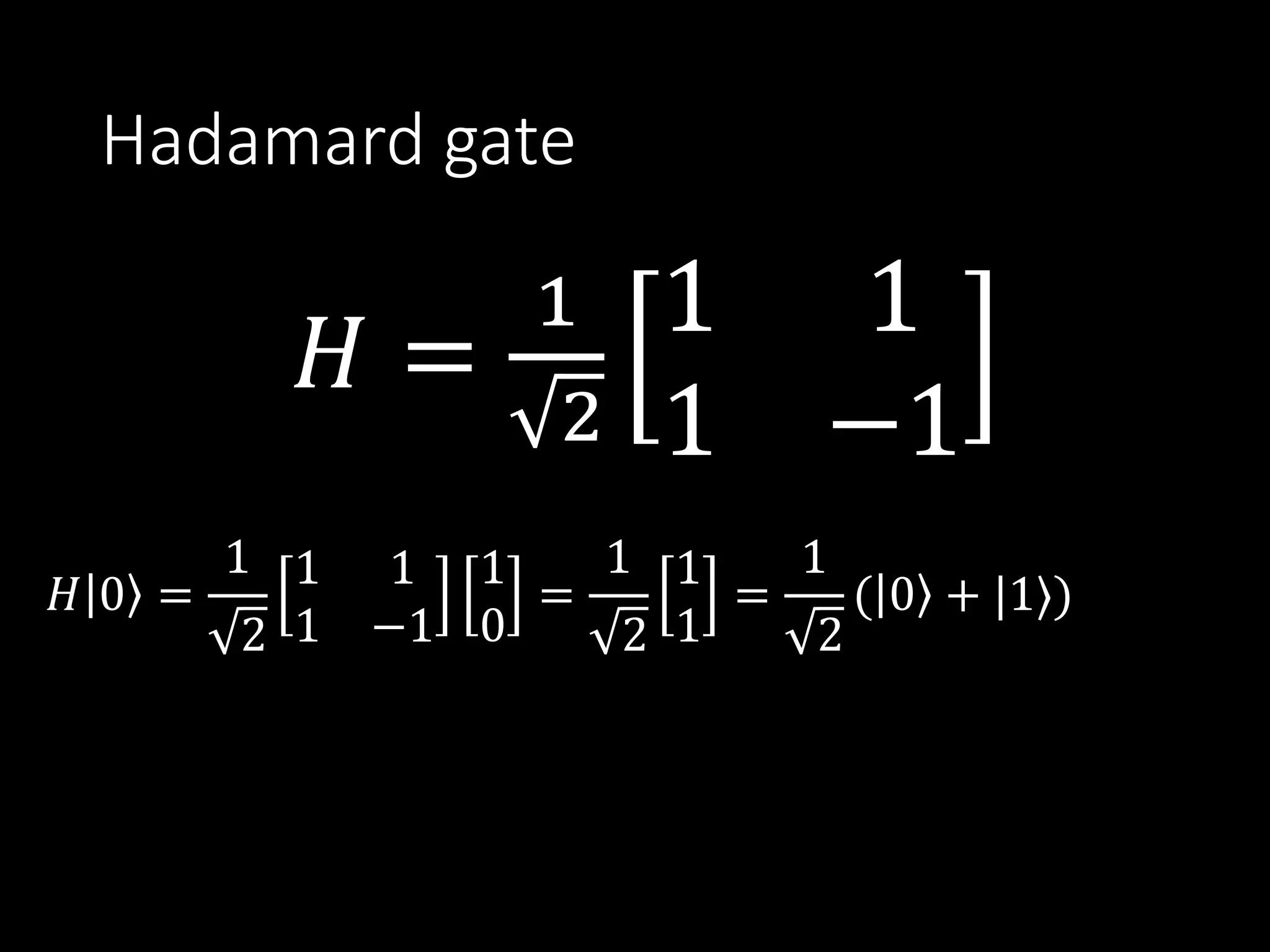
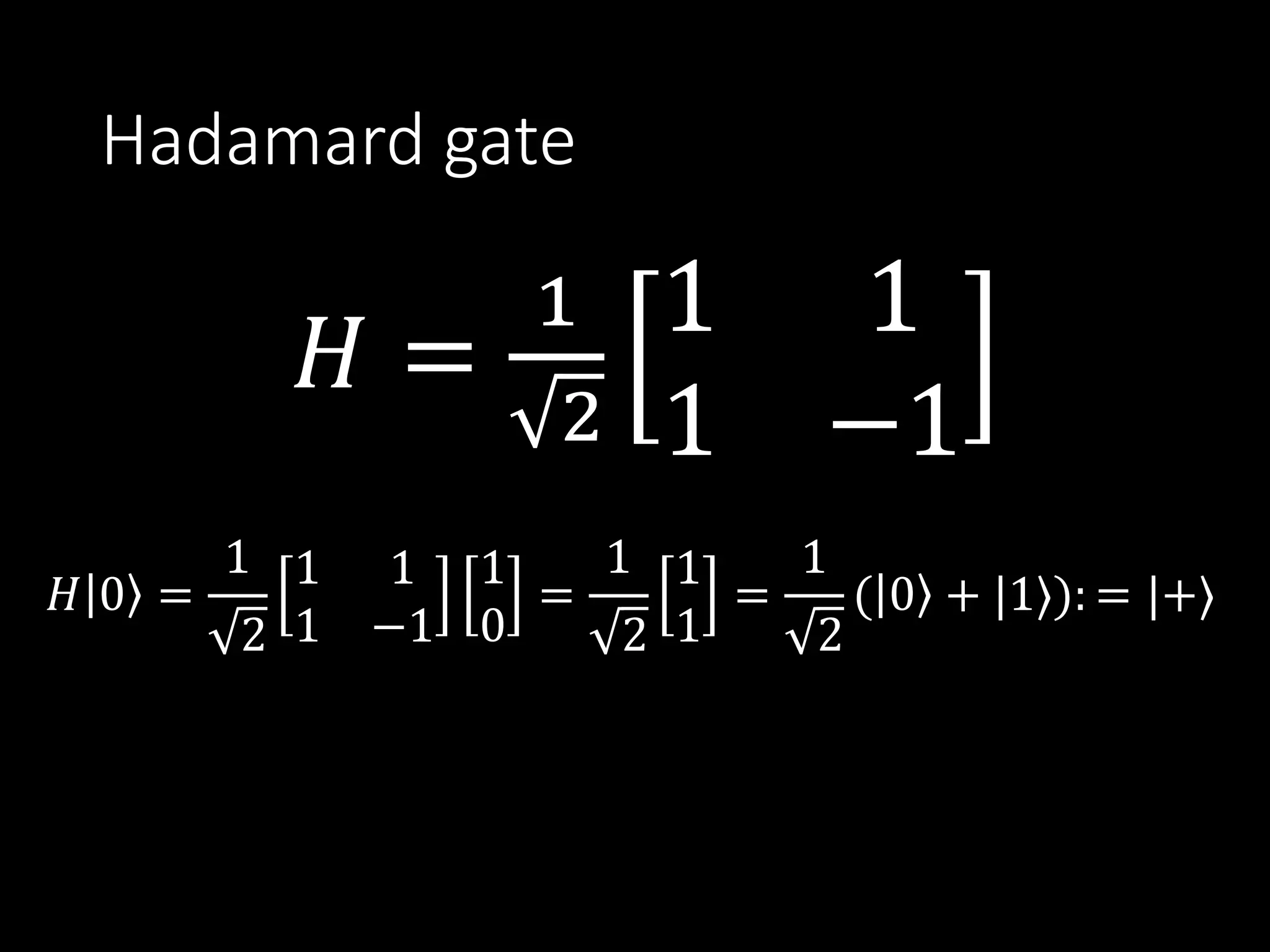
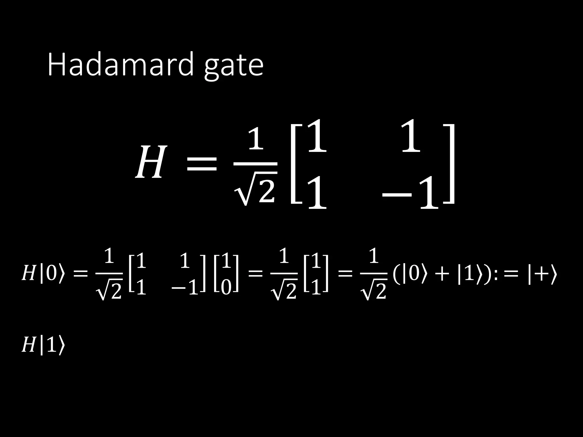
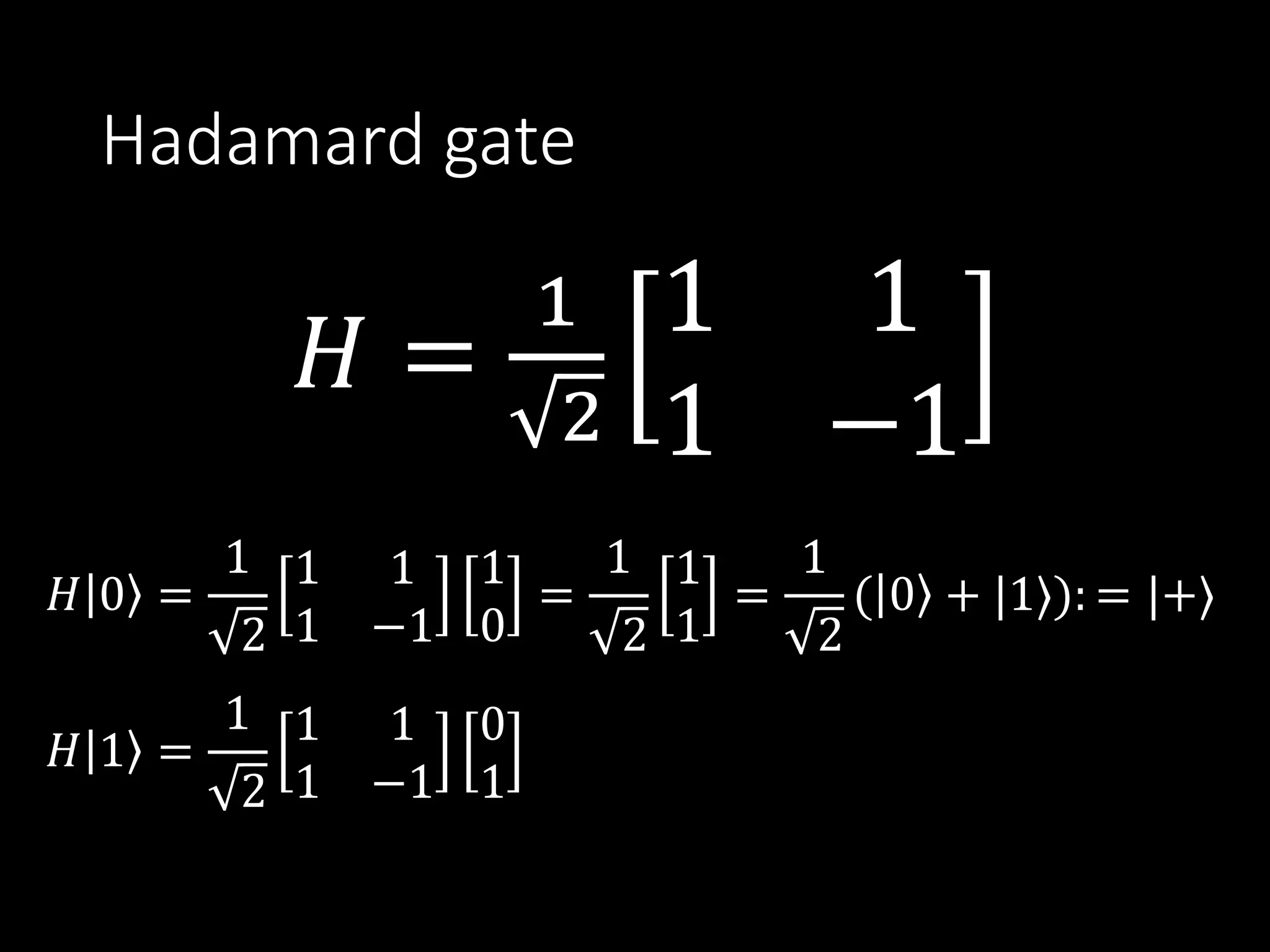
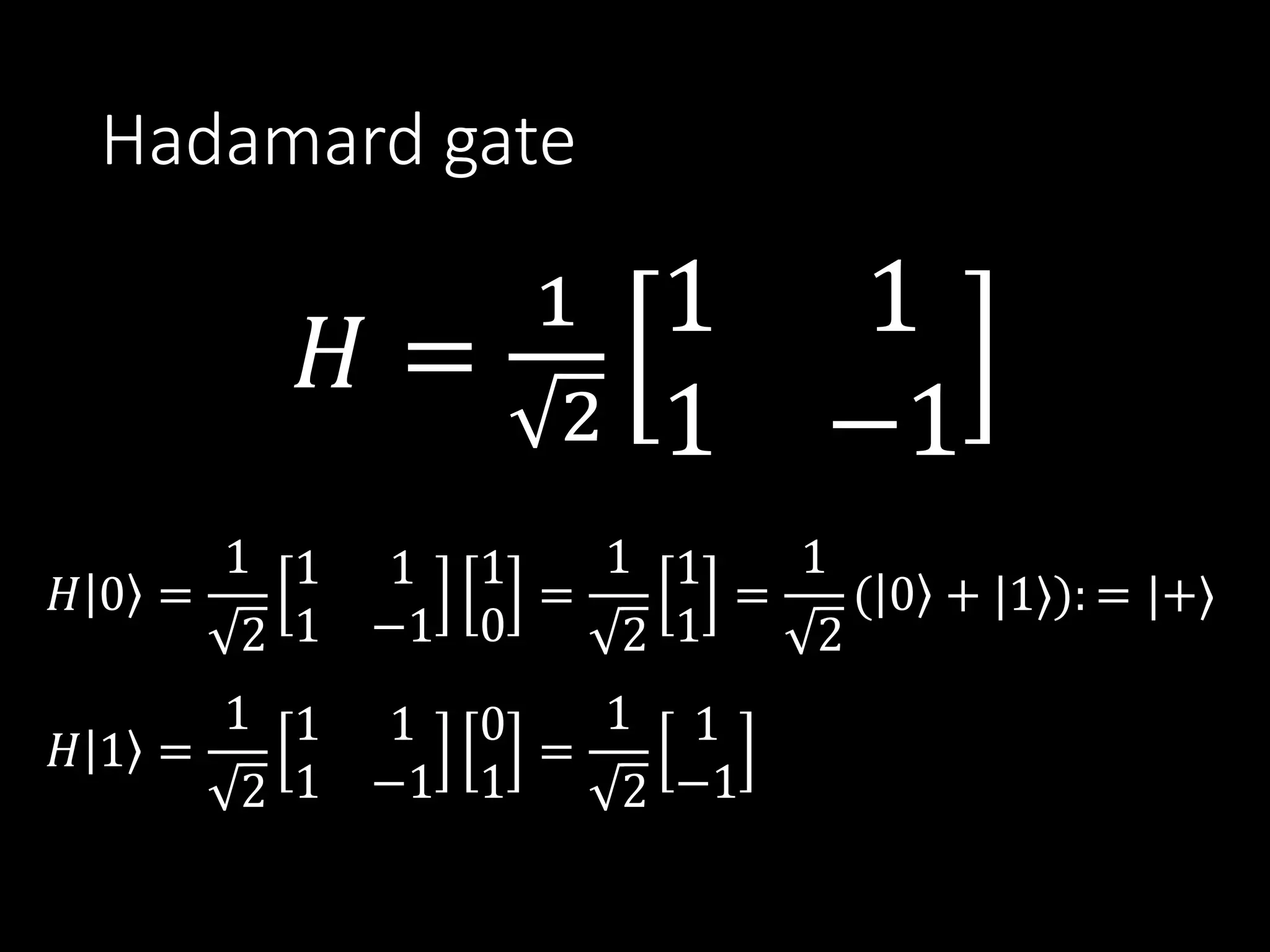
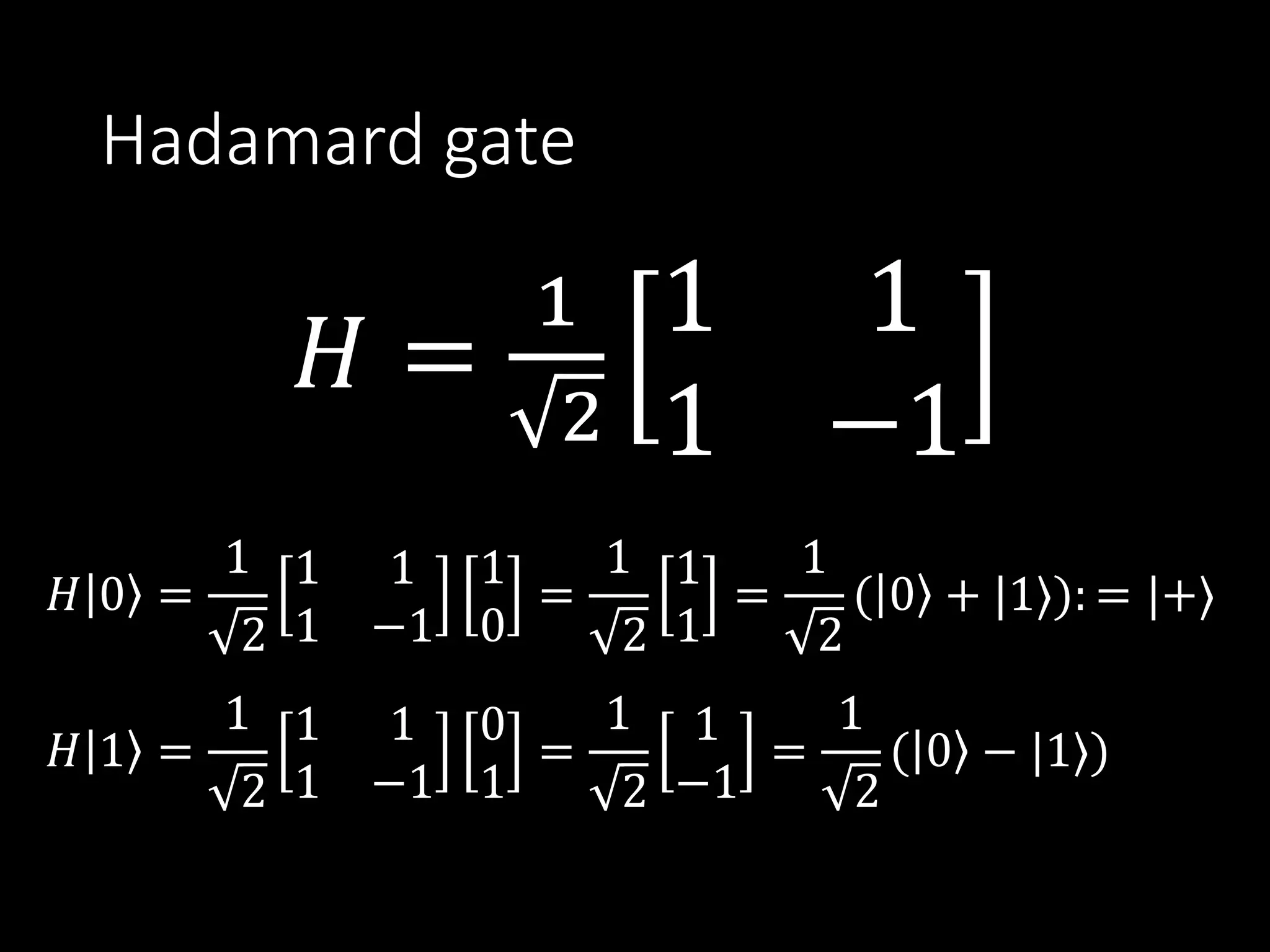
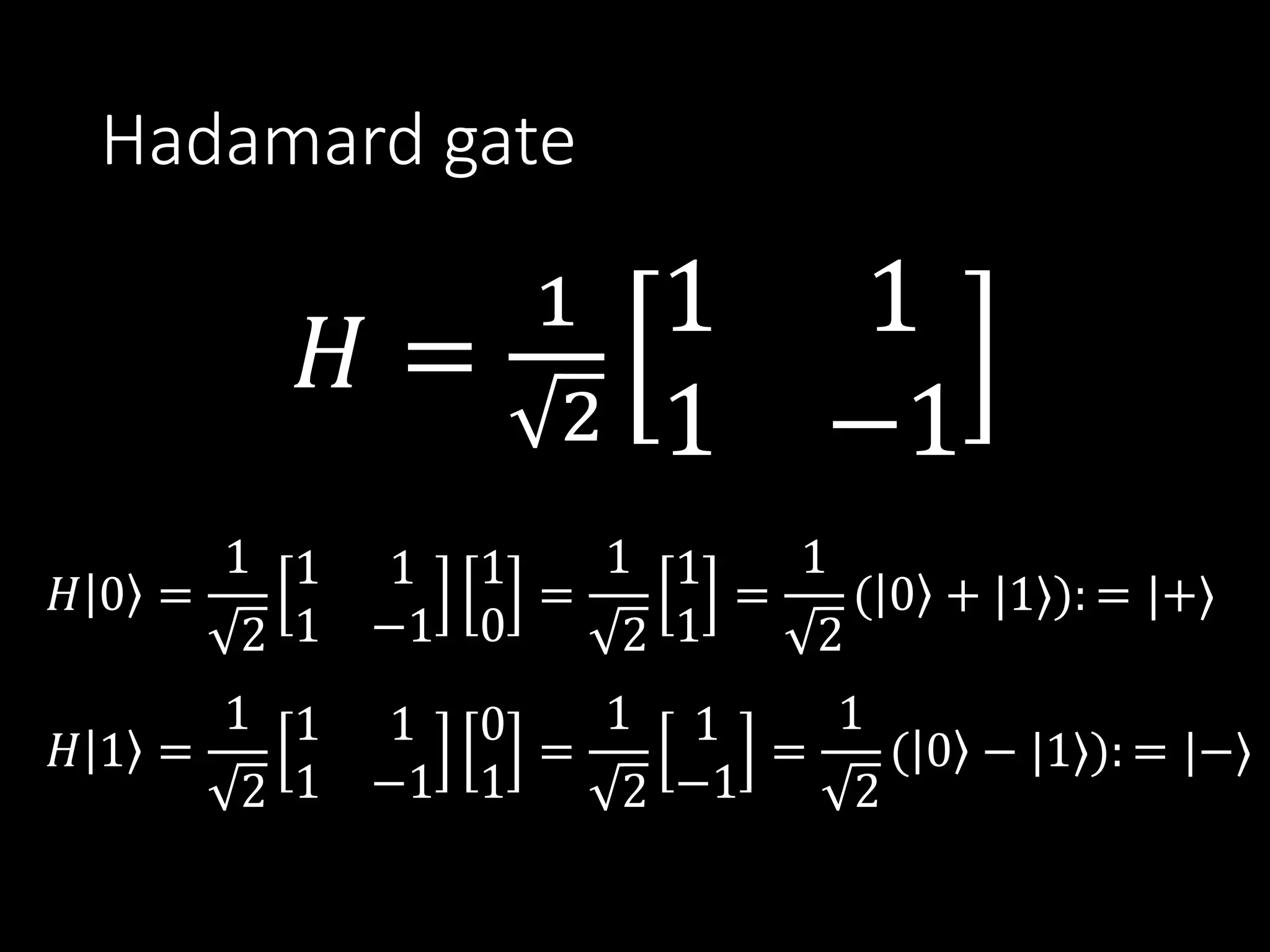
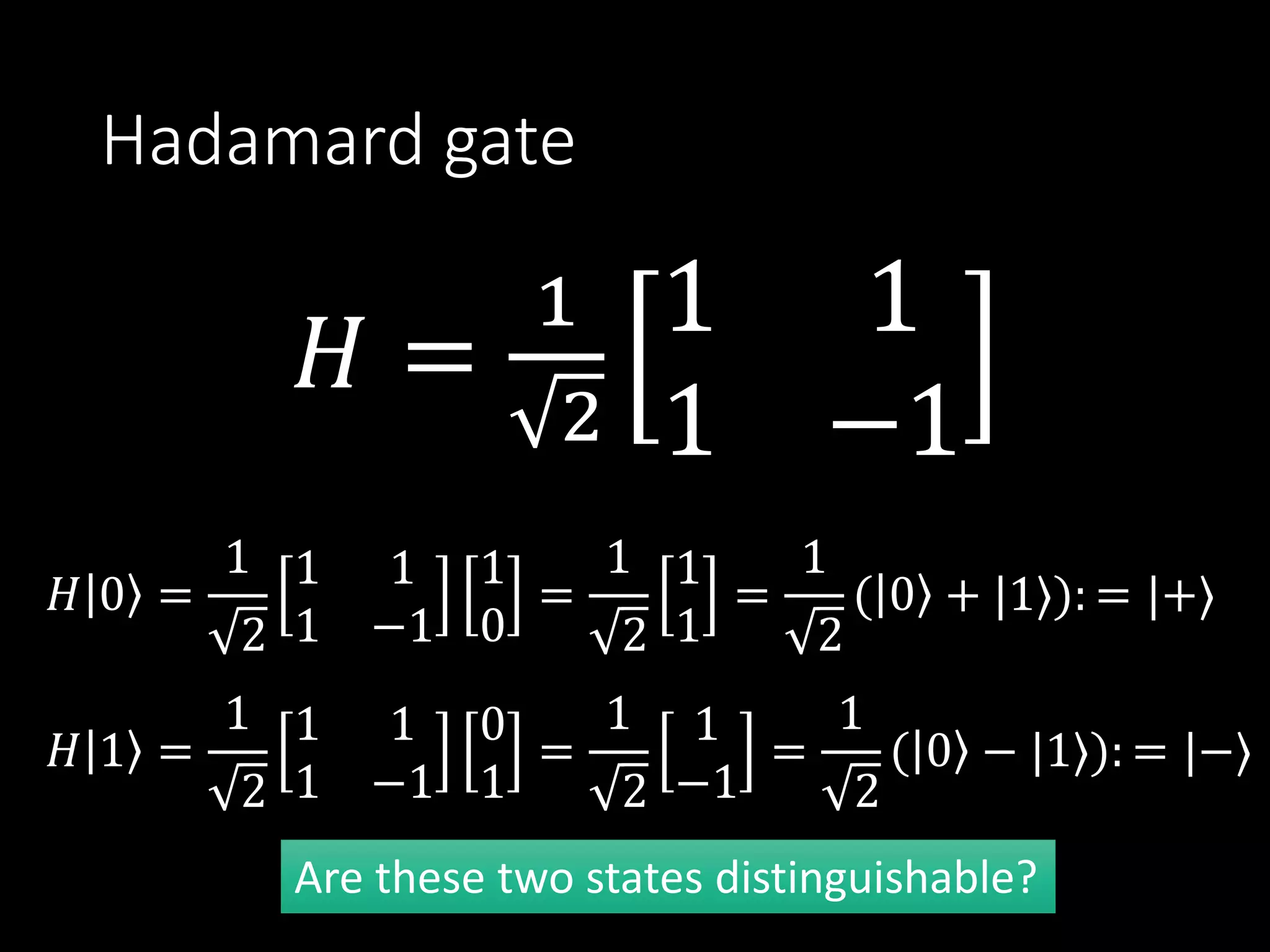
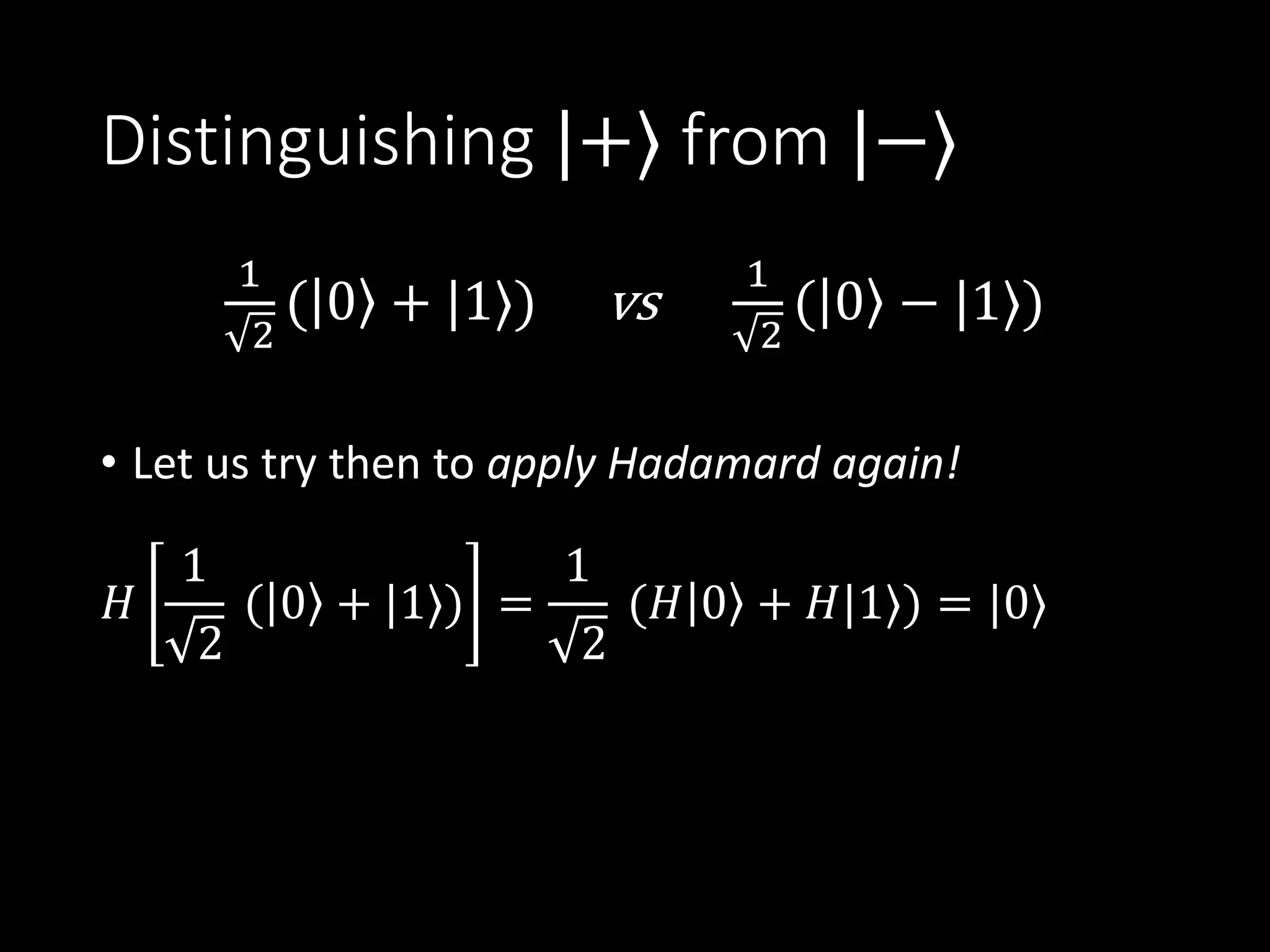
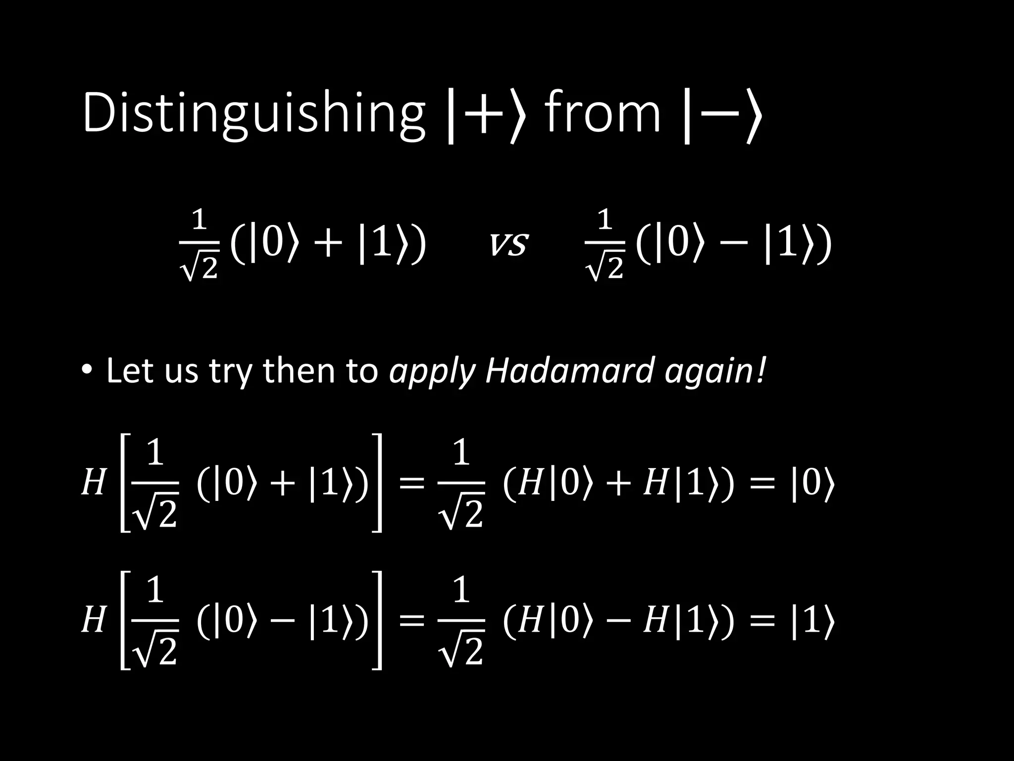
In-depth explanation of the Hadamard gate, its matrix representation, and its effects on qubits.
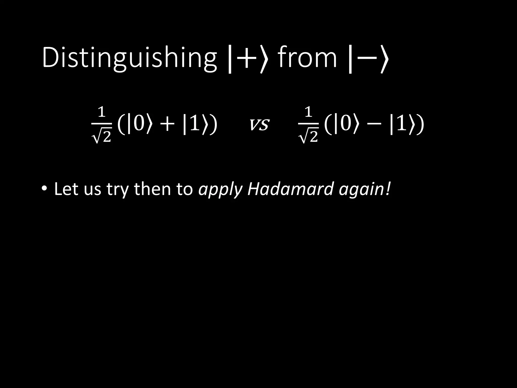
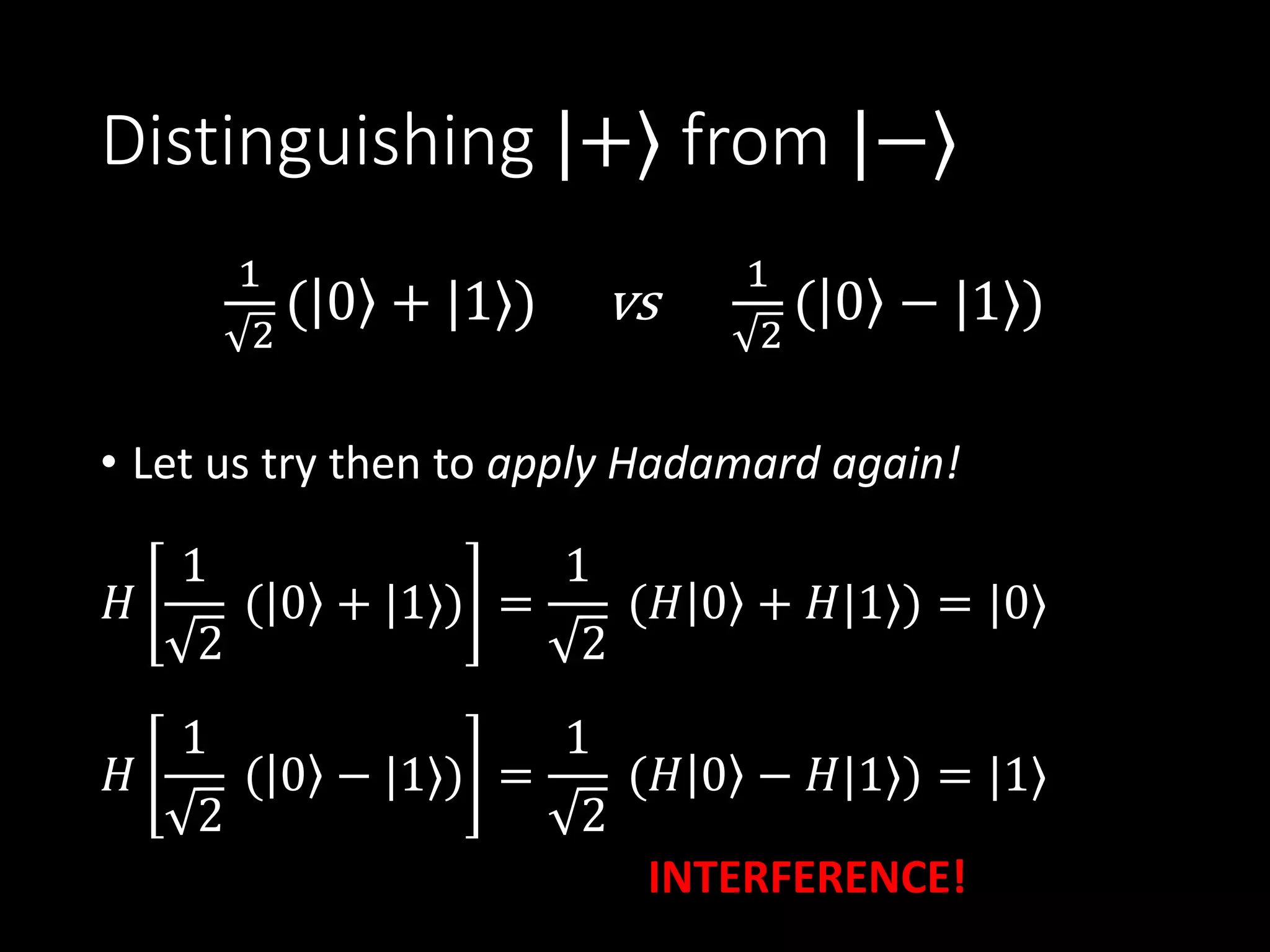
Describes how to distinguish between quantum states, particularly using the Hadamard gate and interference.
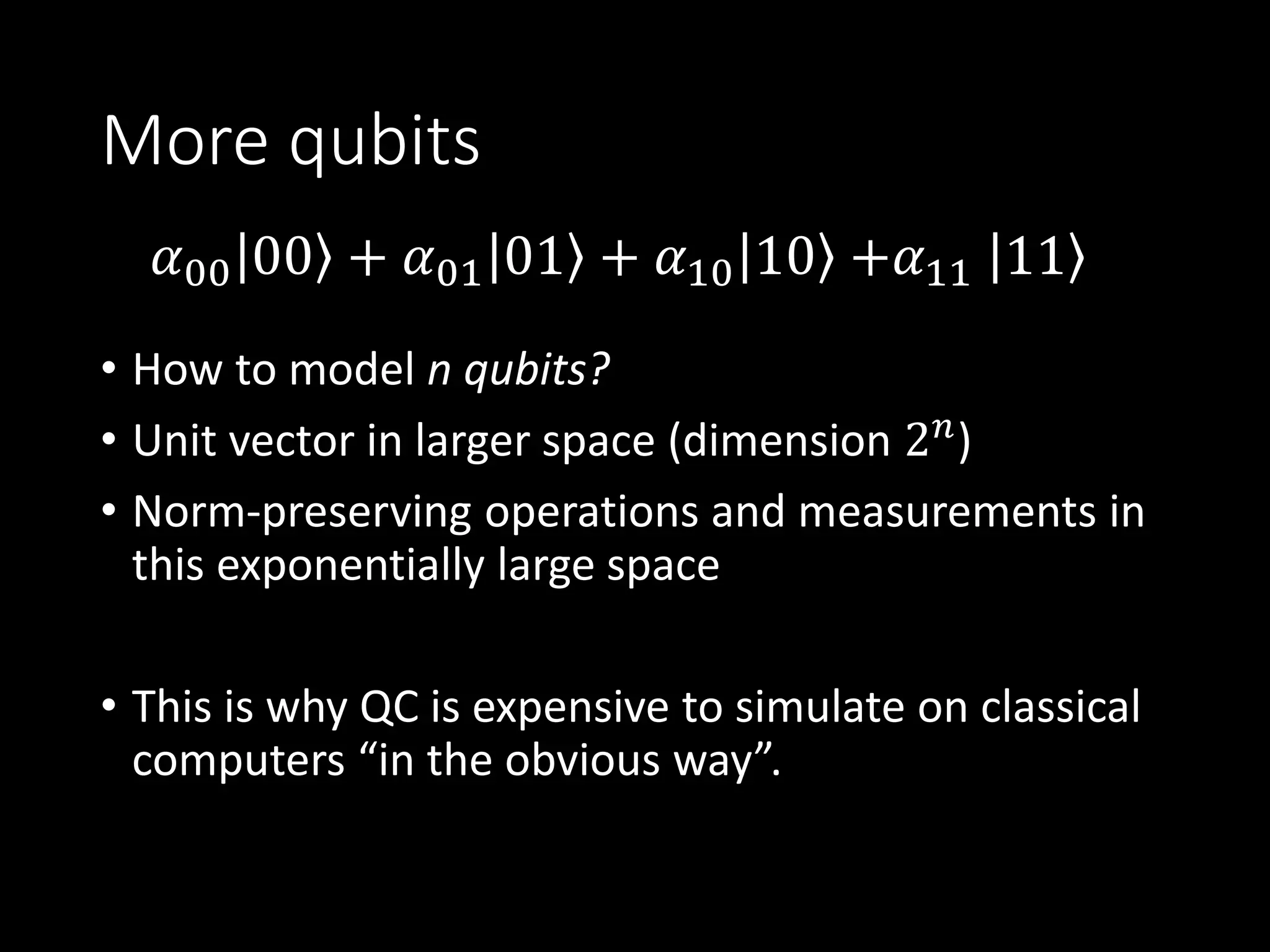
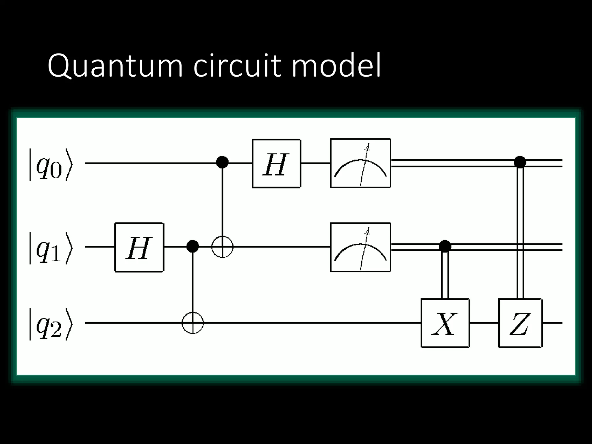
Explains modeling multiple qubits and presents the quantum circuit model.
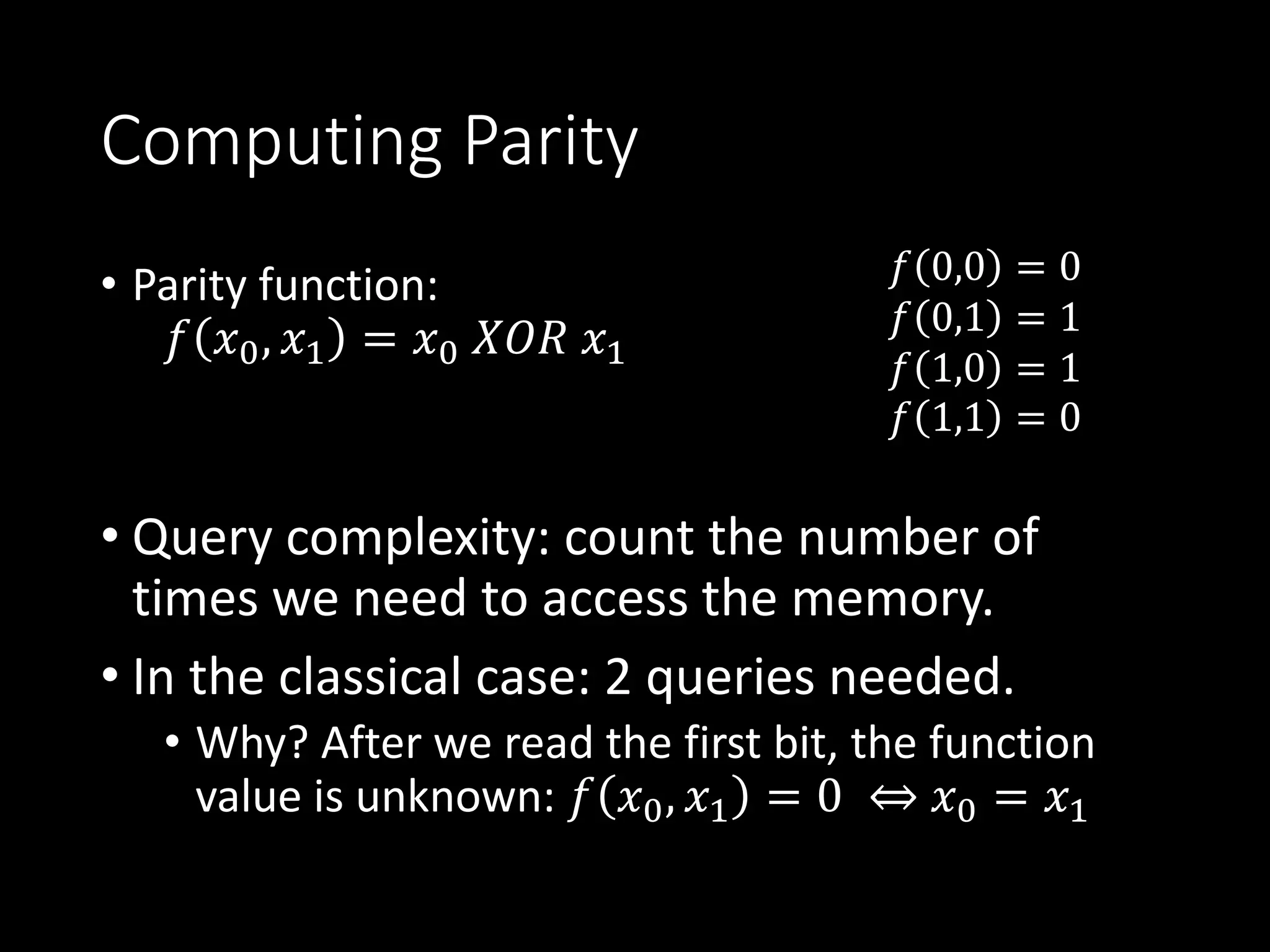
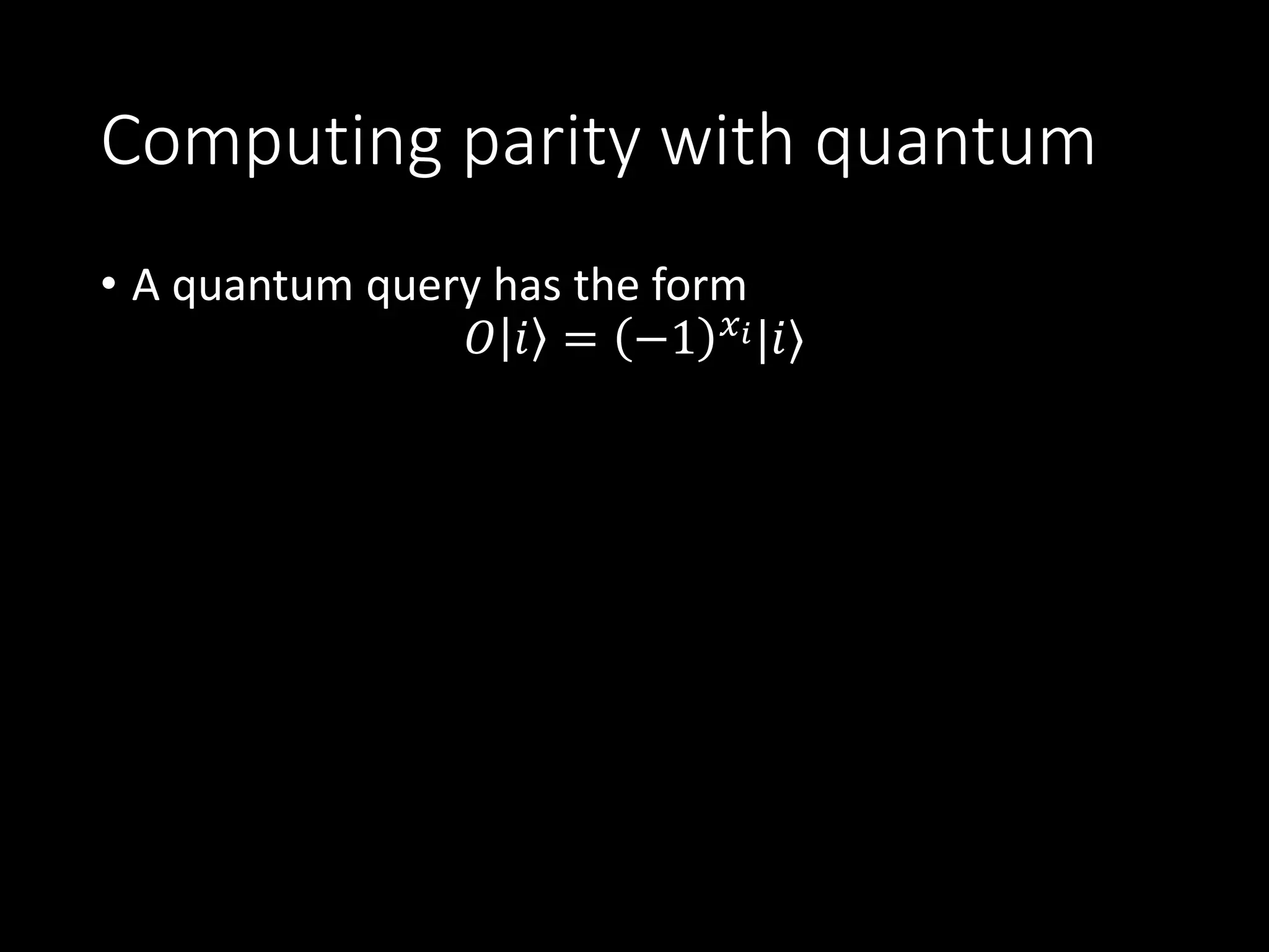
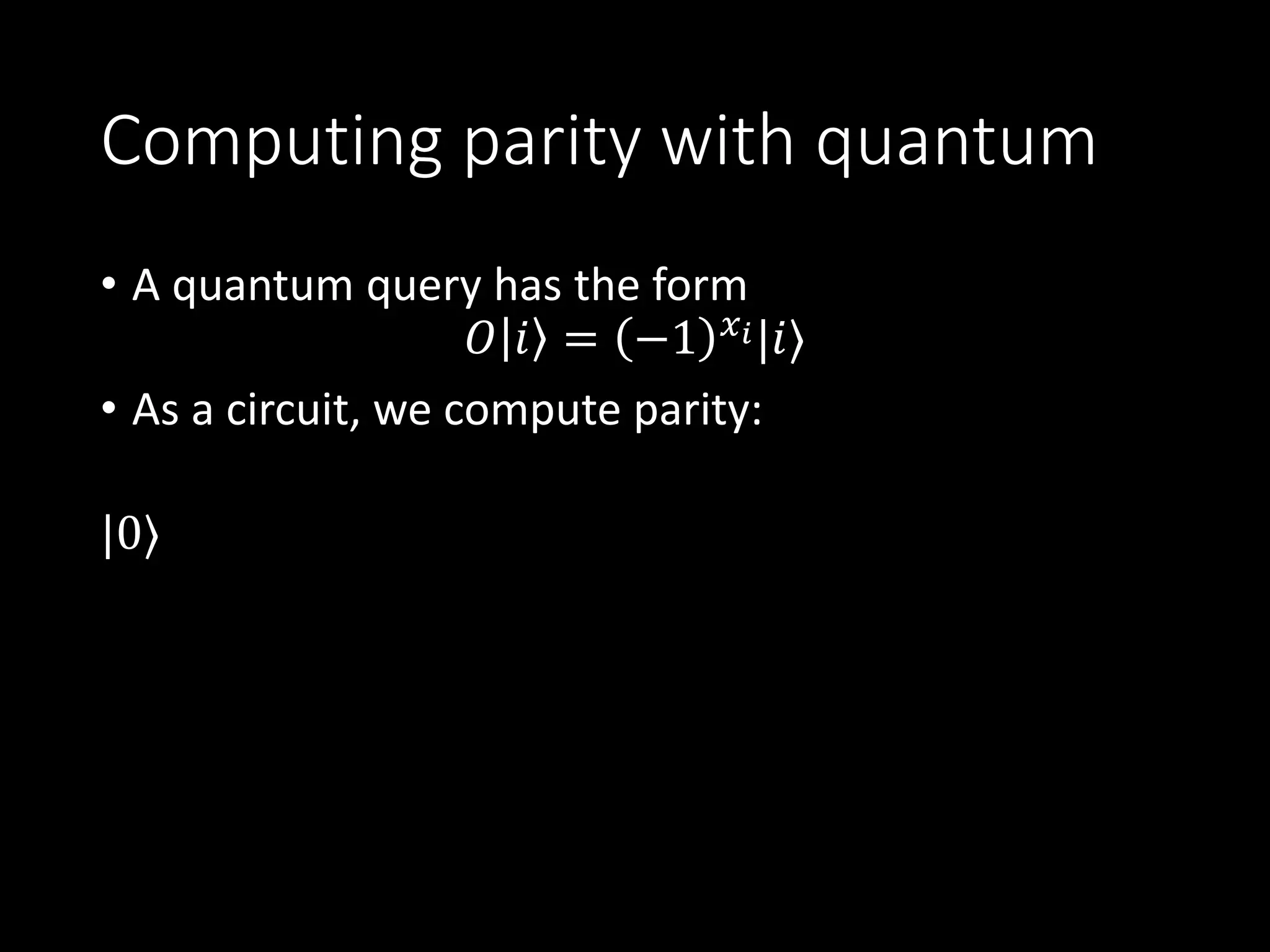
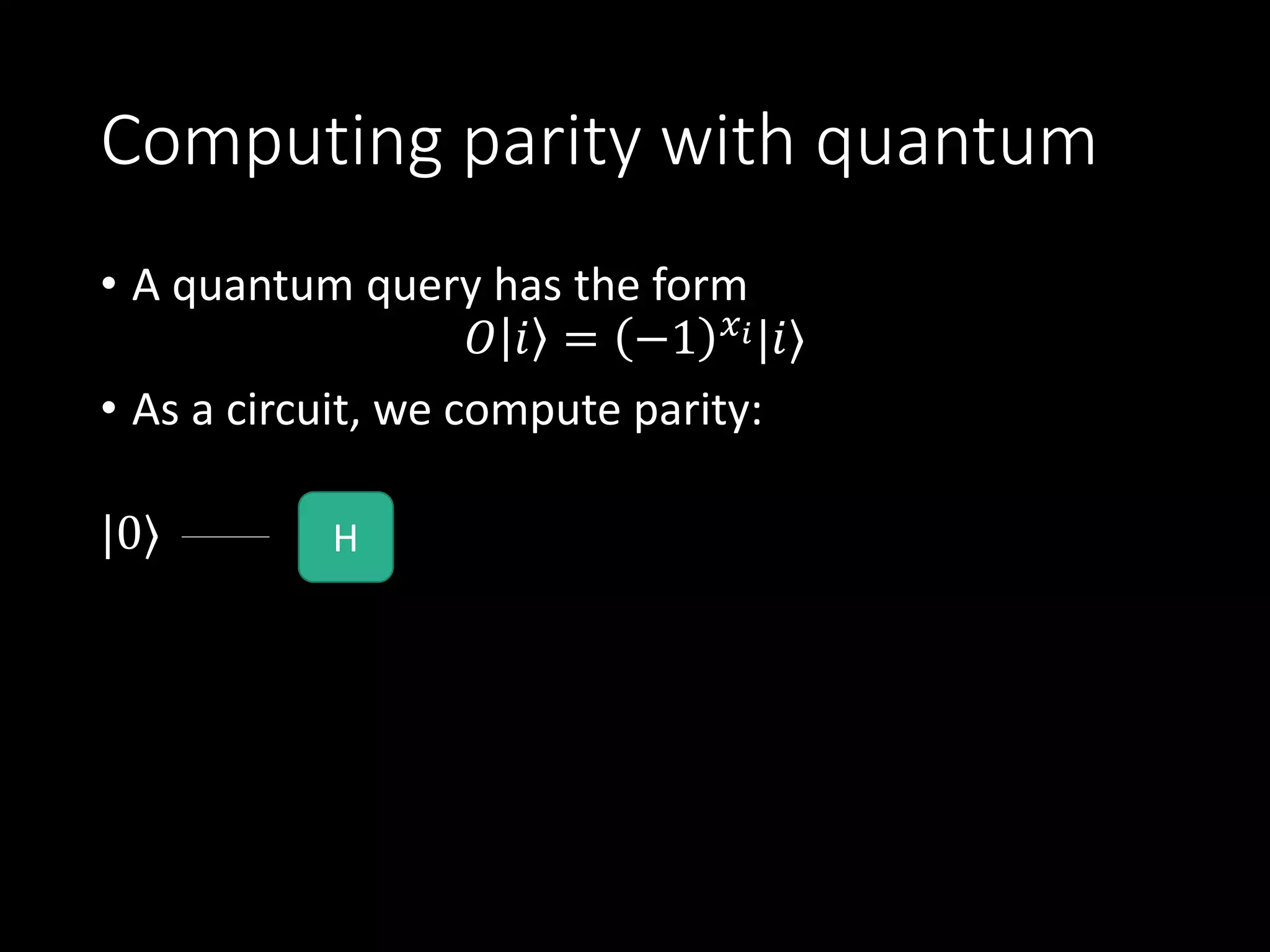
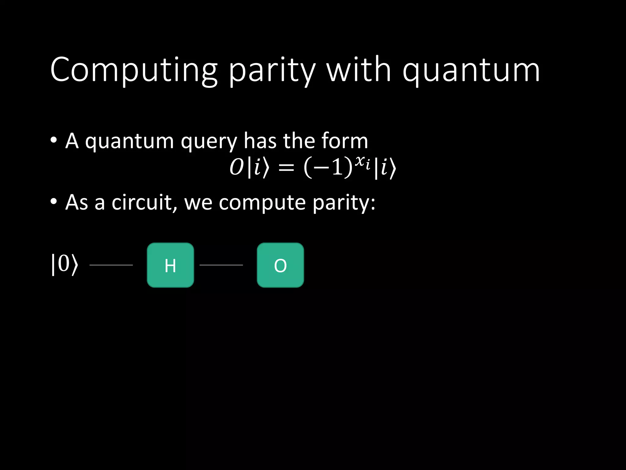
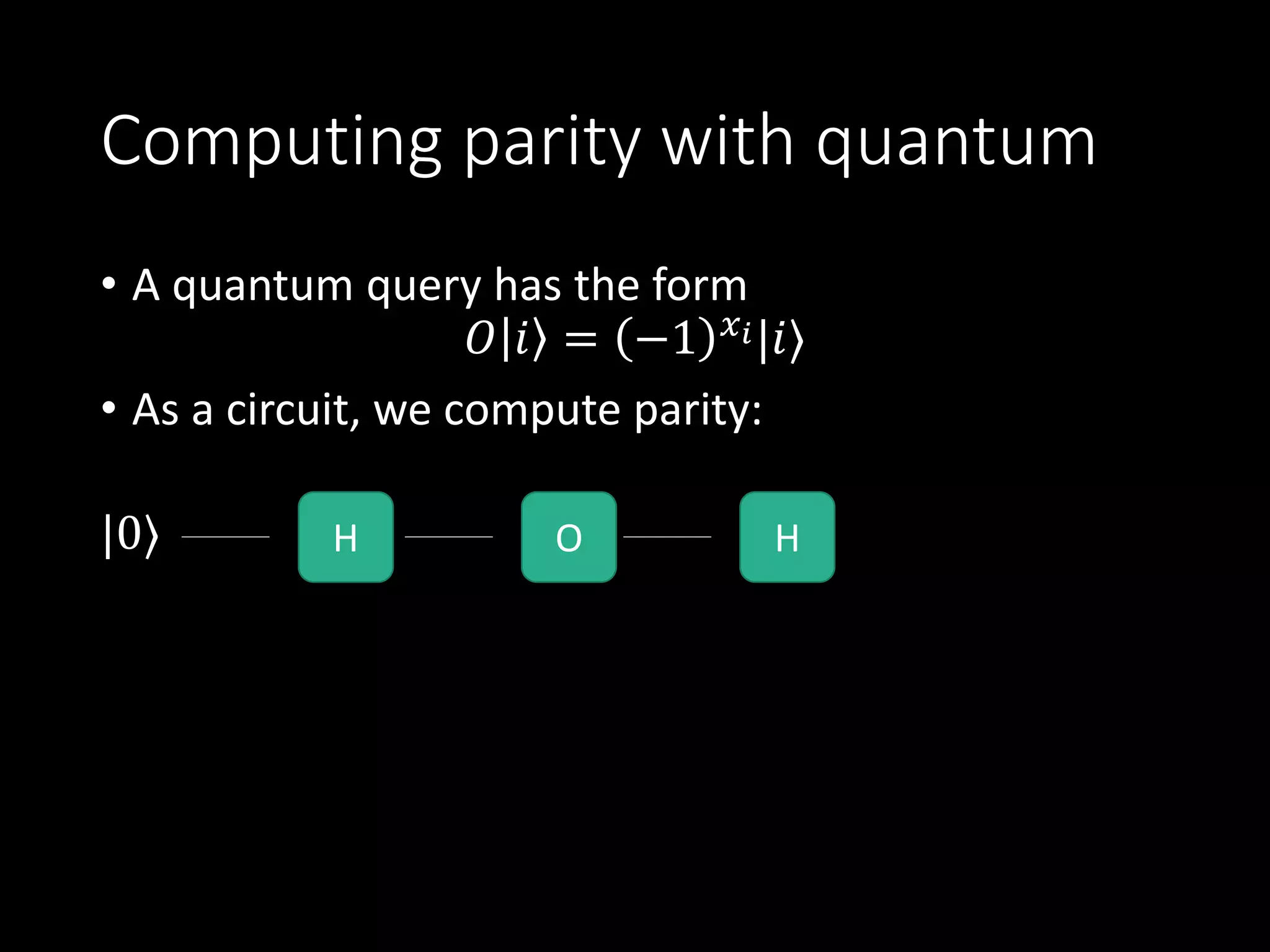
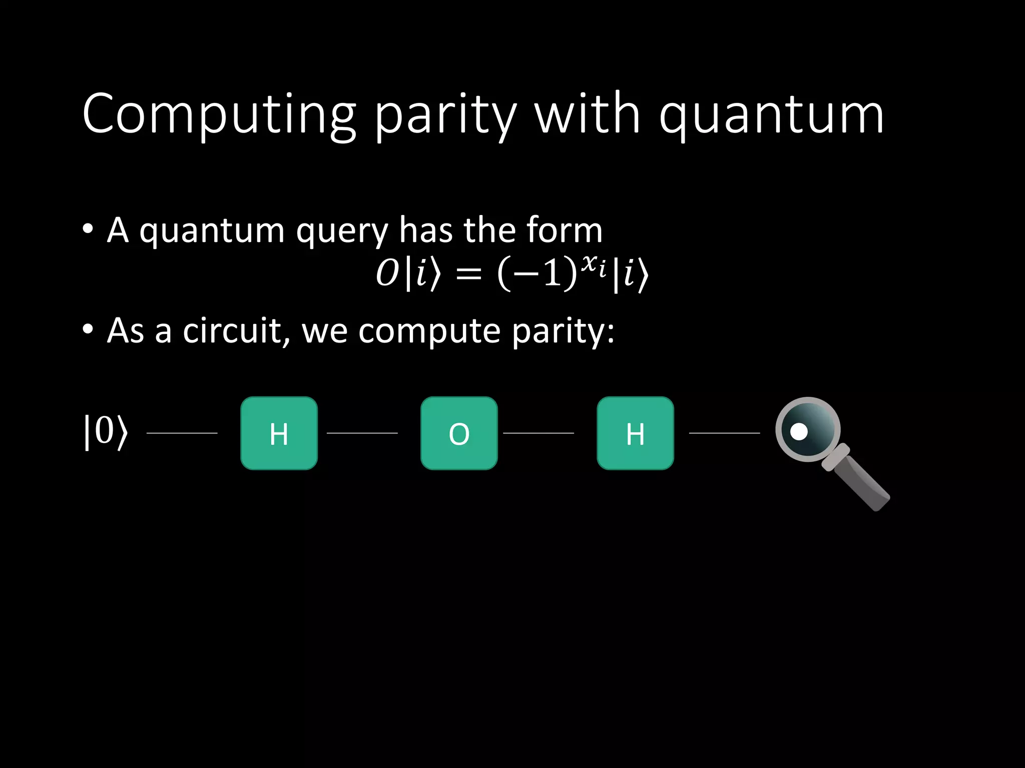
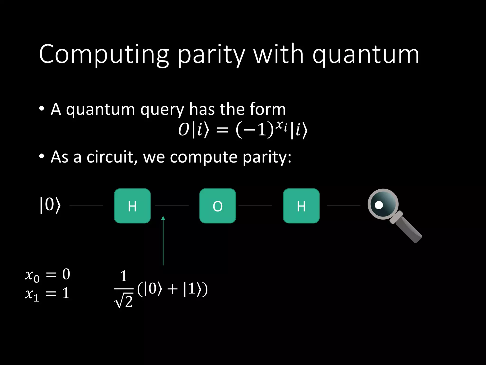
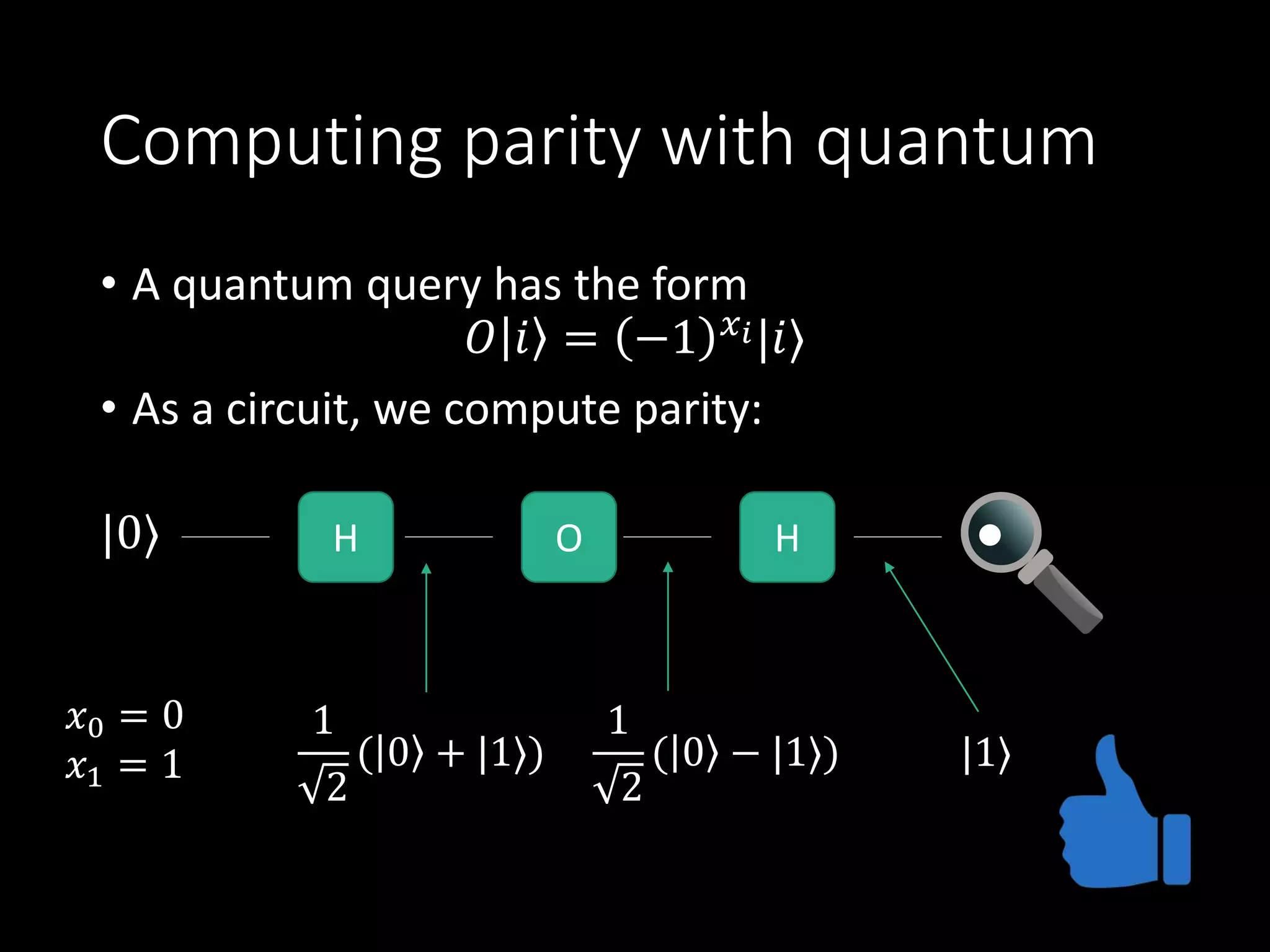
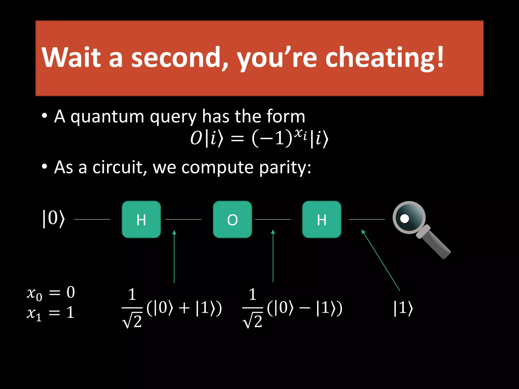
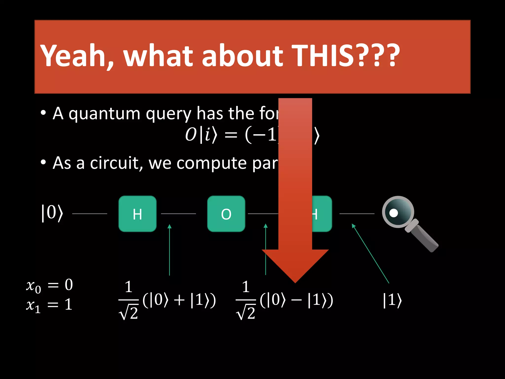
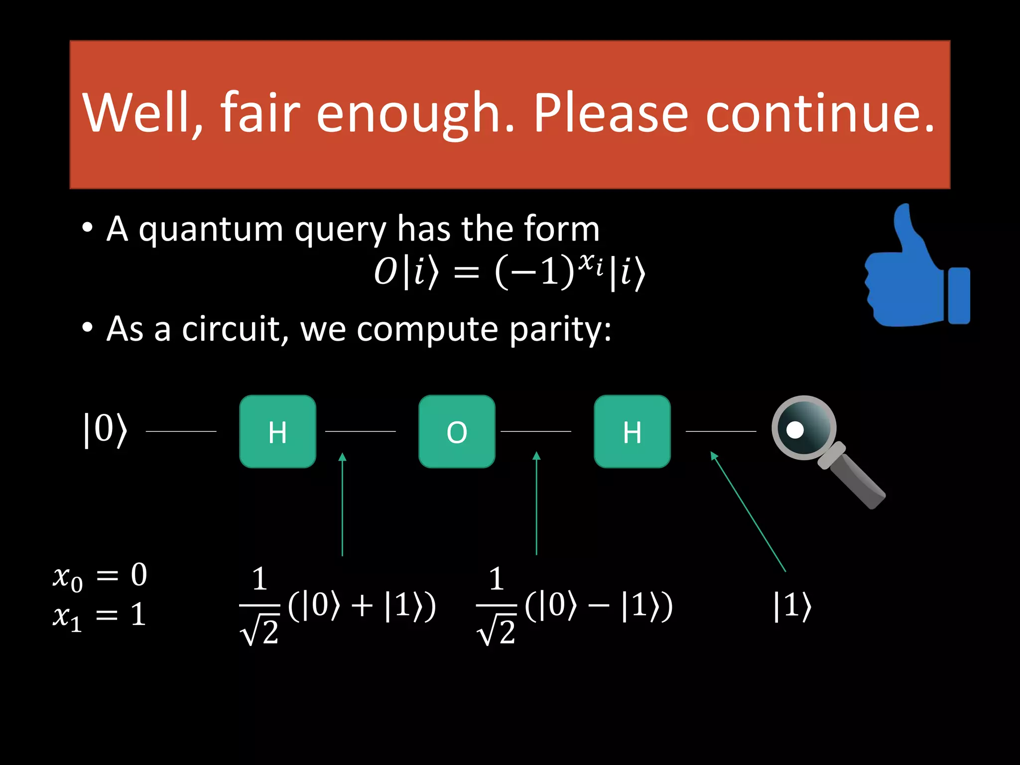
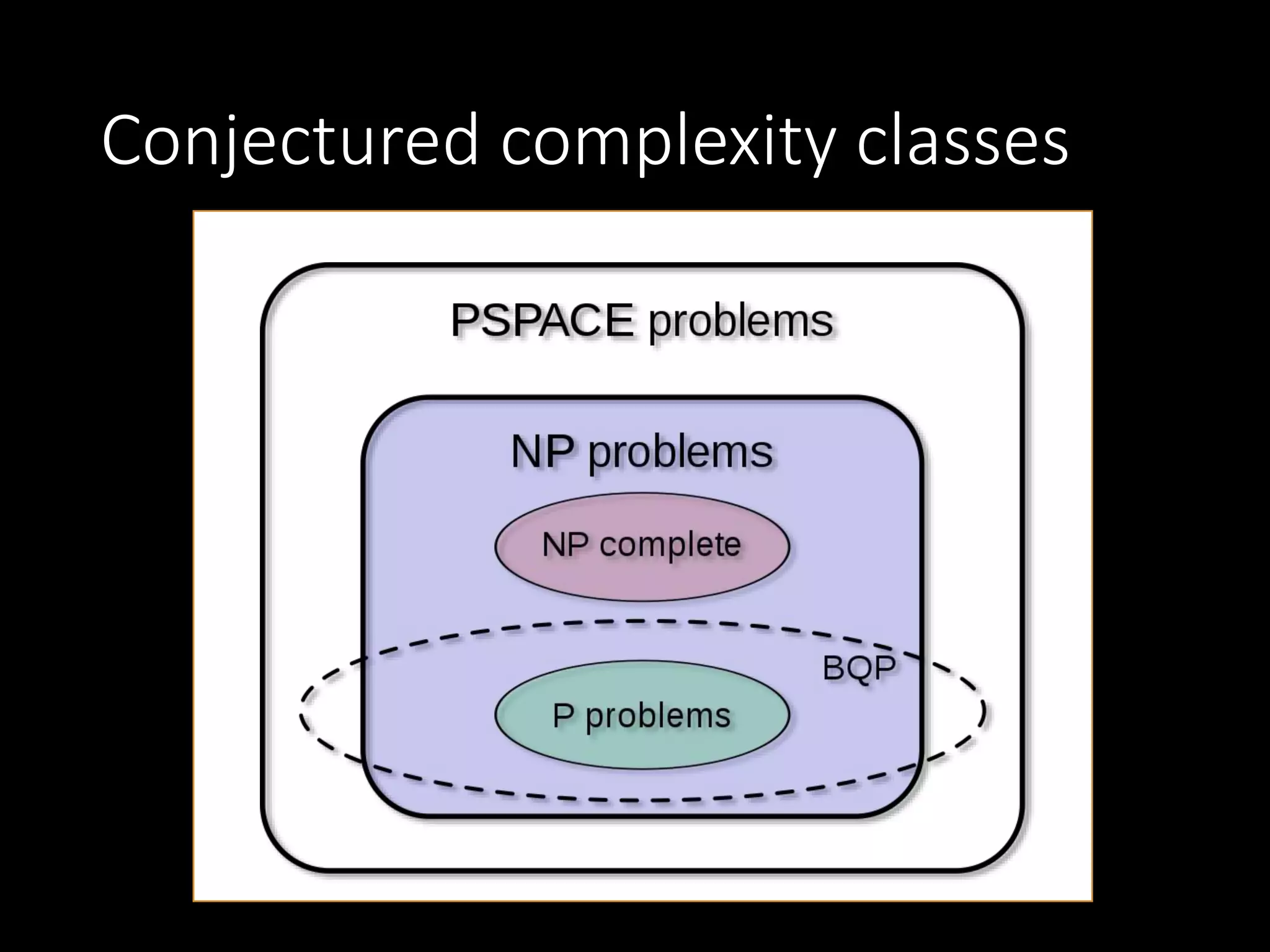
Introduces a discussion on quantum computers' power compared to classical ones, focusing on the parity function.
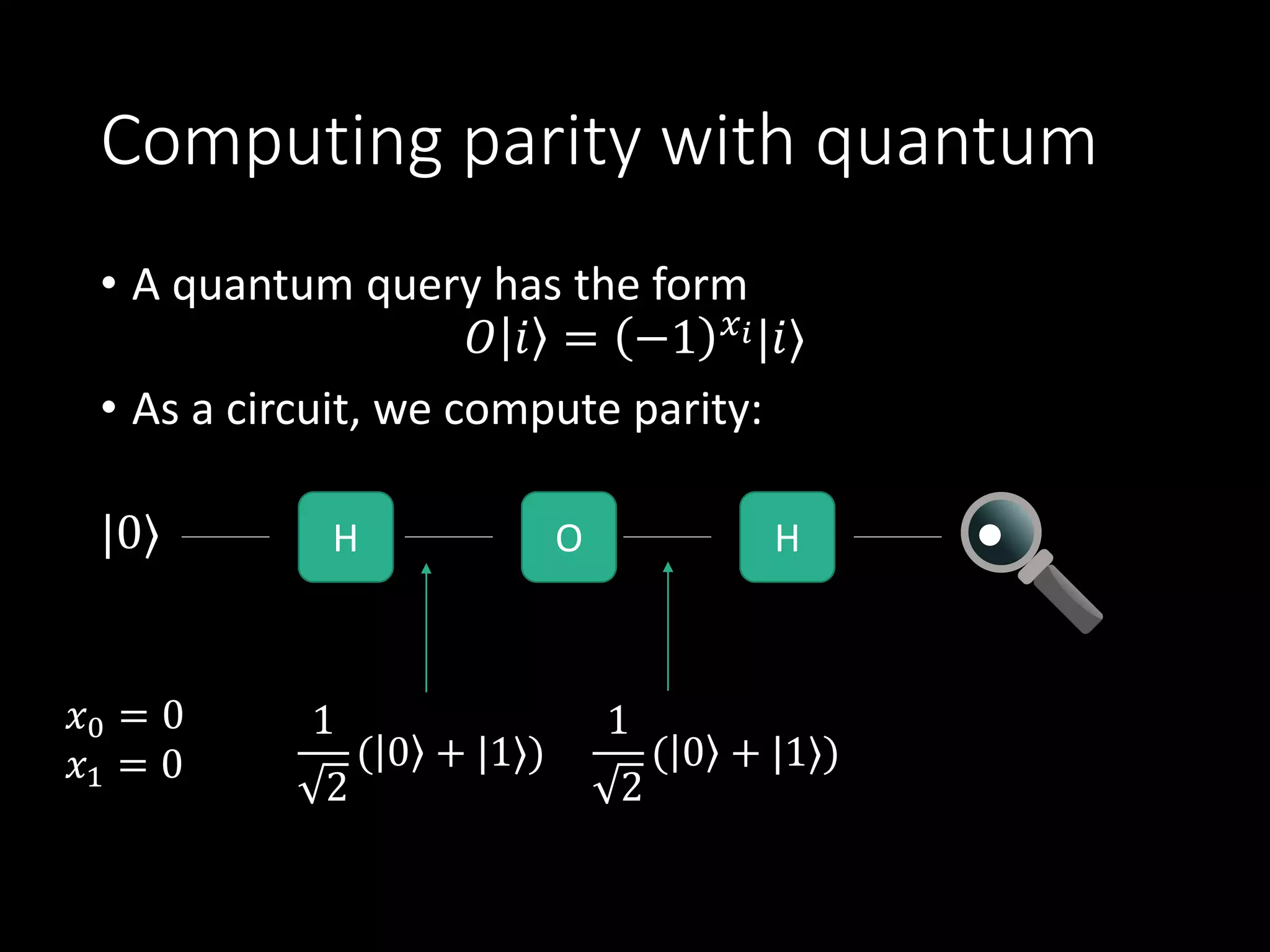
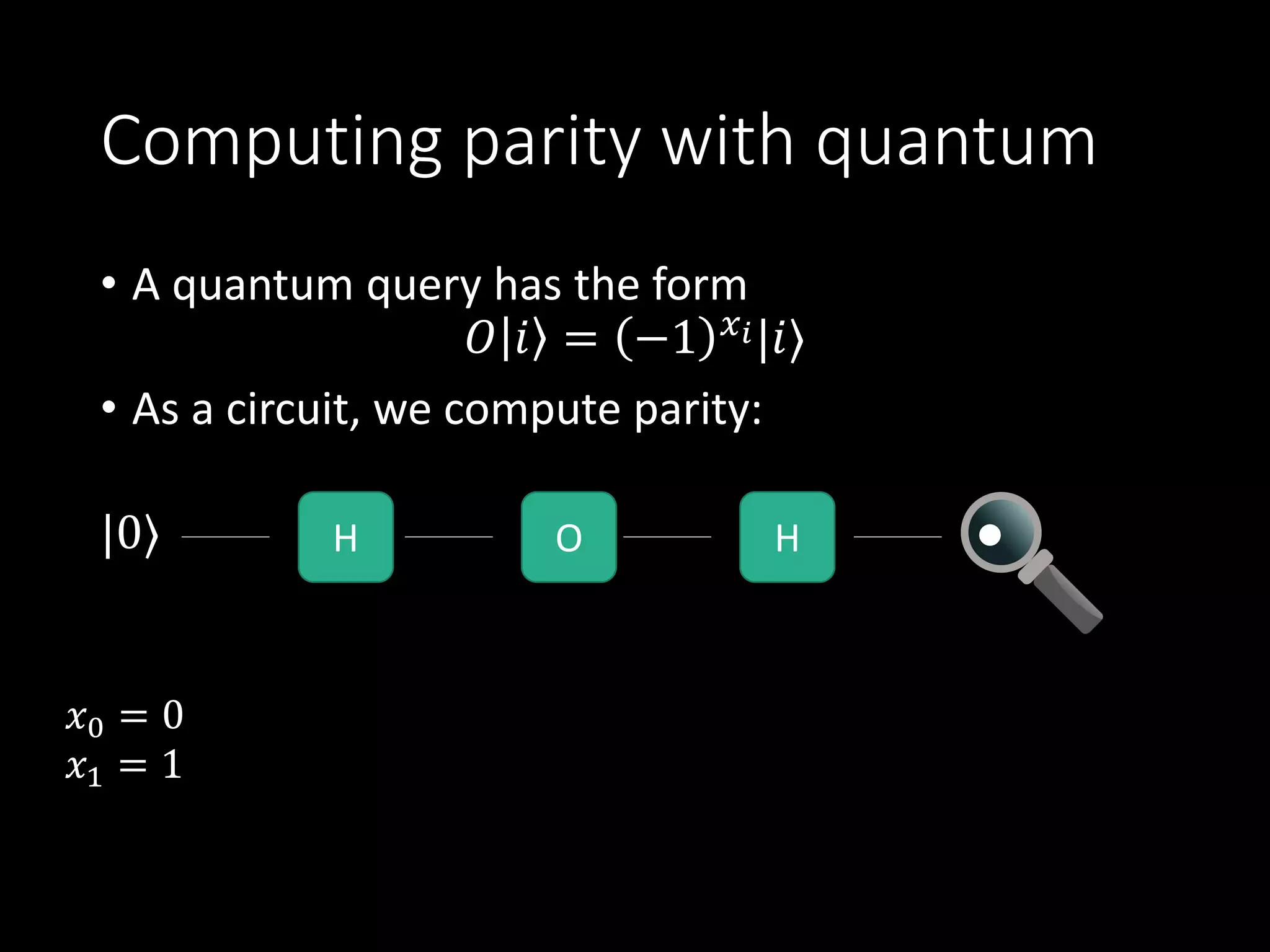
Explains how quantum computations for parity function are executed, including circuits and queries.
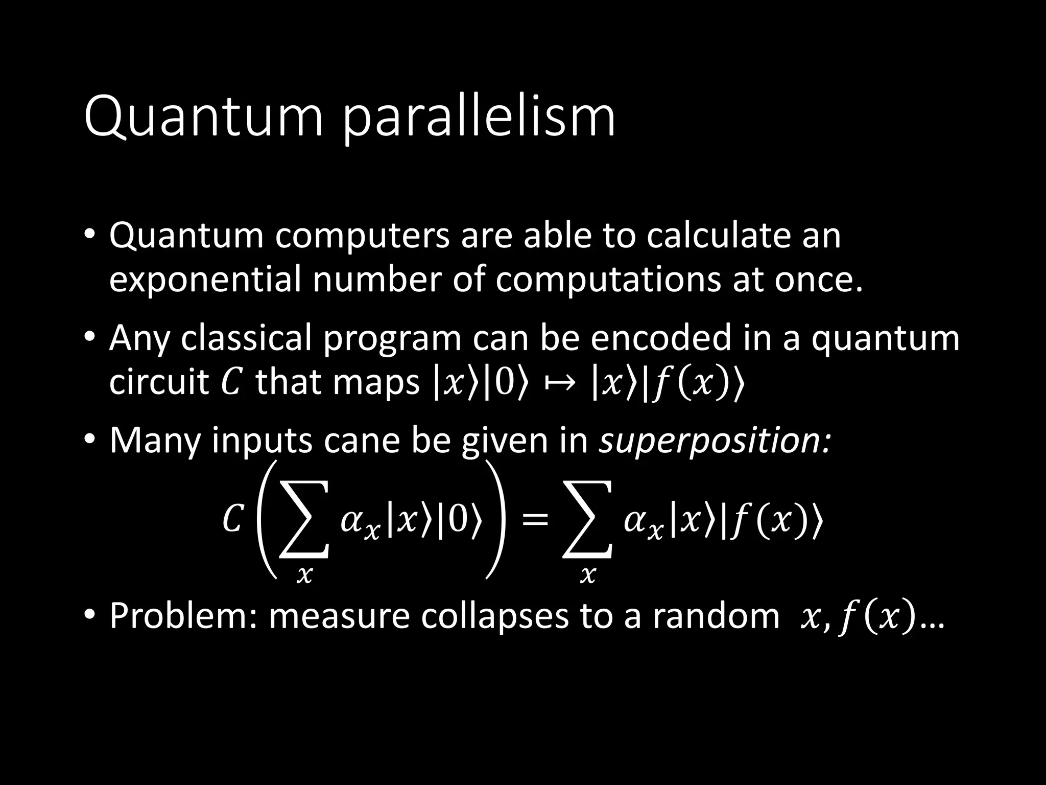
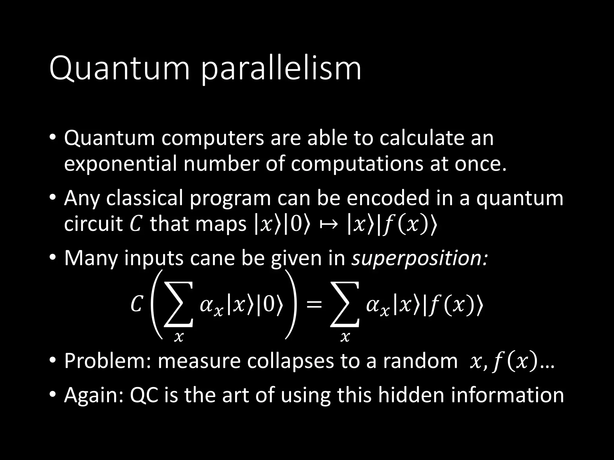
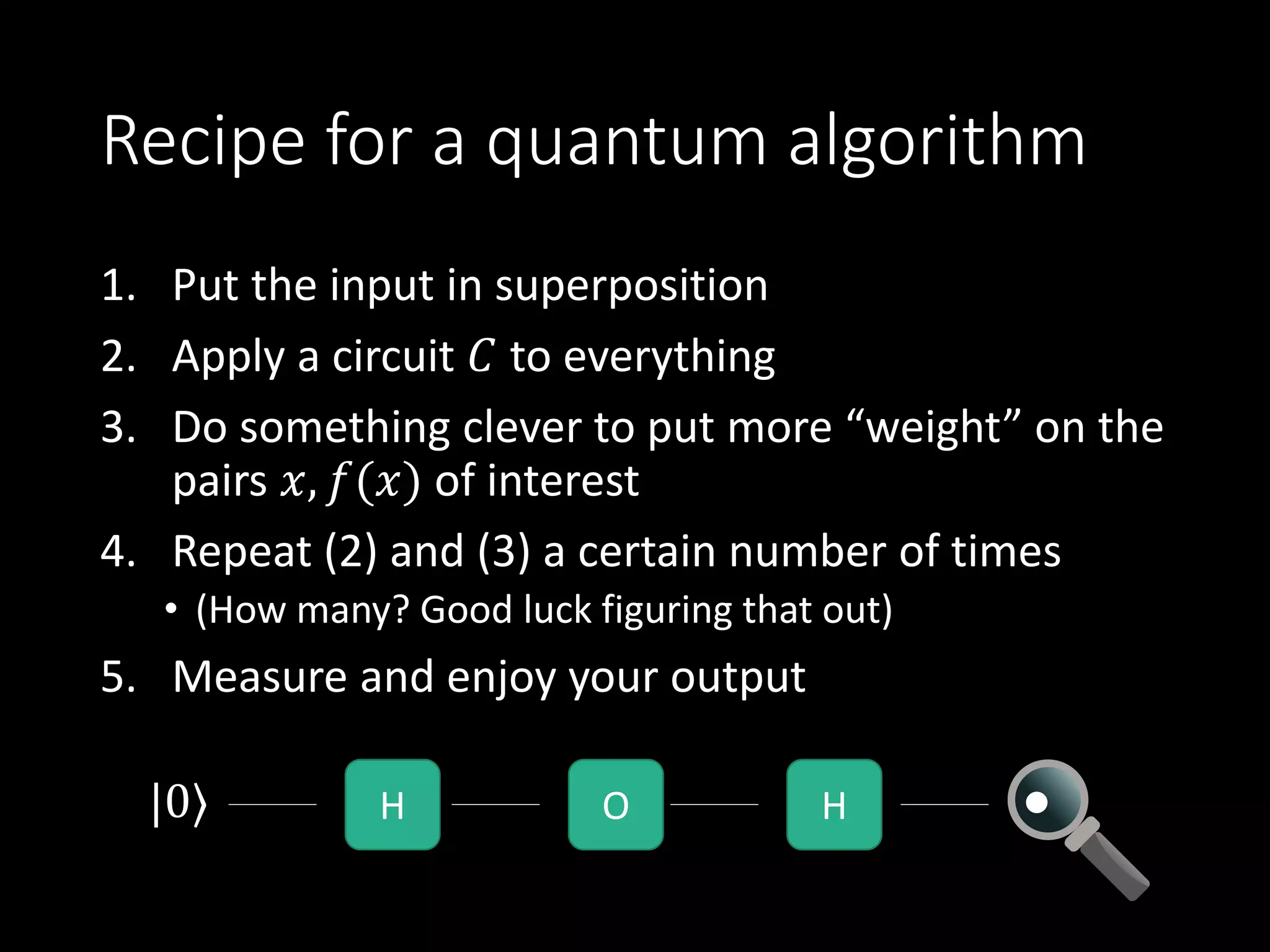
Describes how quantum computers can process many computations simultaneously and the concept of superposition.
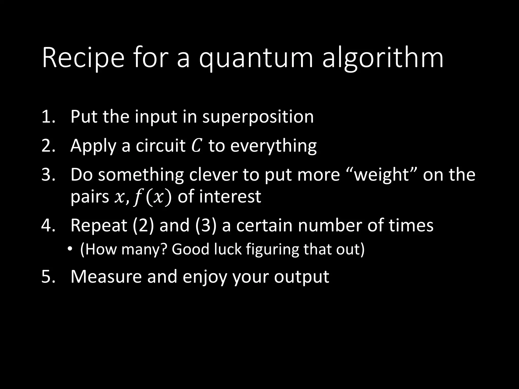
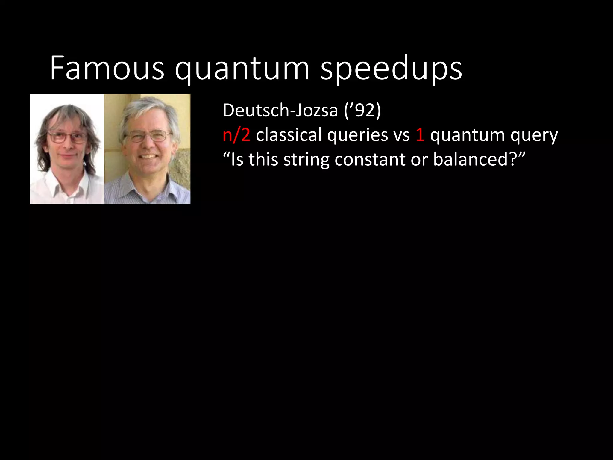
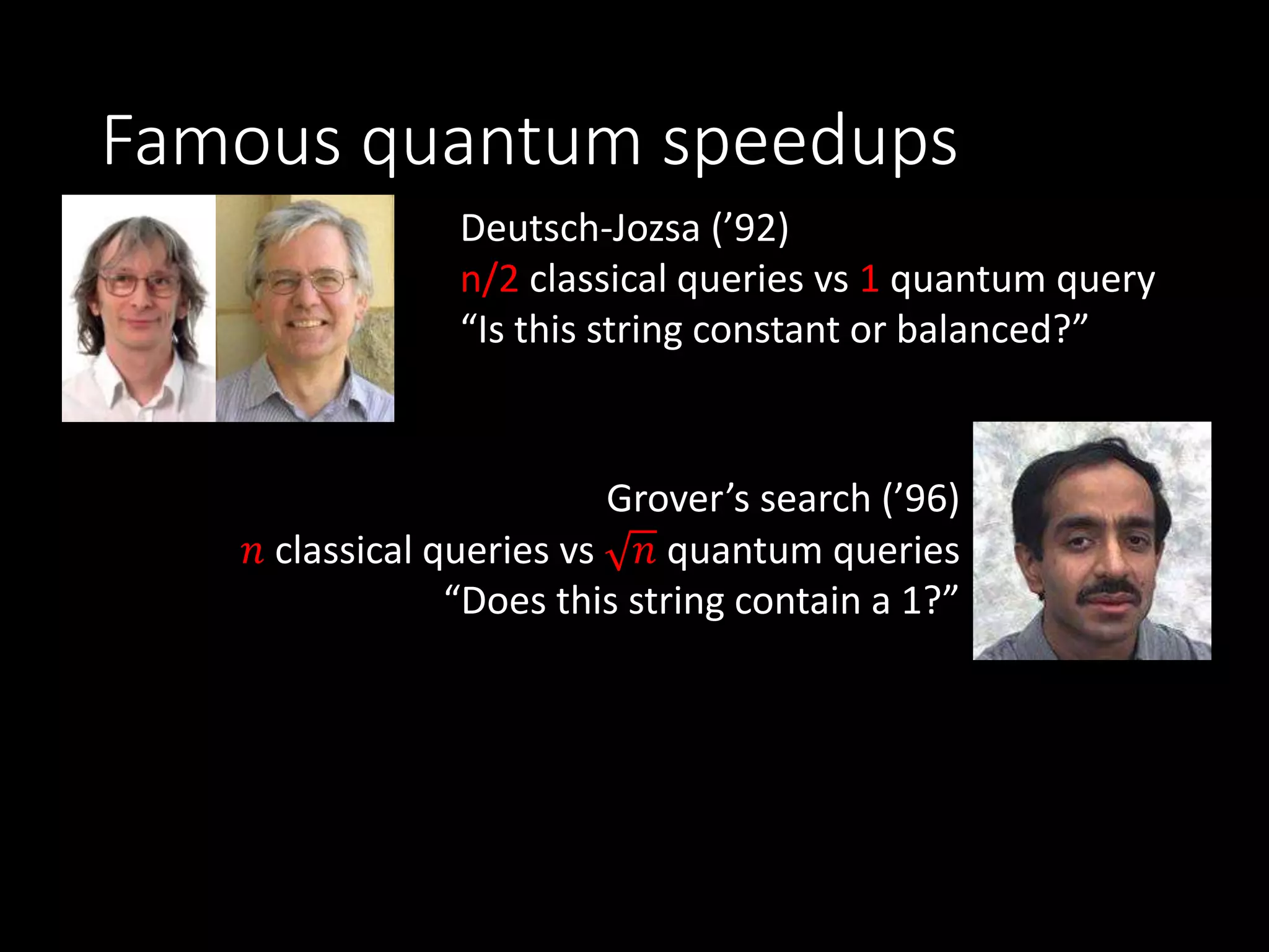
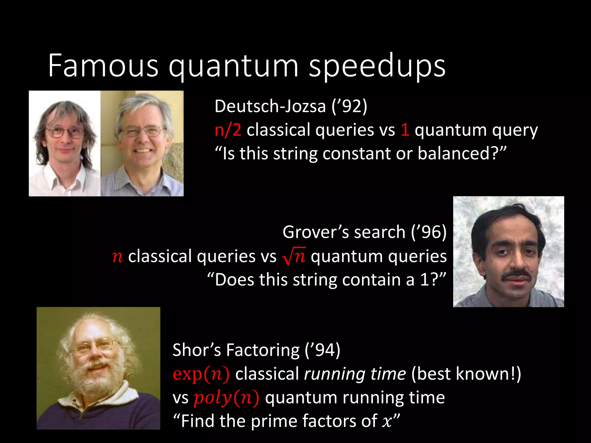
Highlights notable quantum algorithms like Deutsch-Jozsa, Grover’s search, and Shor’s algorithm, comparing classical vs quantum performance.
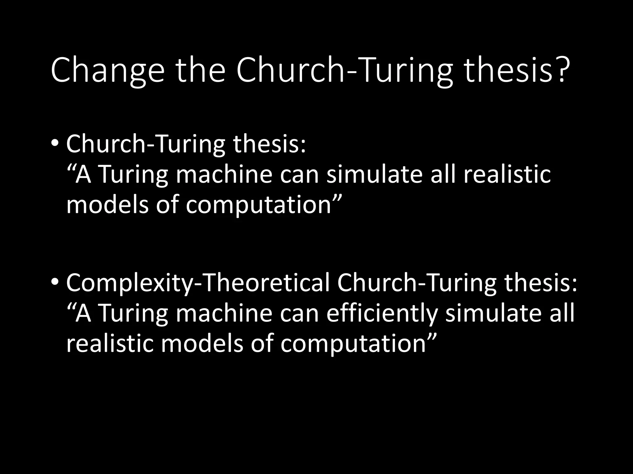
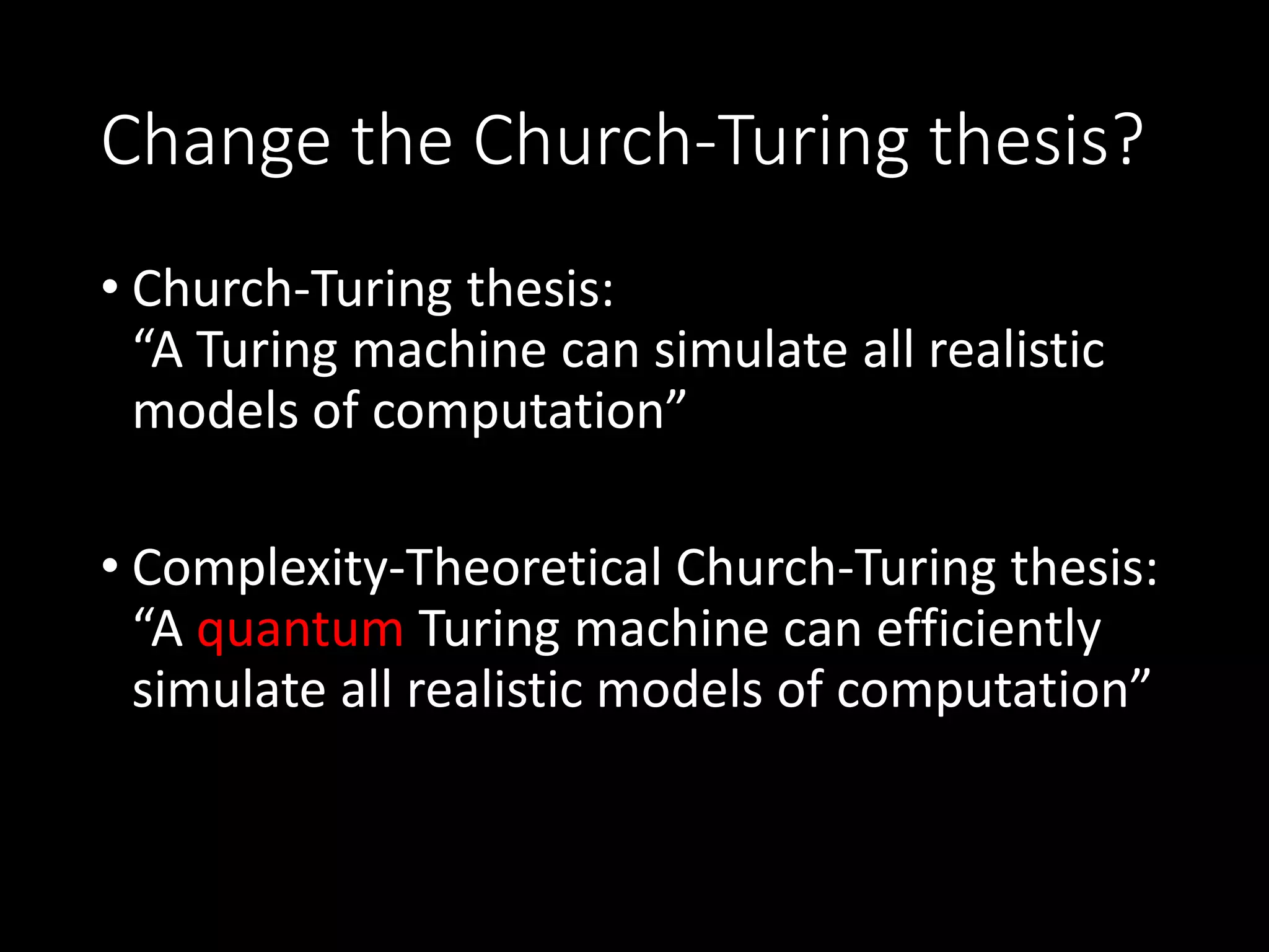
Discusses implications for the Church-Turing thesis within the context of quantum computing.
Introduces quantum cryptography and its applications including certified randomness and detection of spy presence.
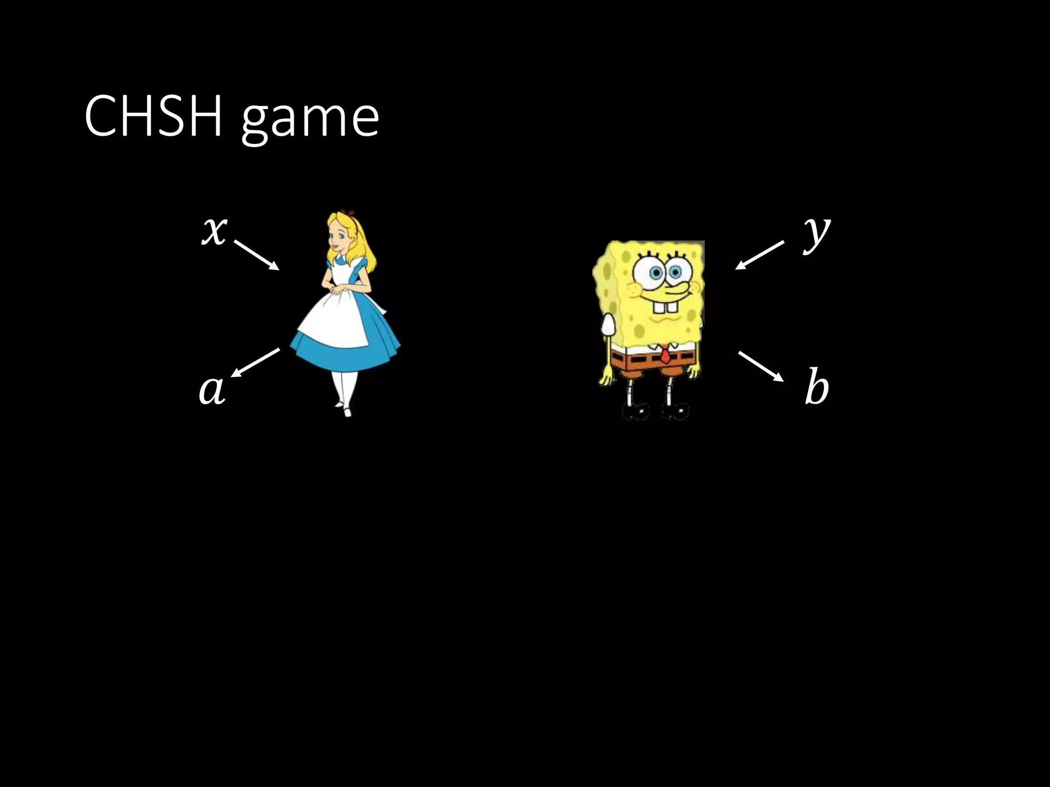
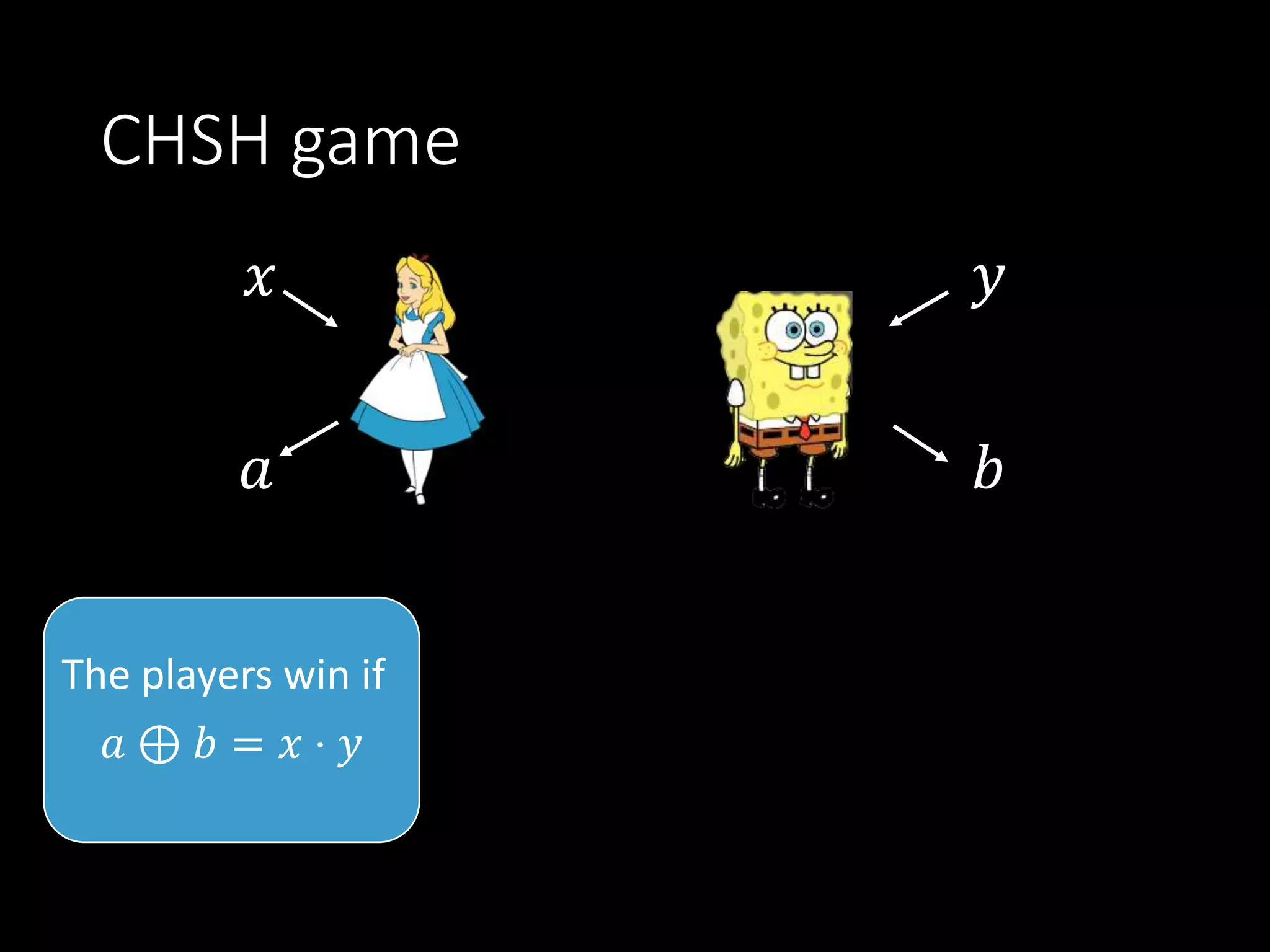
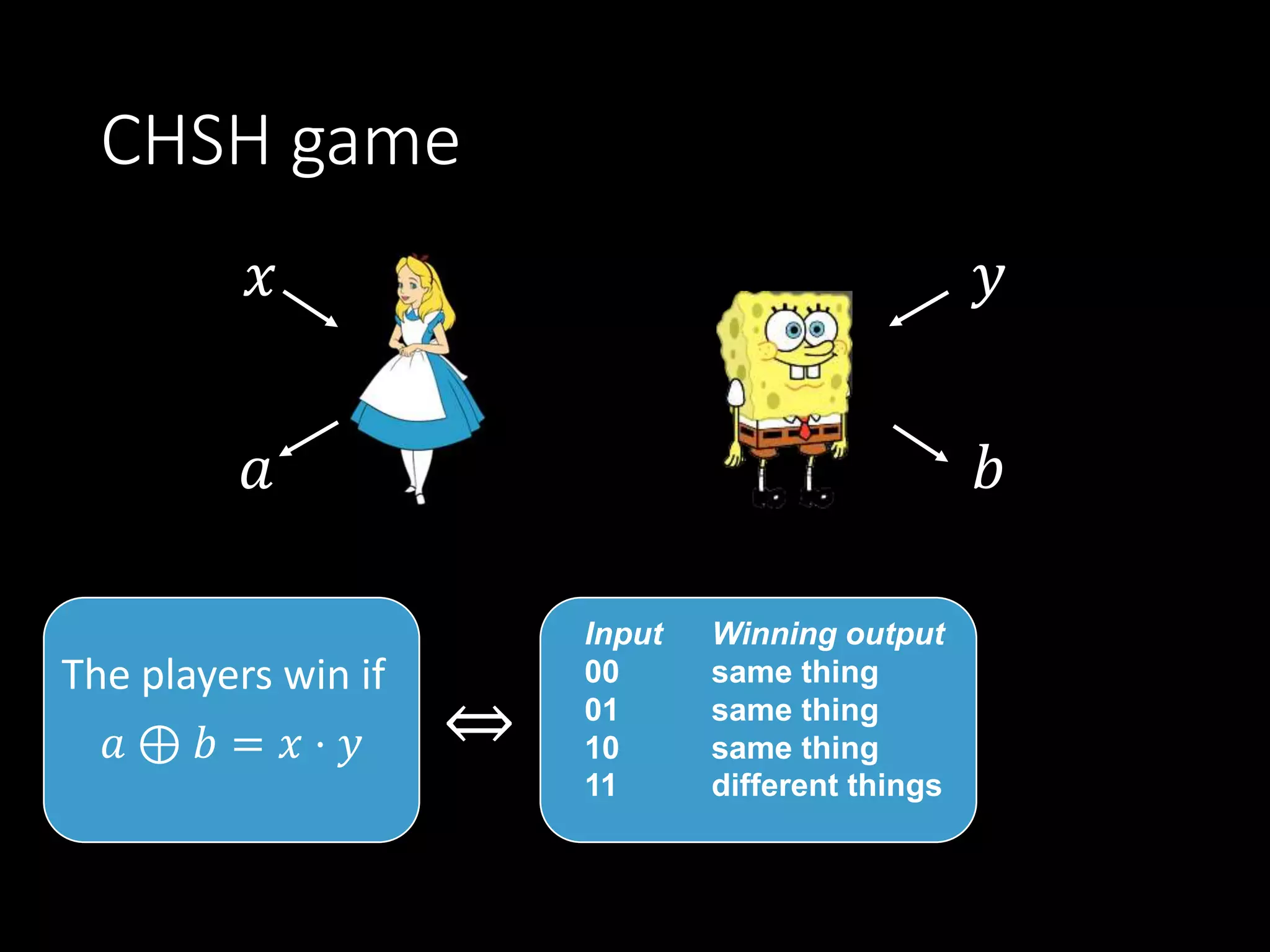
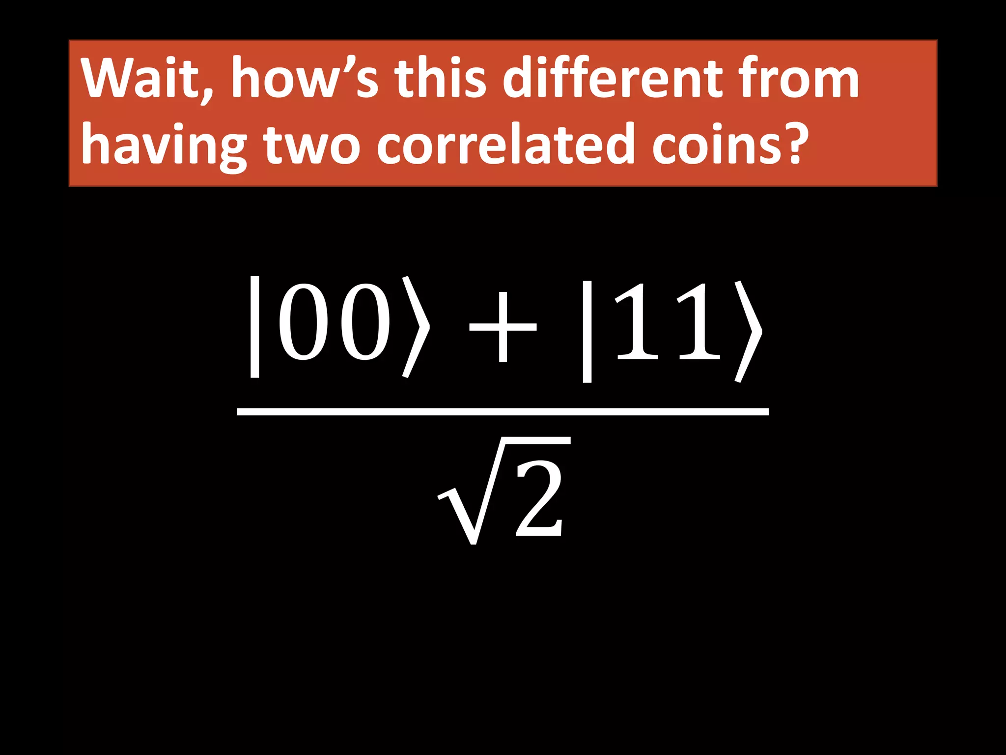
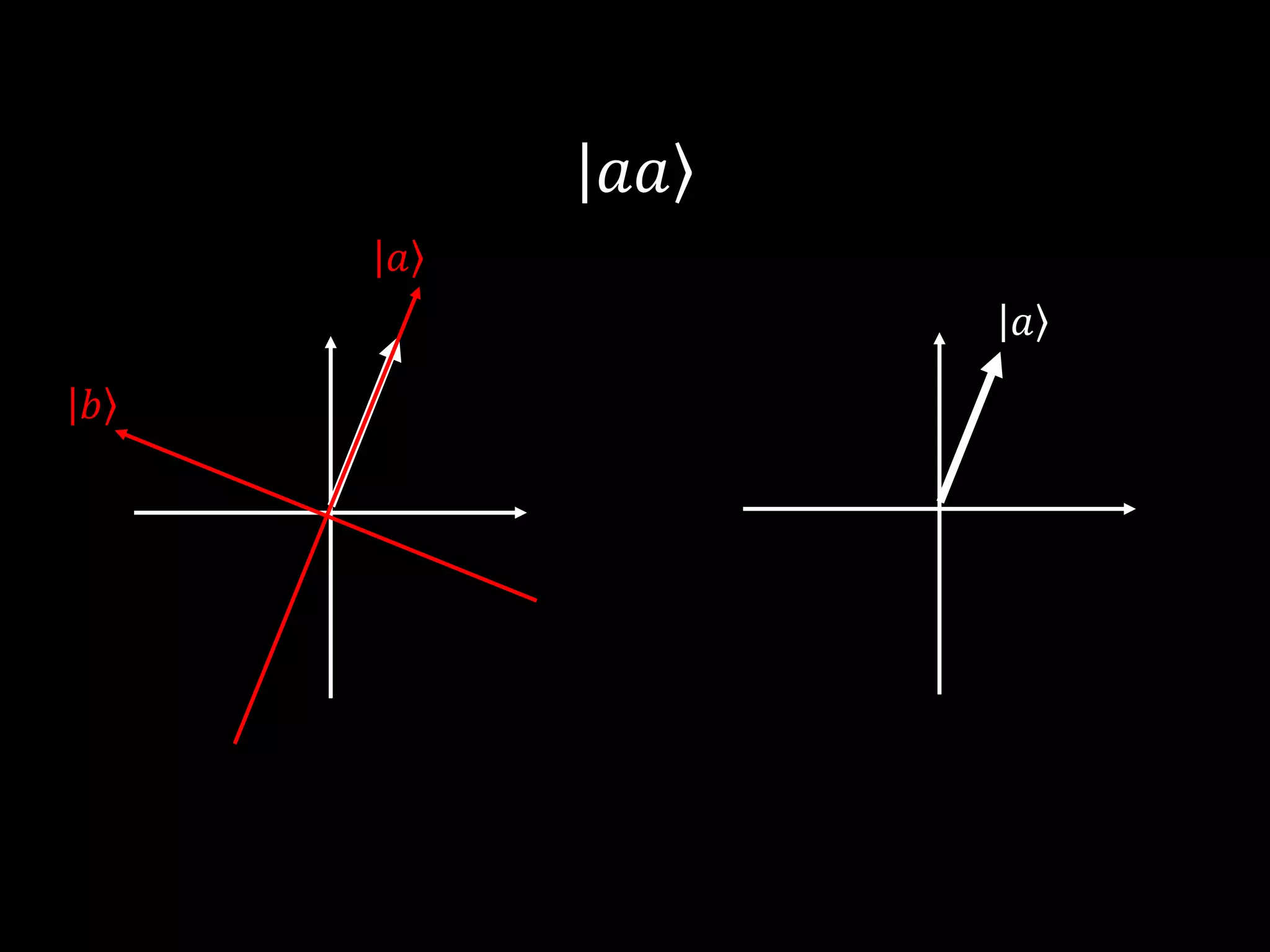
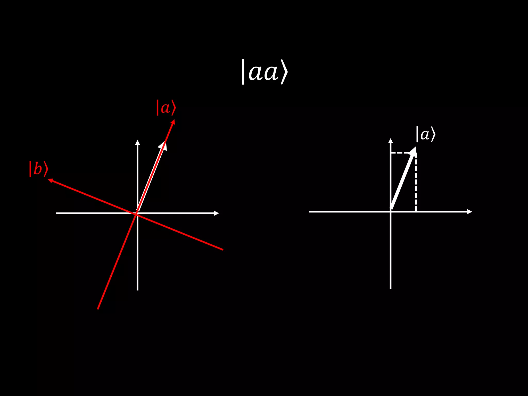
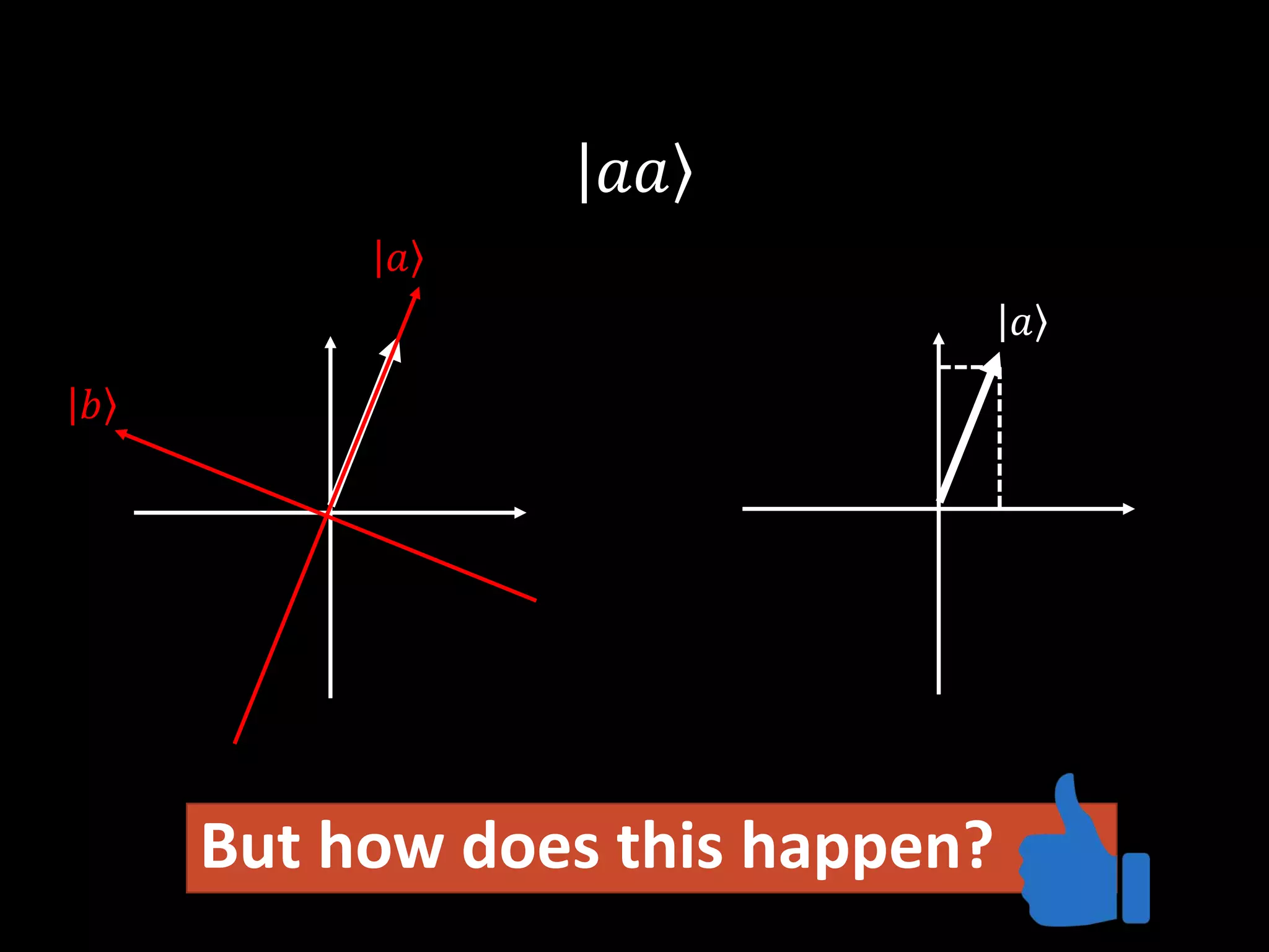
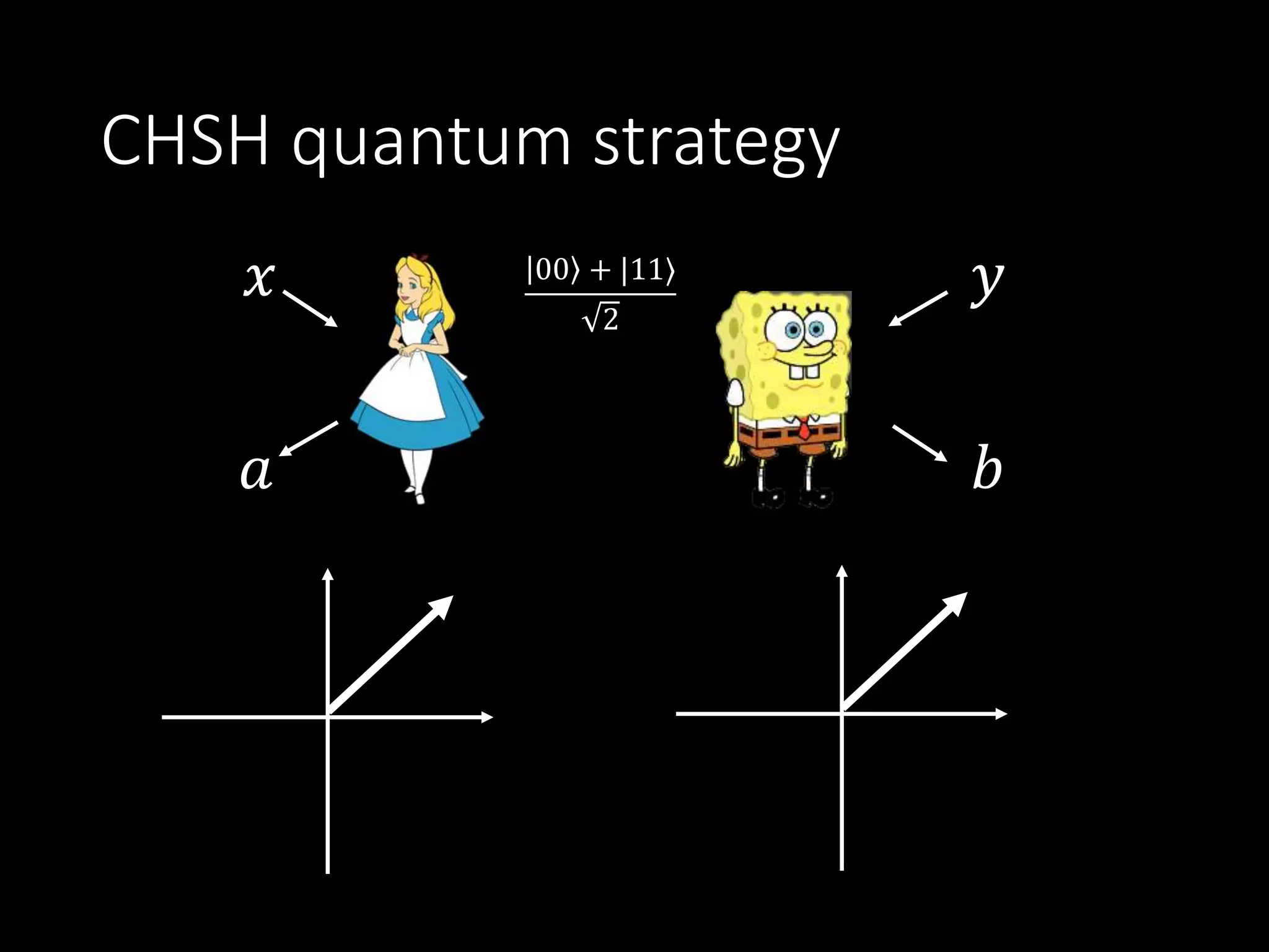
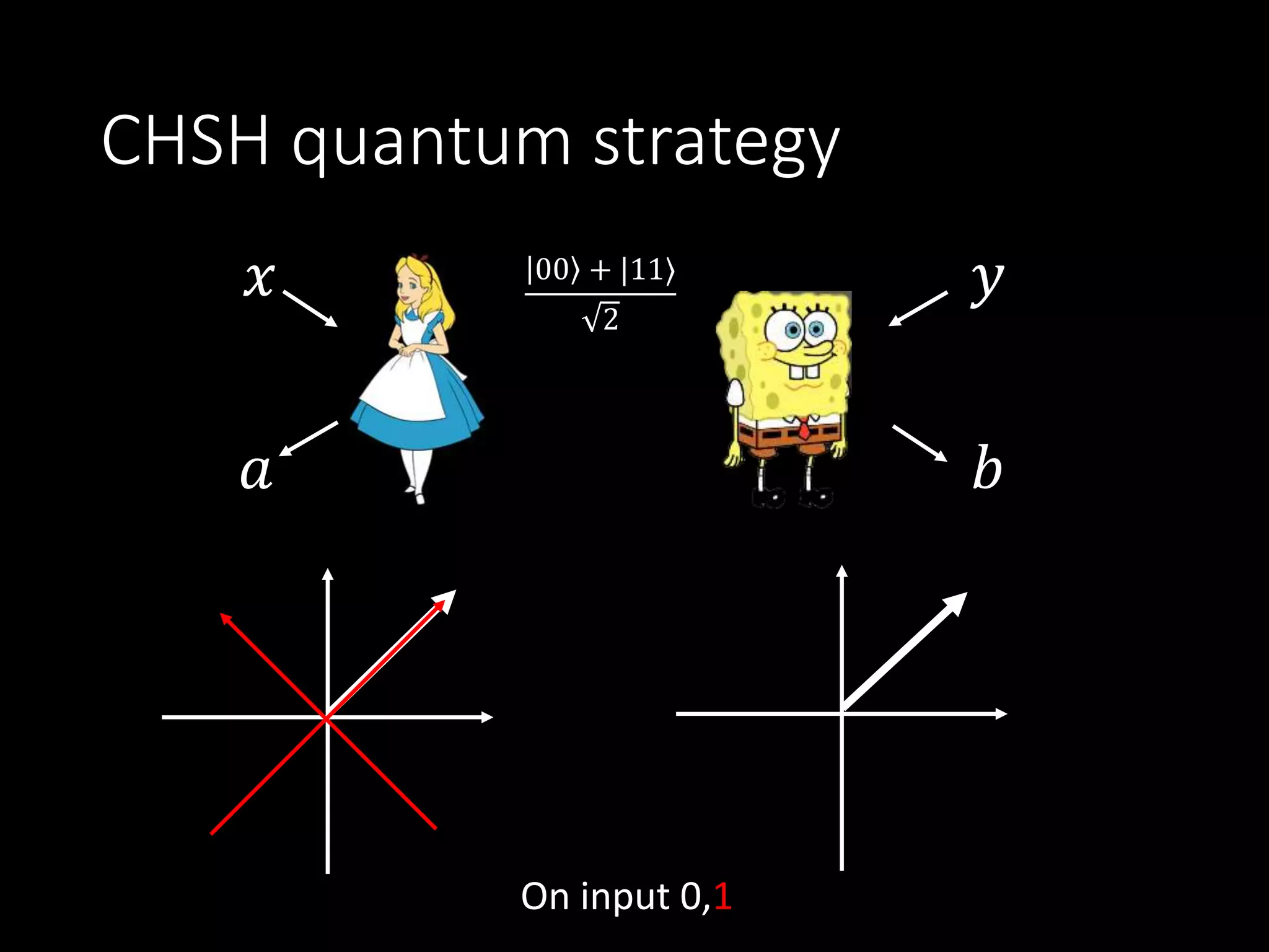
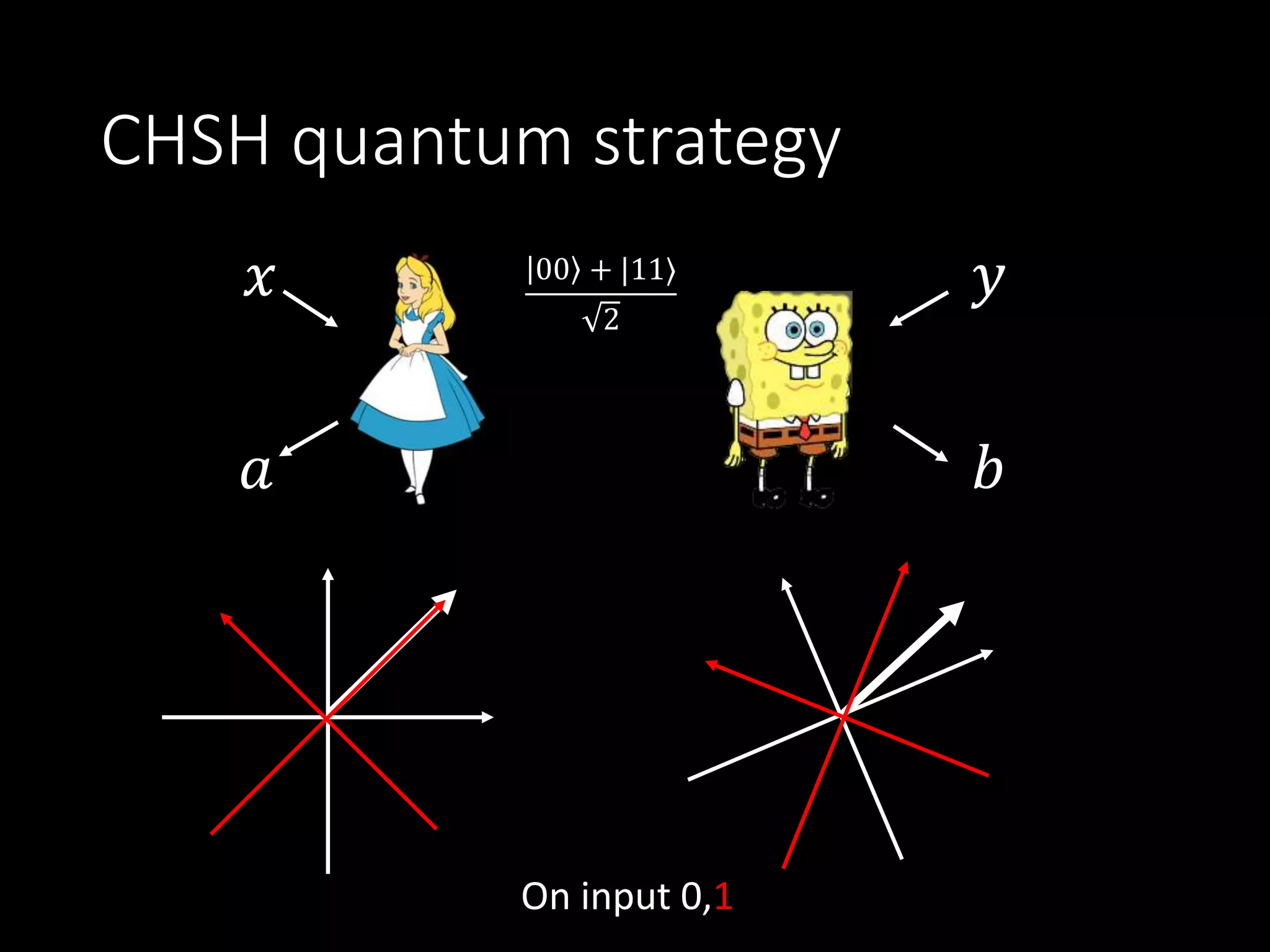
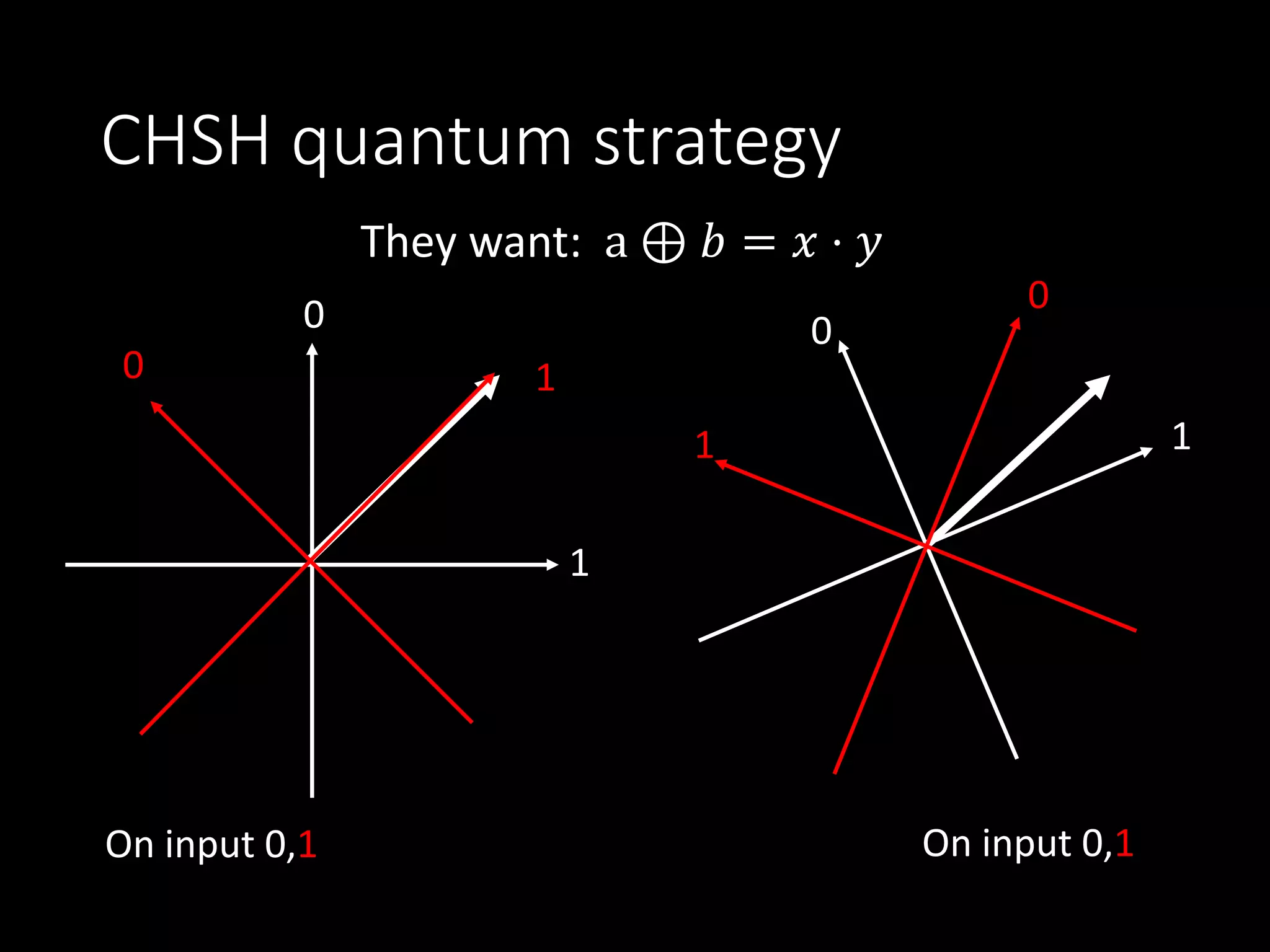
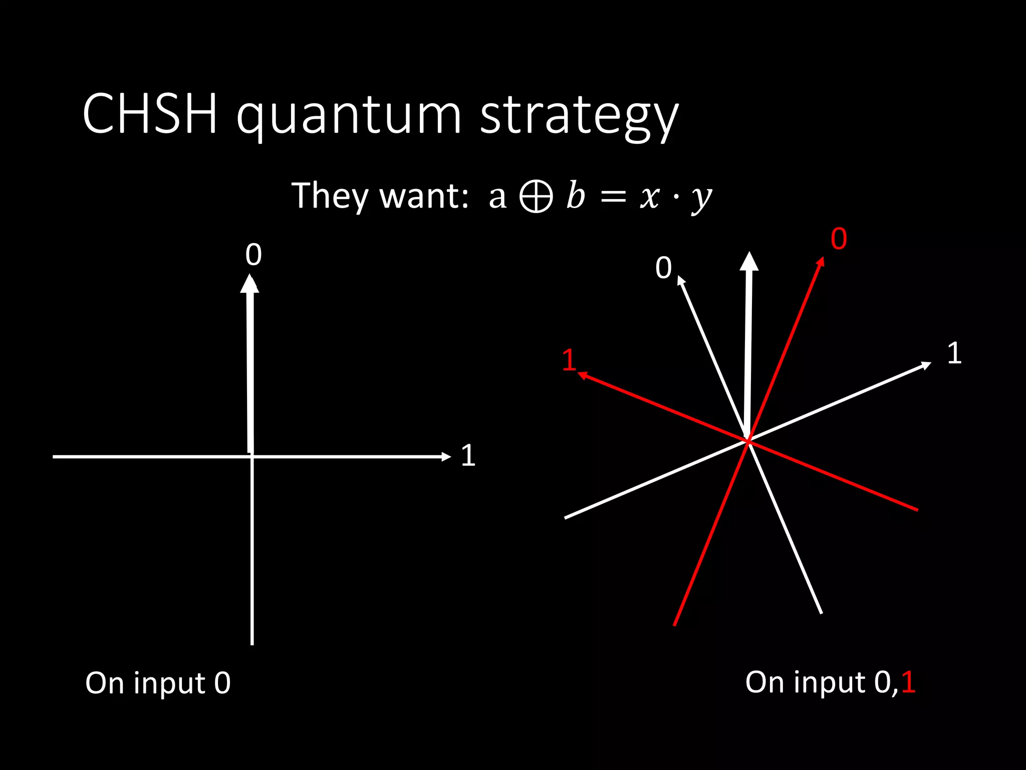
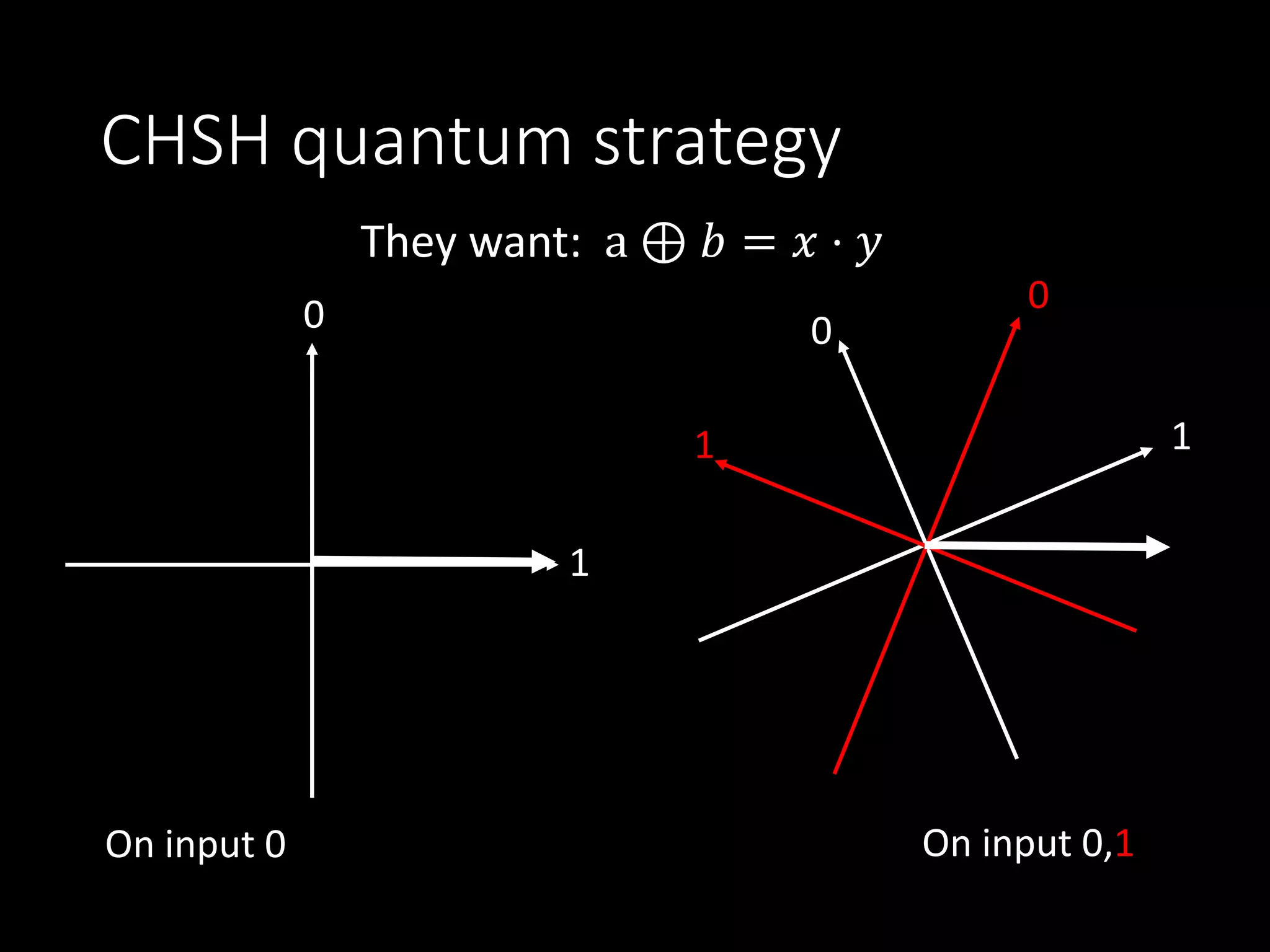
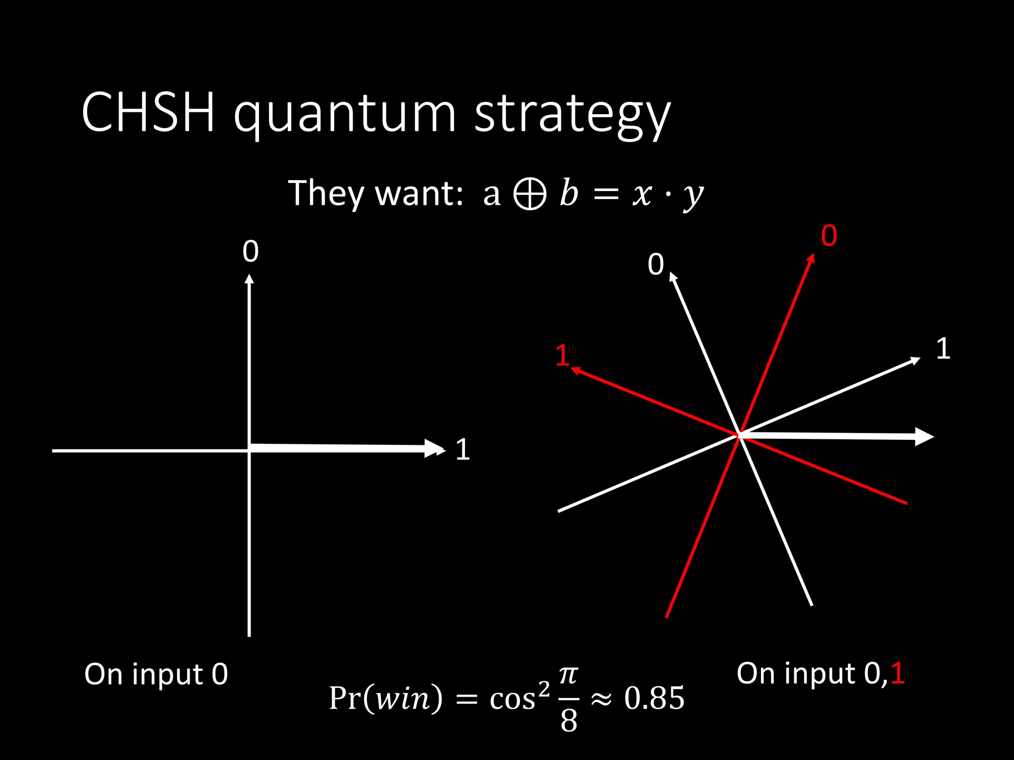
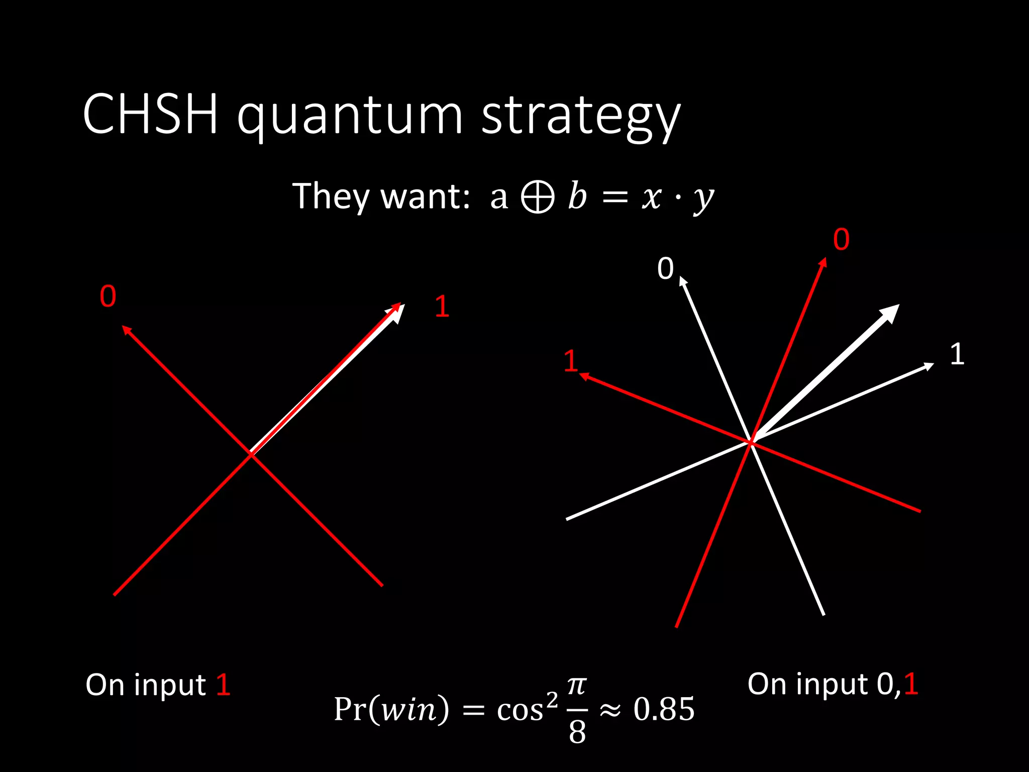
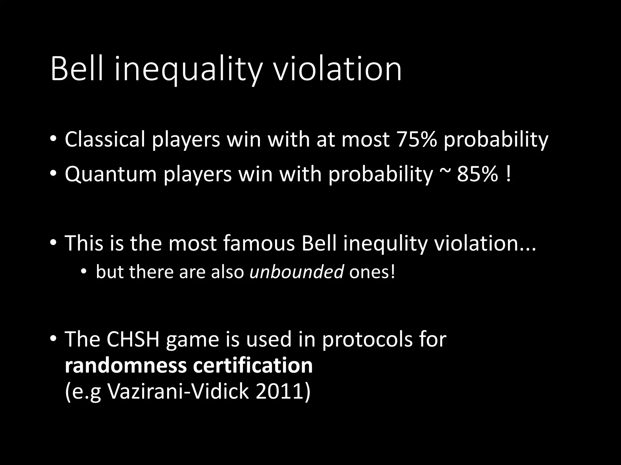
Explains non-locality in quantum mechanics, Bell inequalities, and the advantages of quantum players over classical.
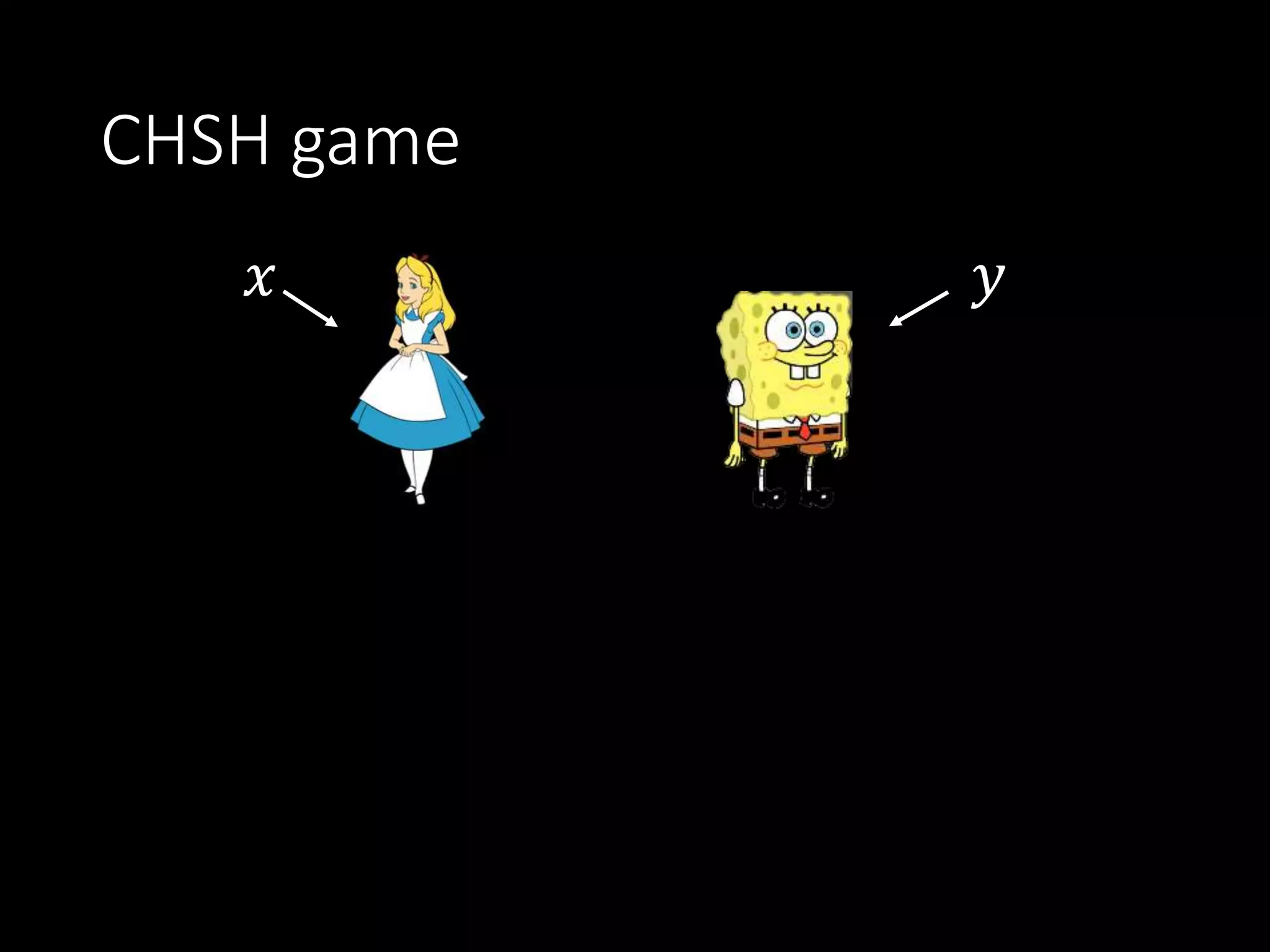
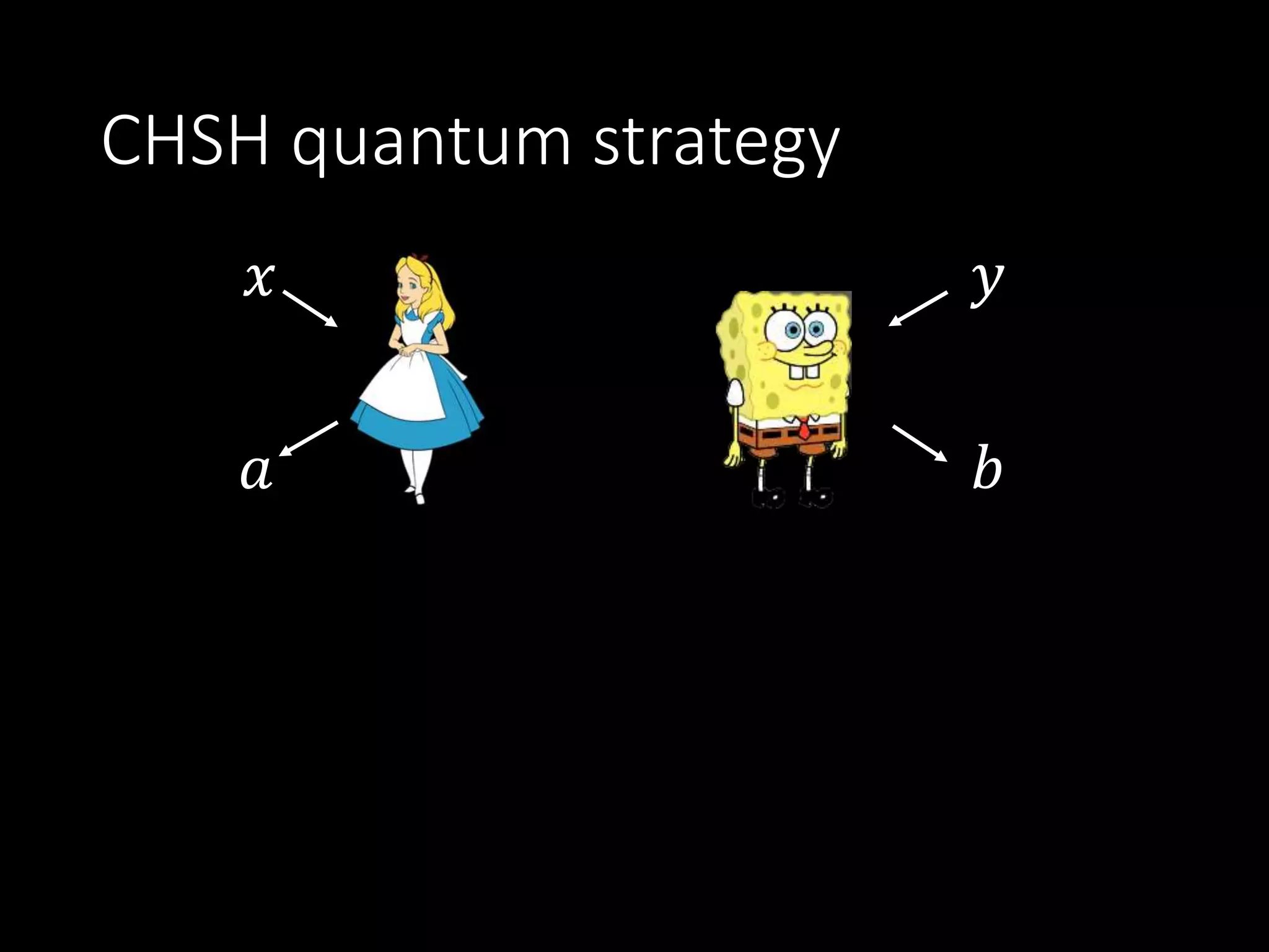
Details the gameplay mechanics of the CHSH game and calculations of winning probabilities for quantum vs classical players.
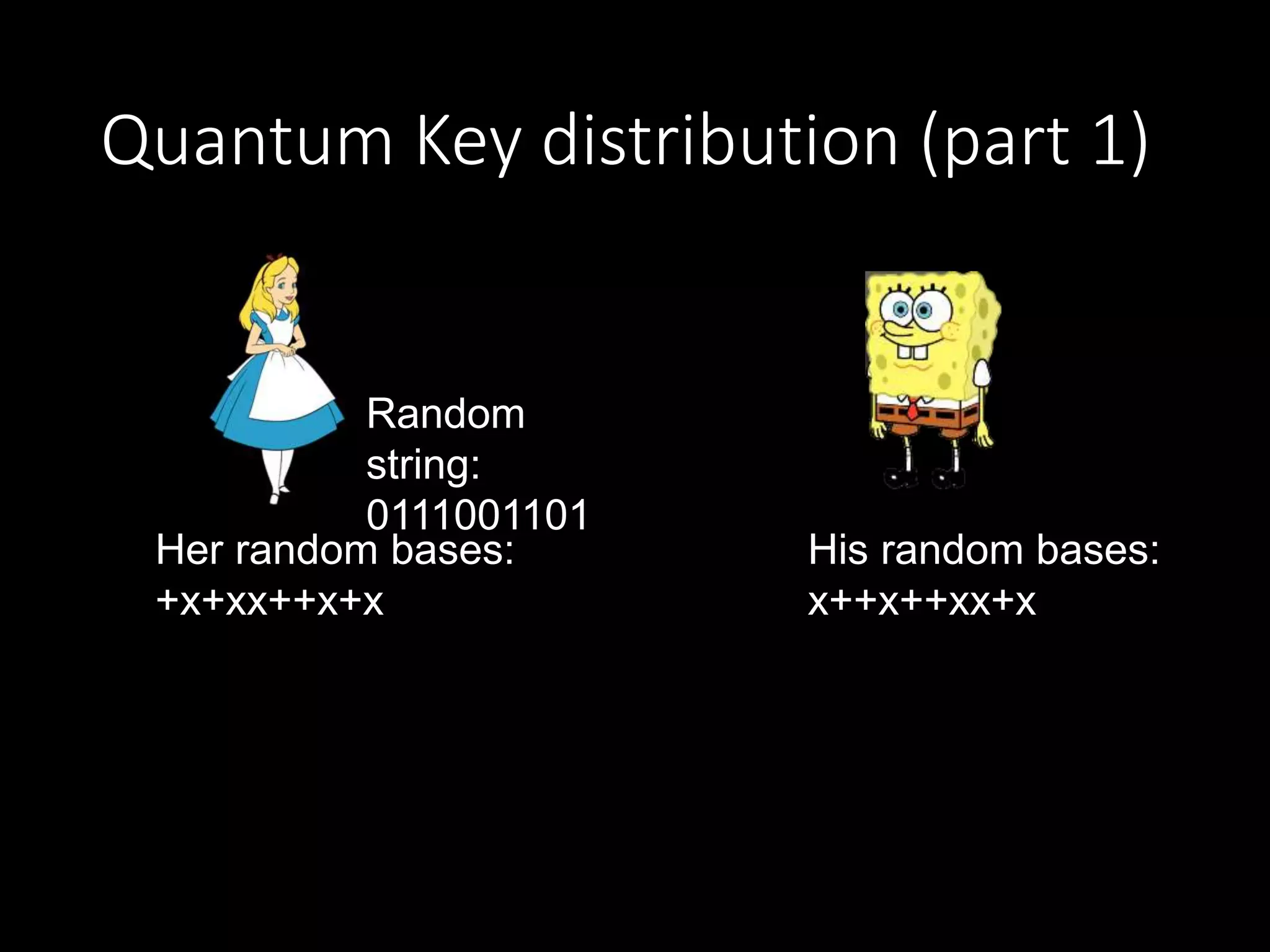
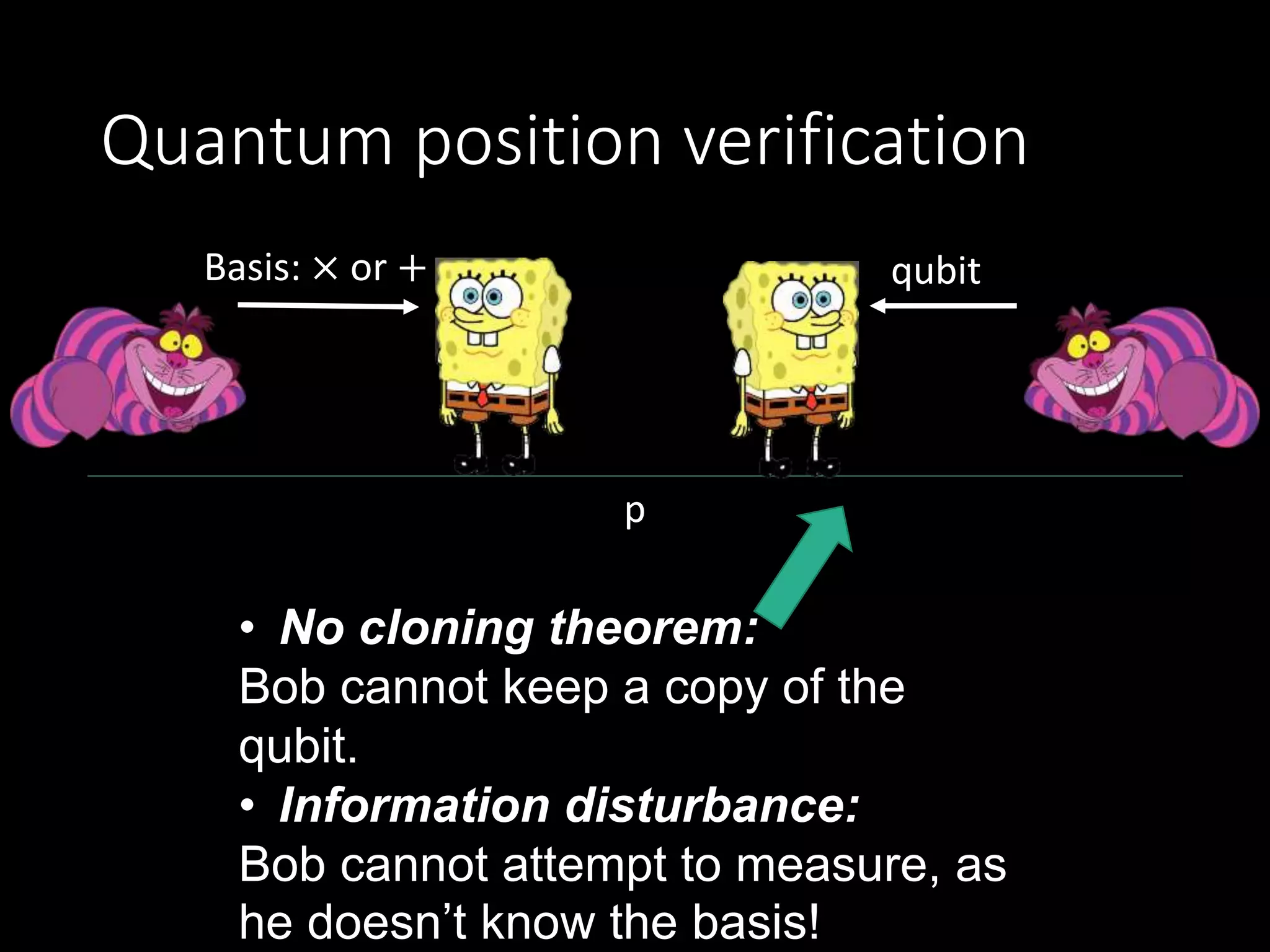
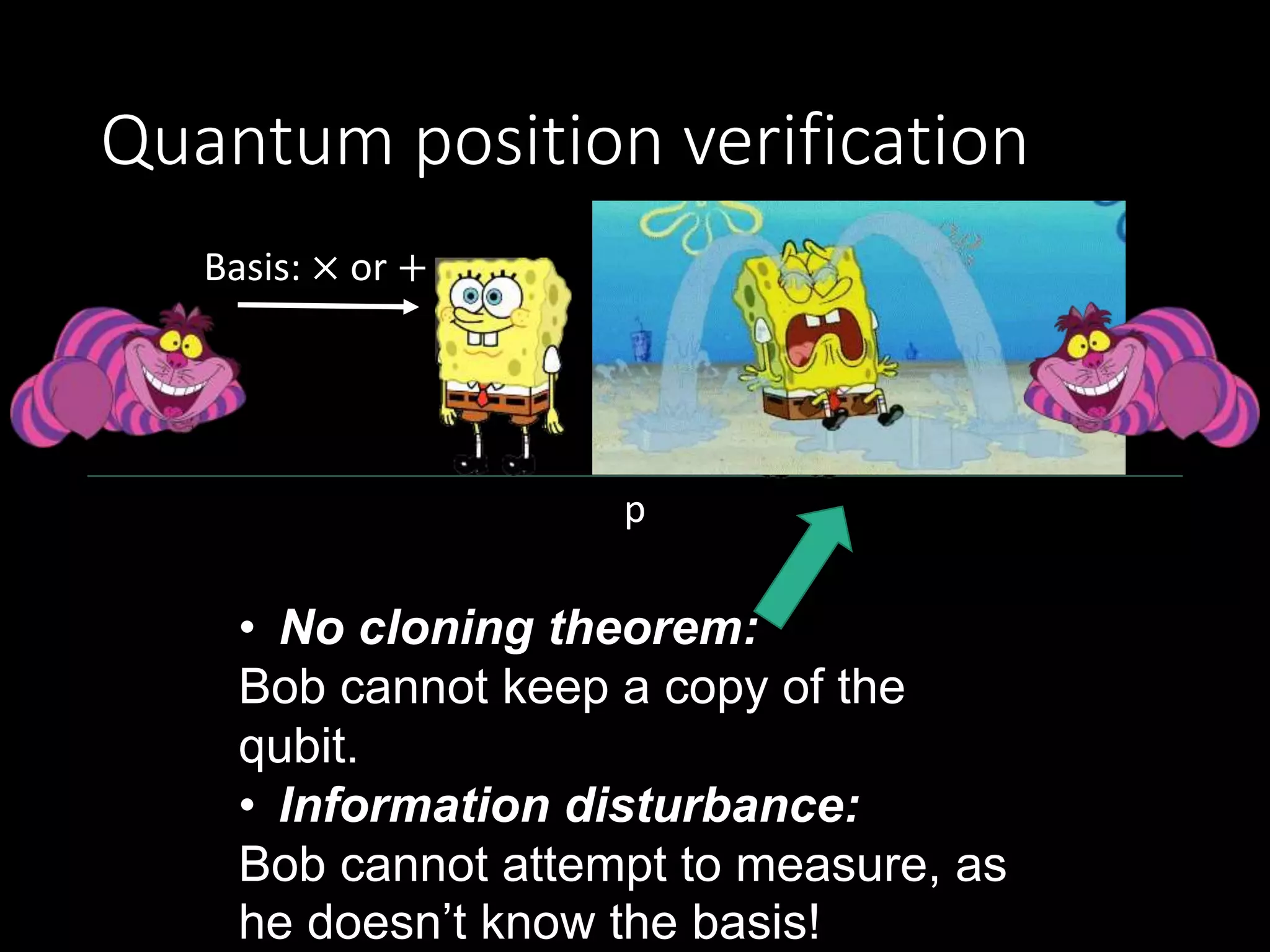
Describes aspects of quantum key distribution, emphasizing the no-cloning theorem and secure communication.
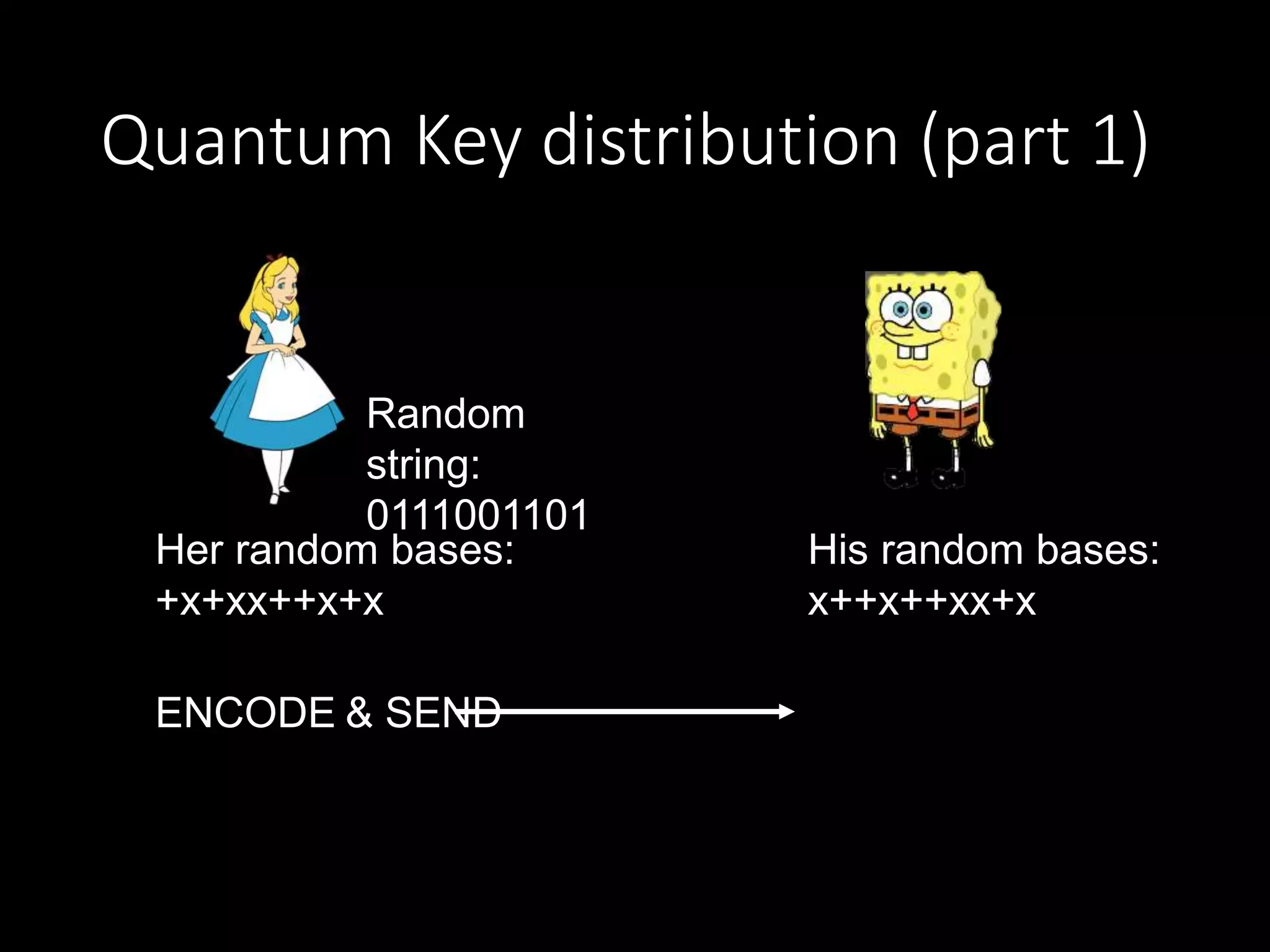
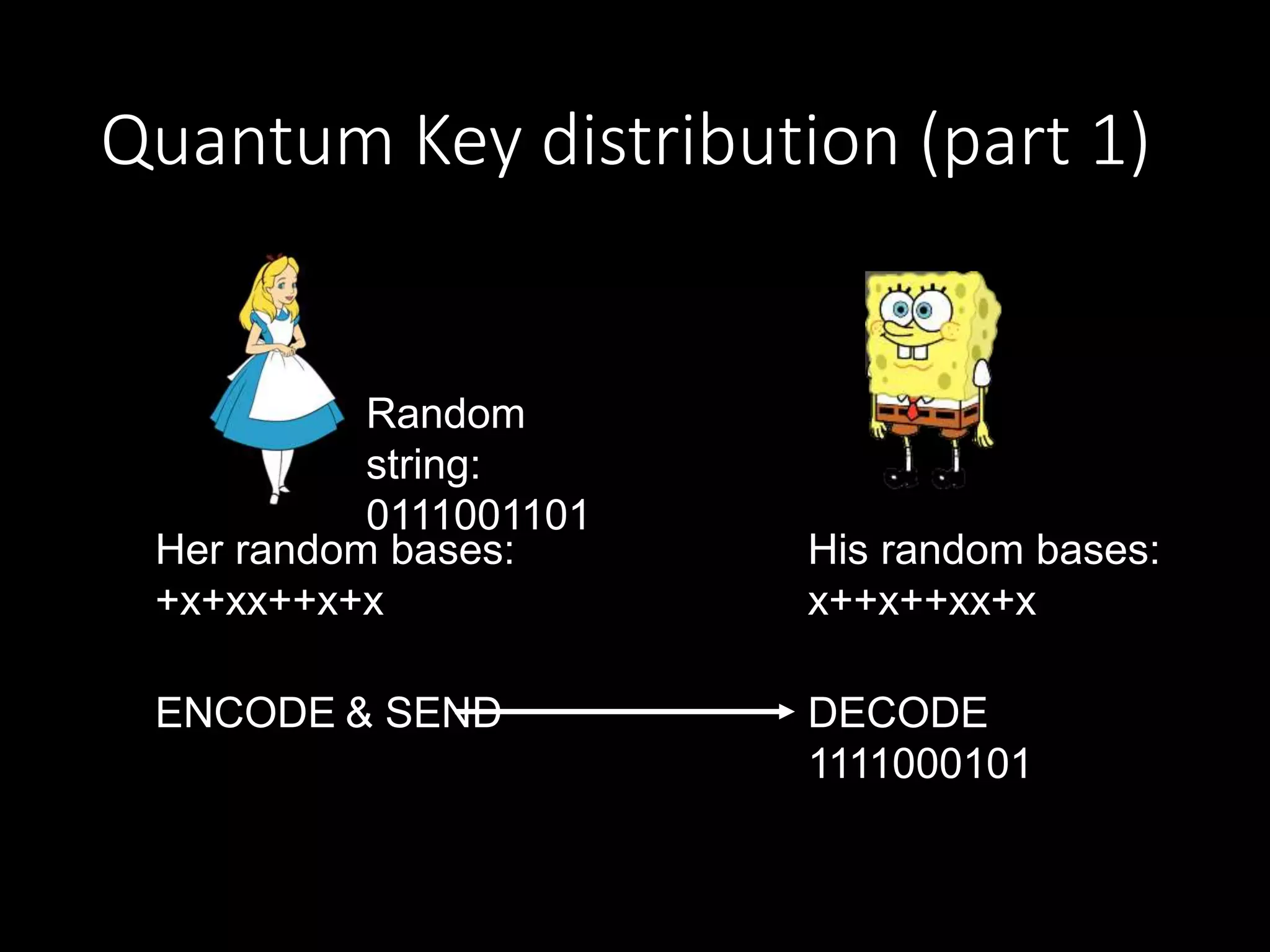
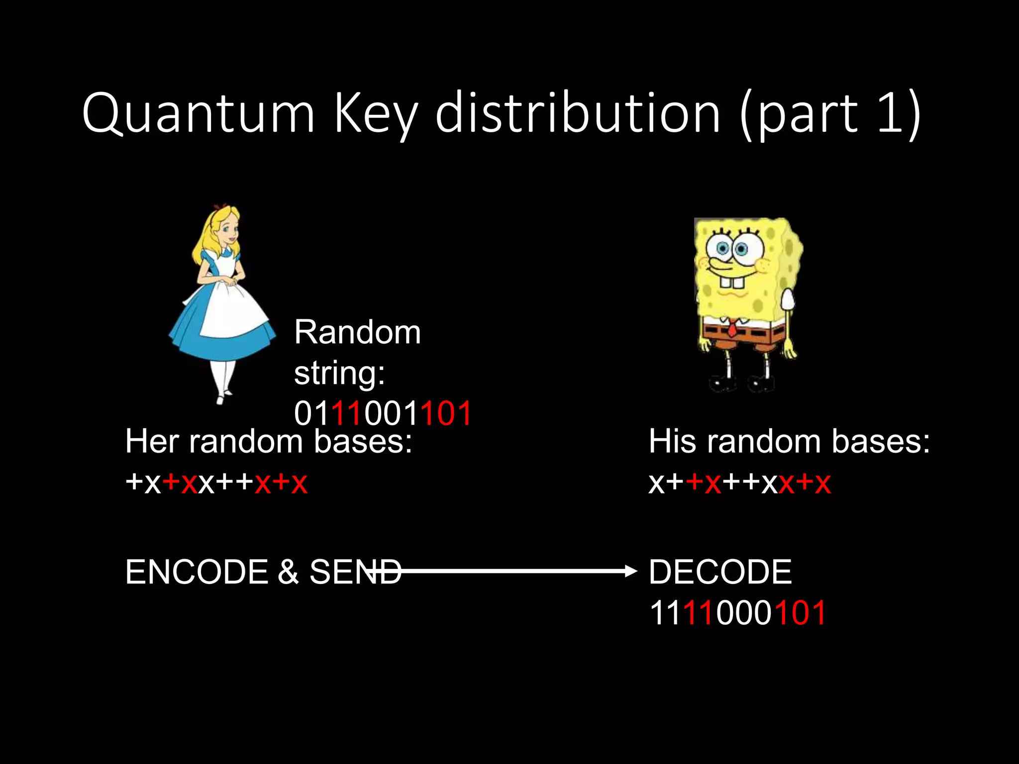
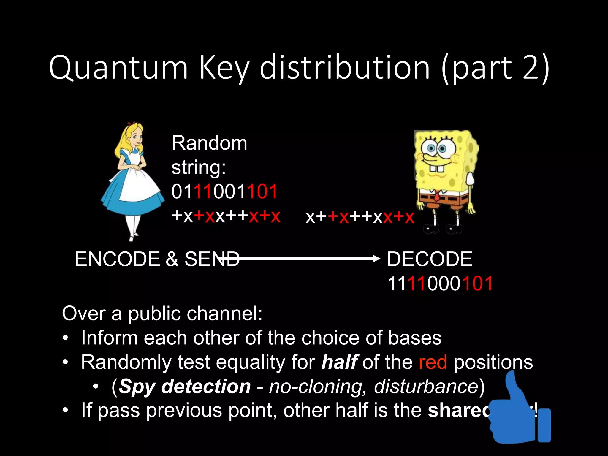
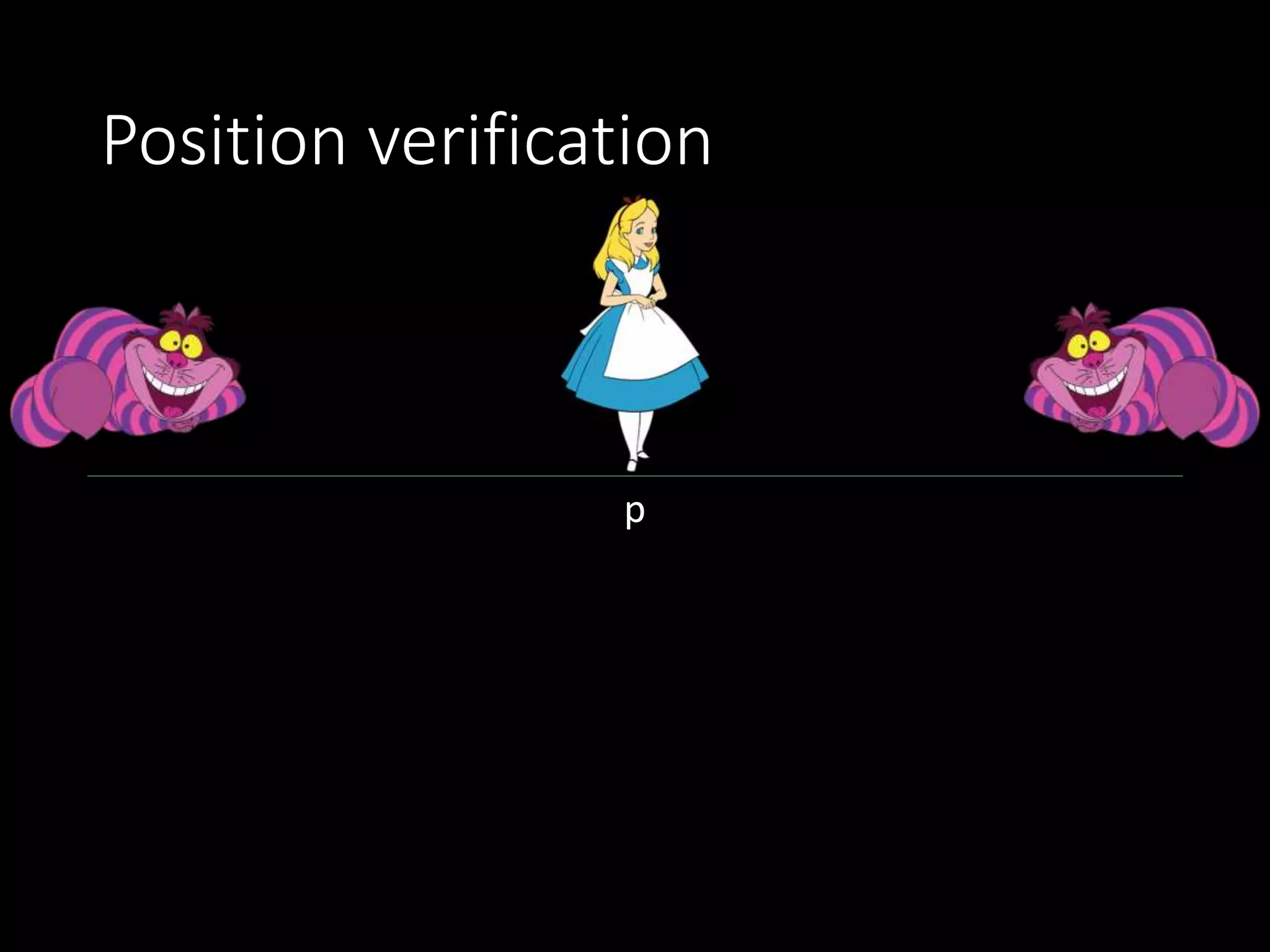
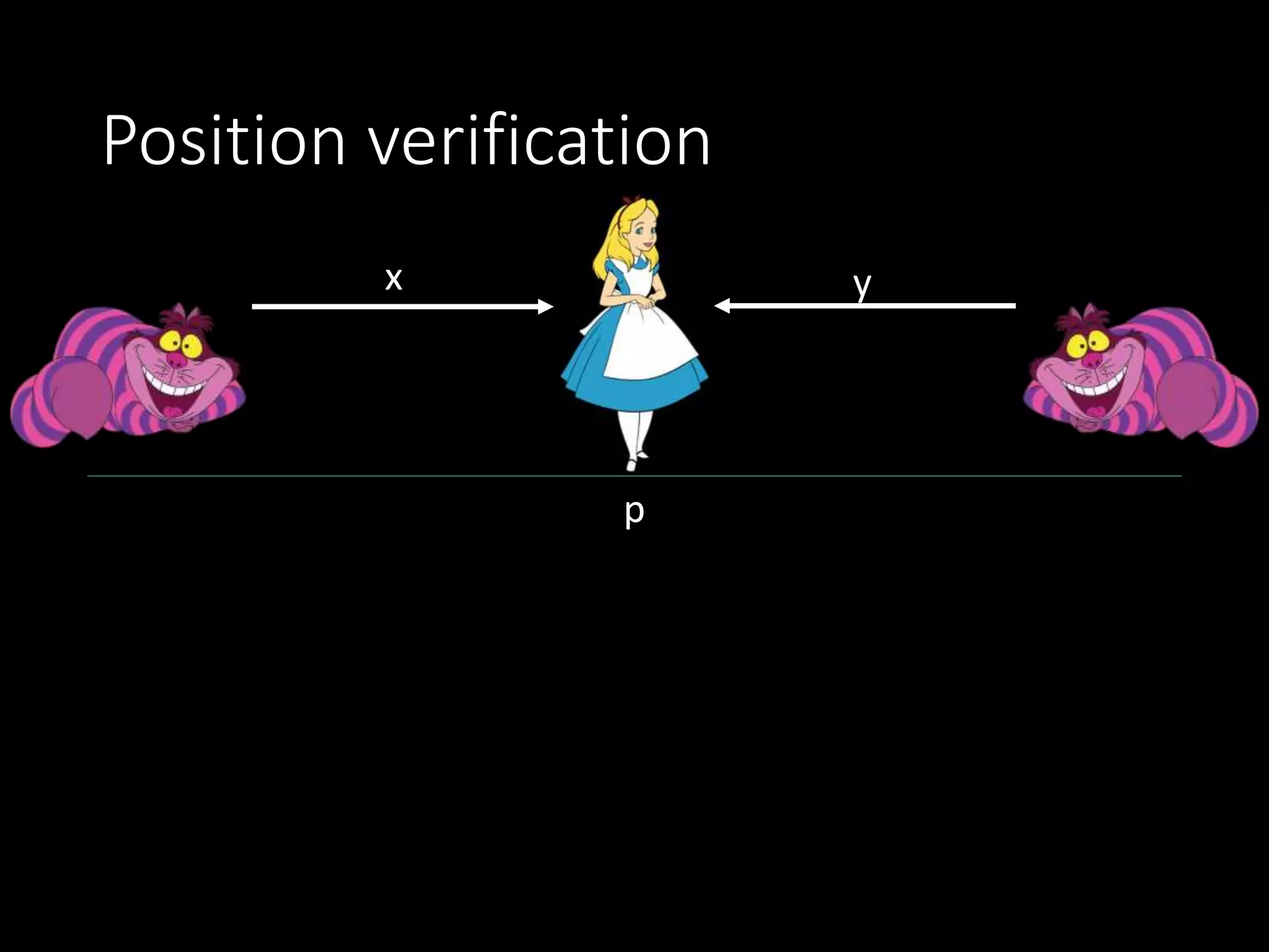
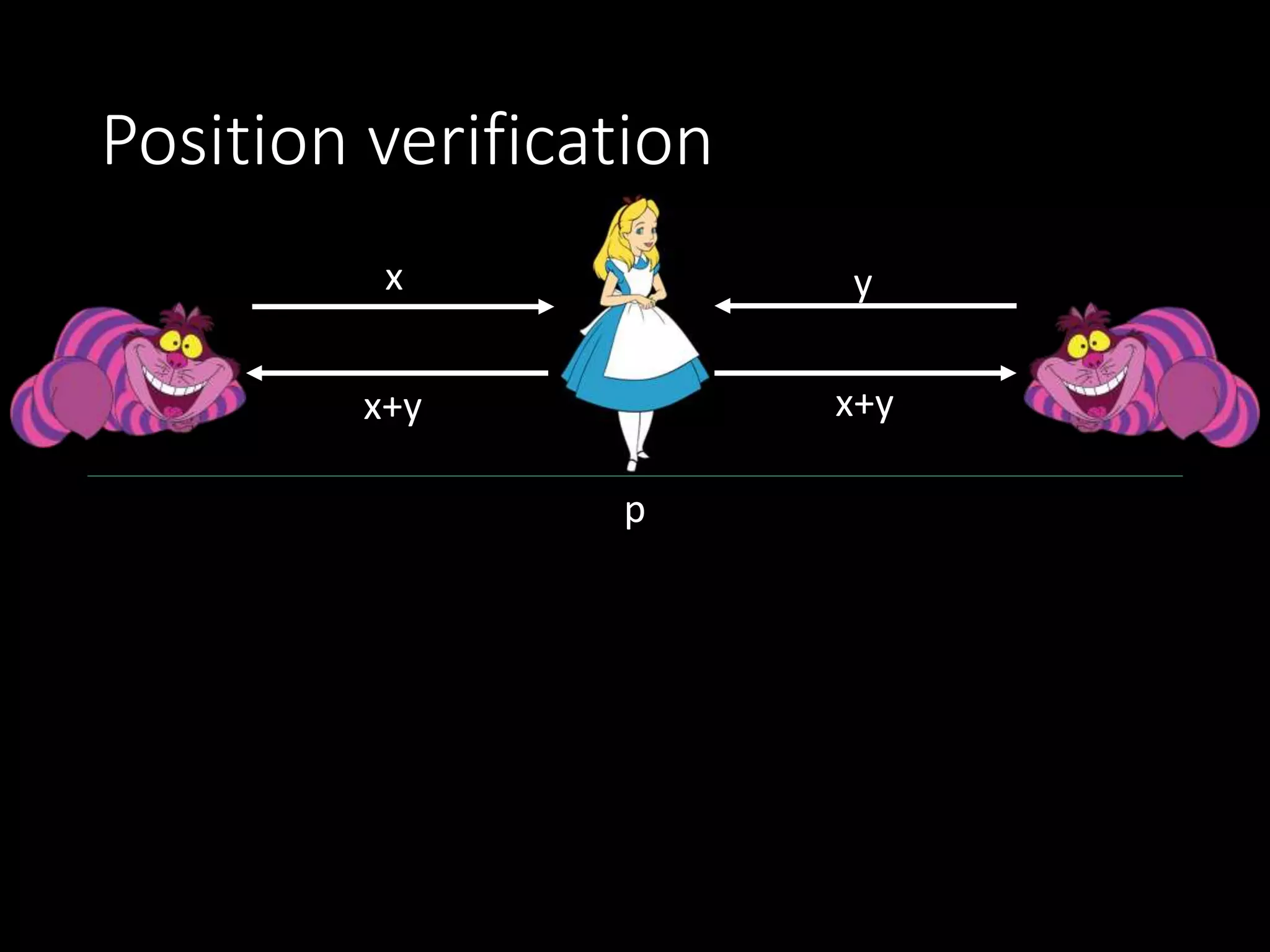
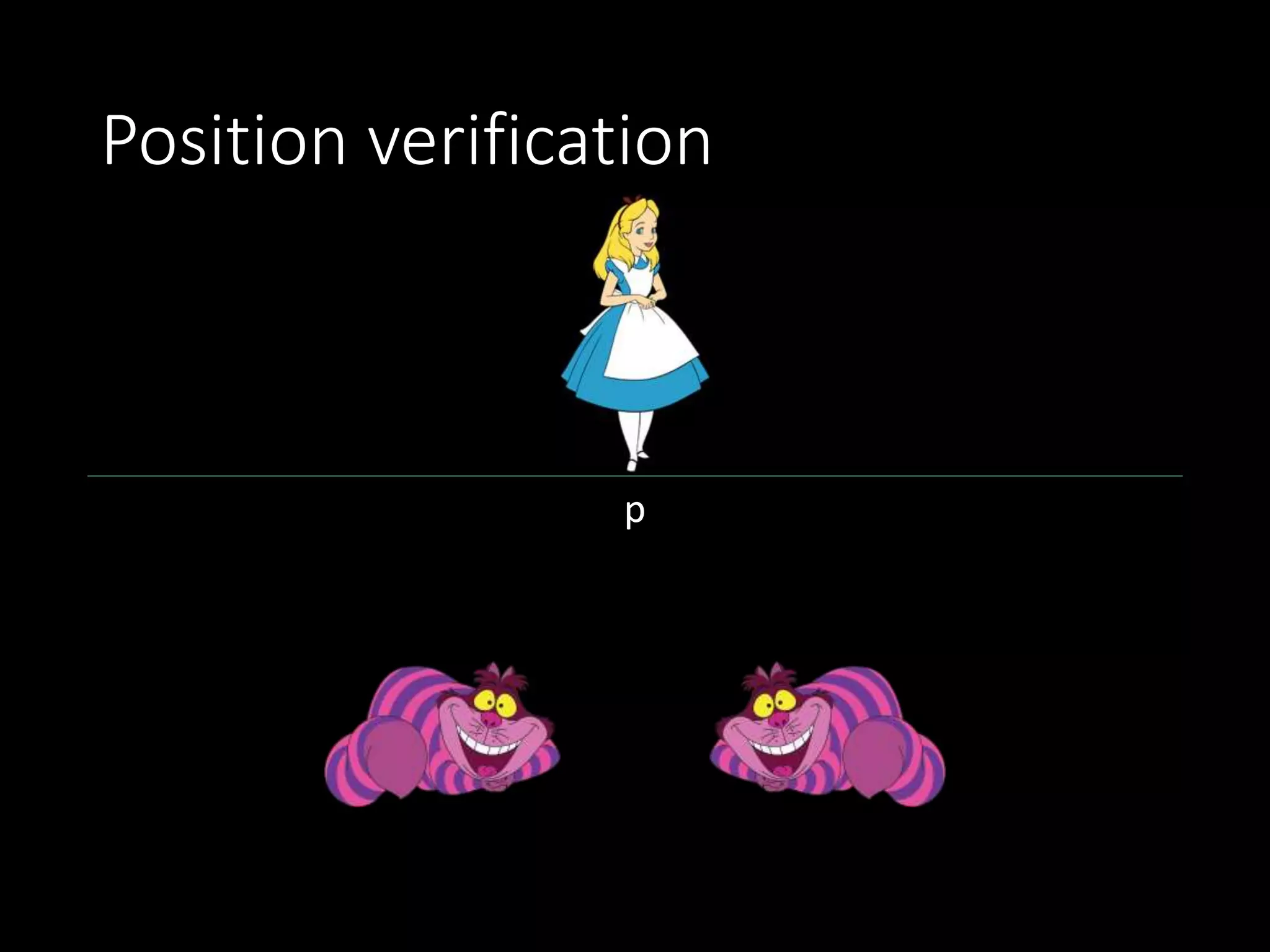
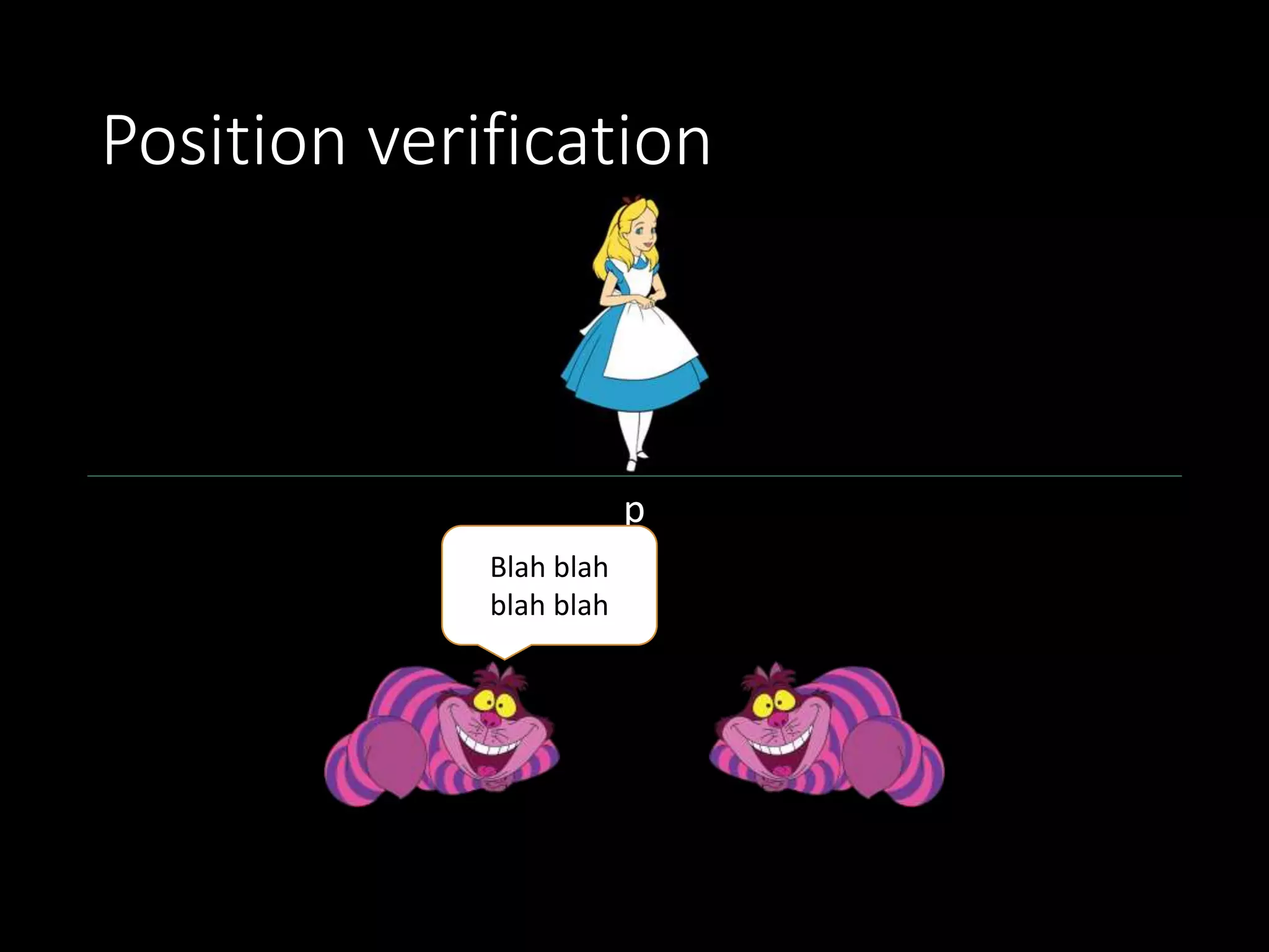
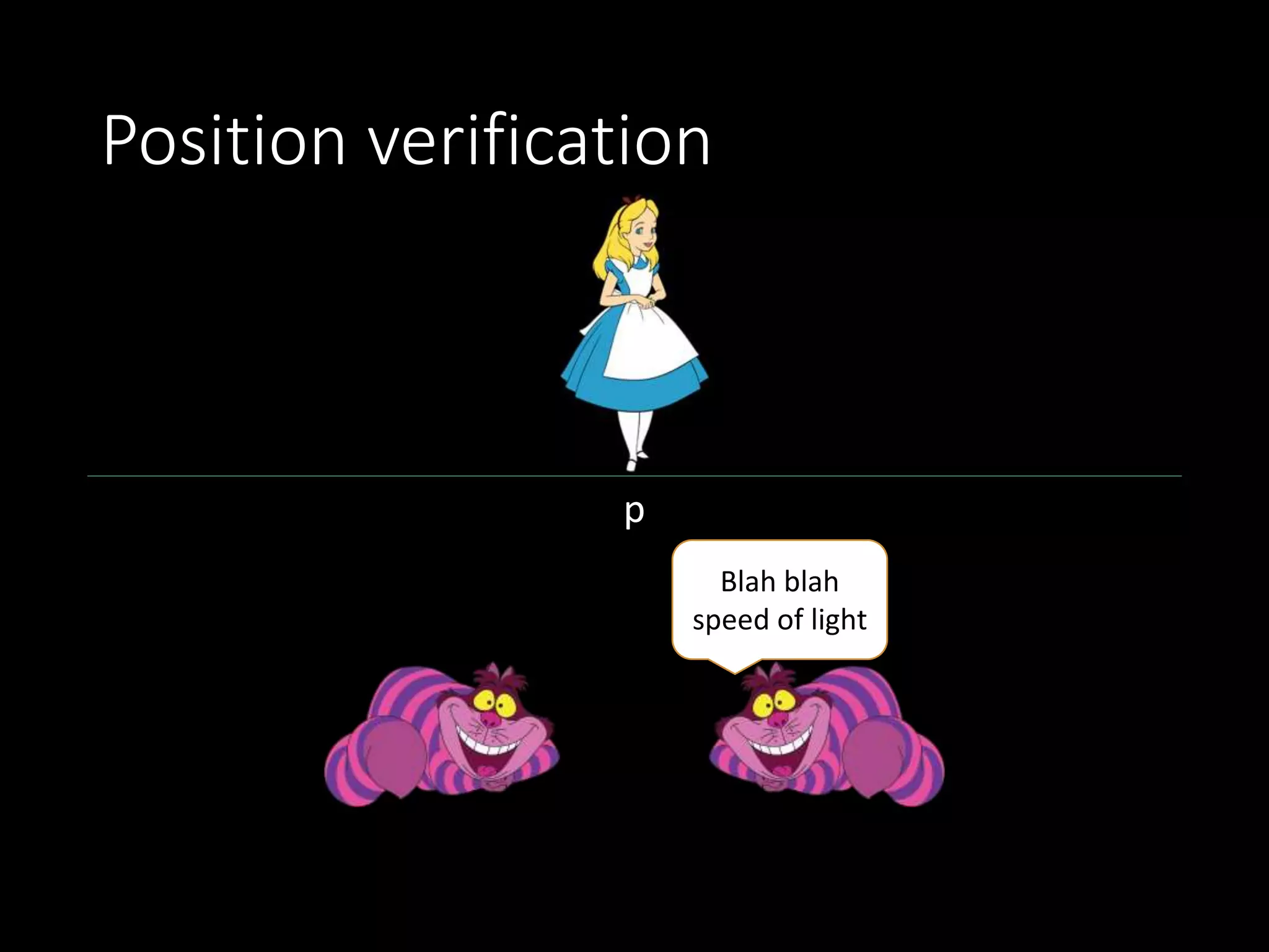
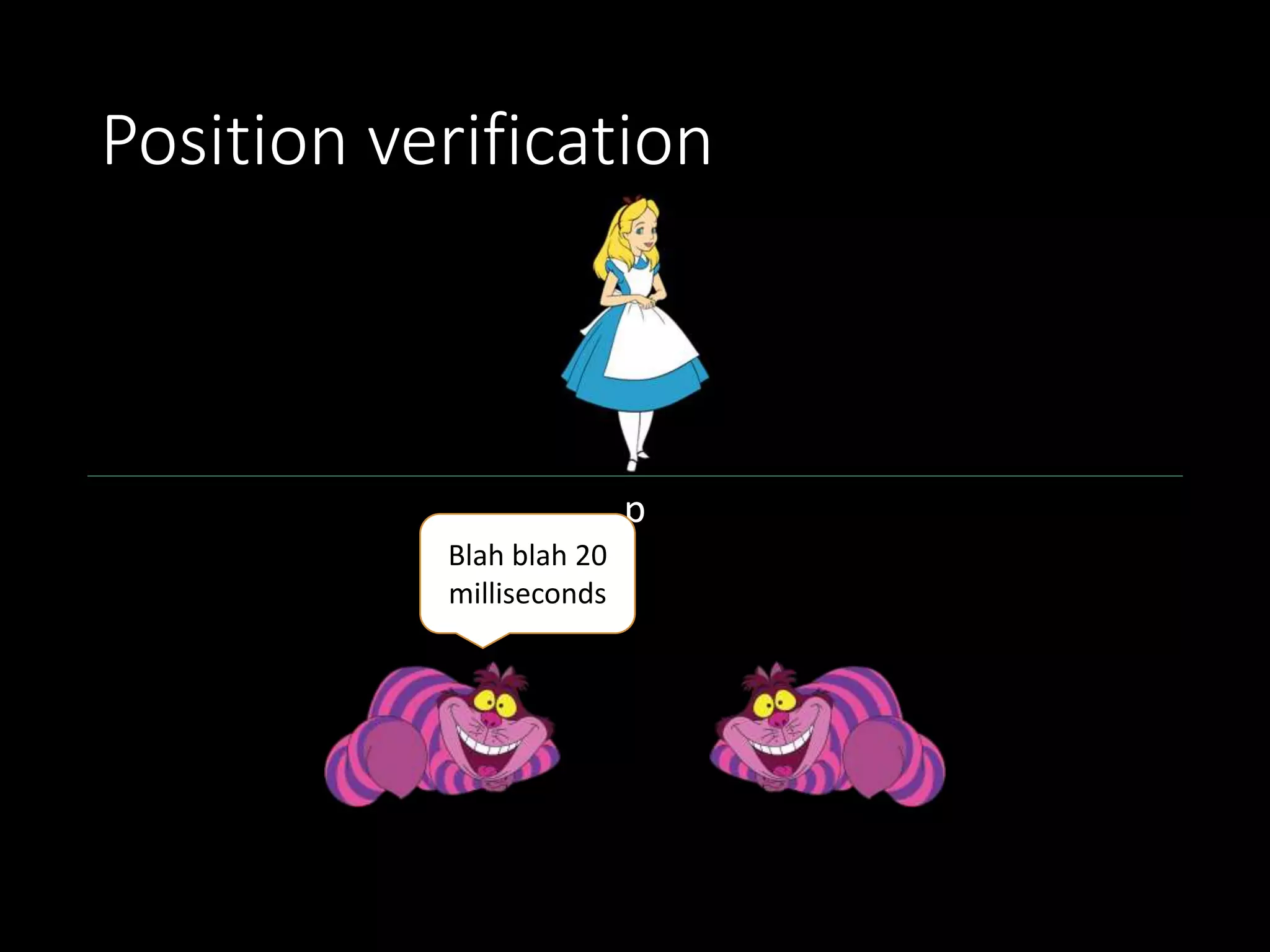
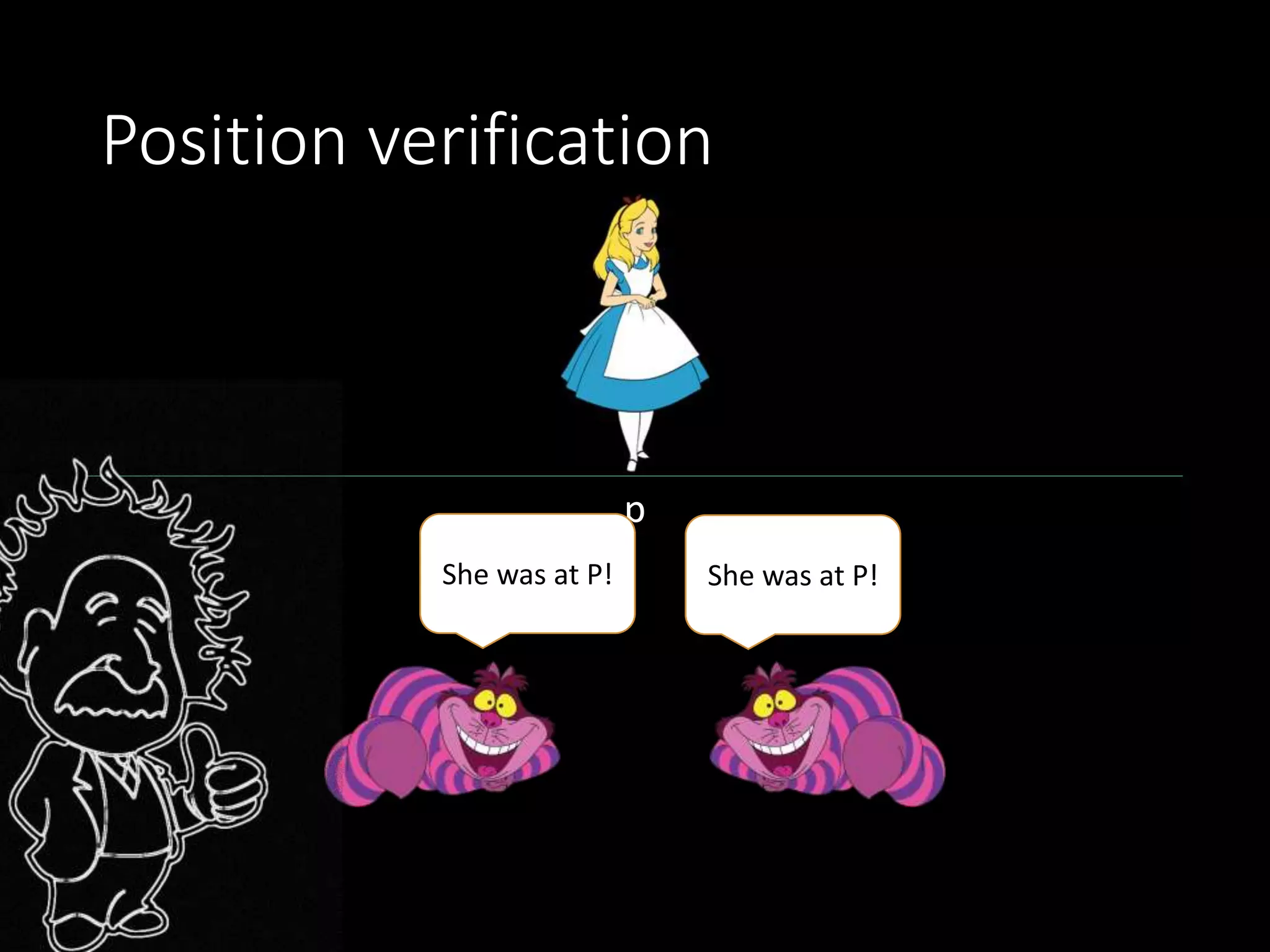
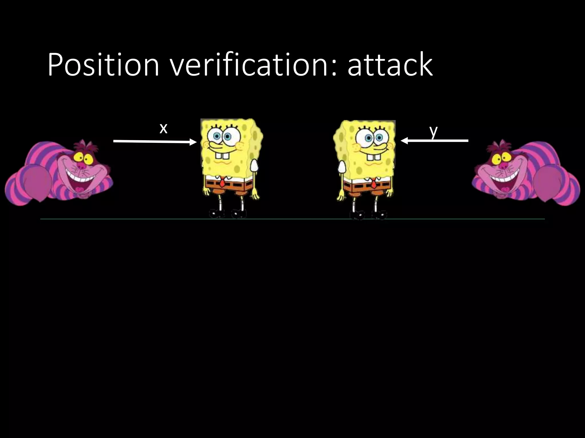
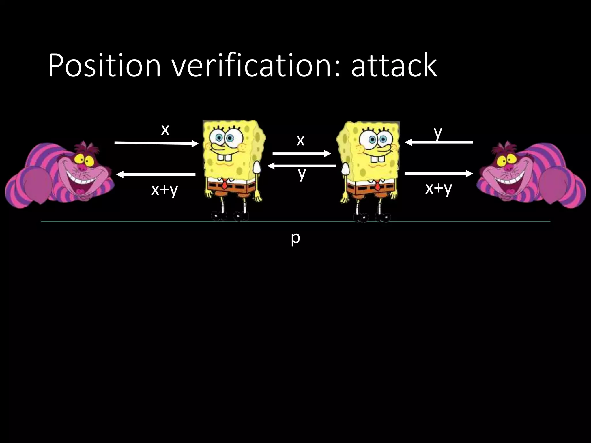
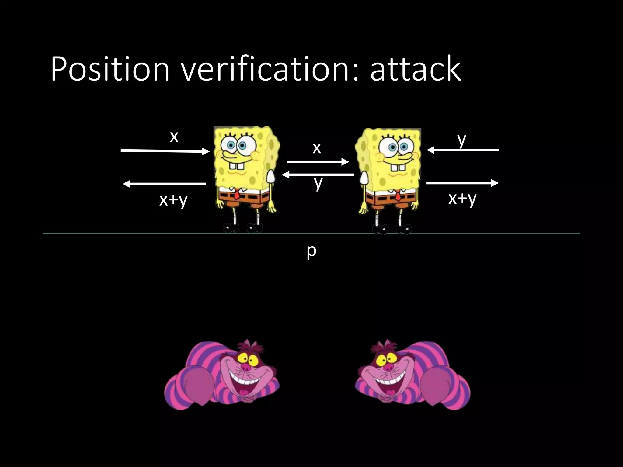
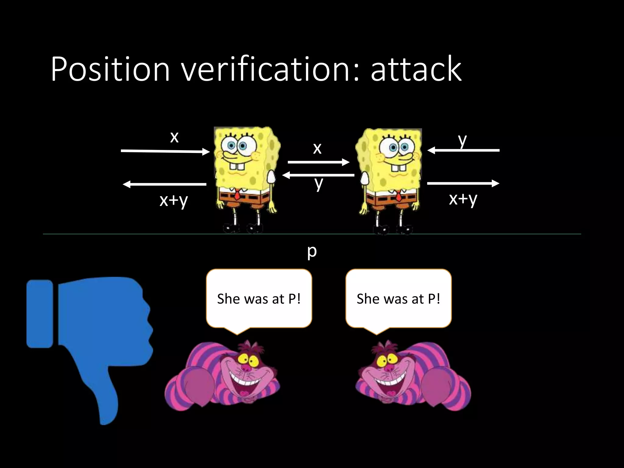
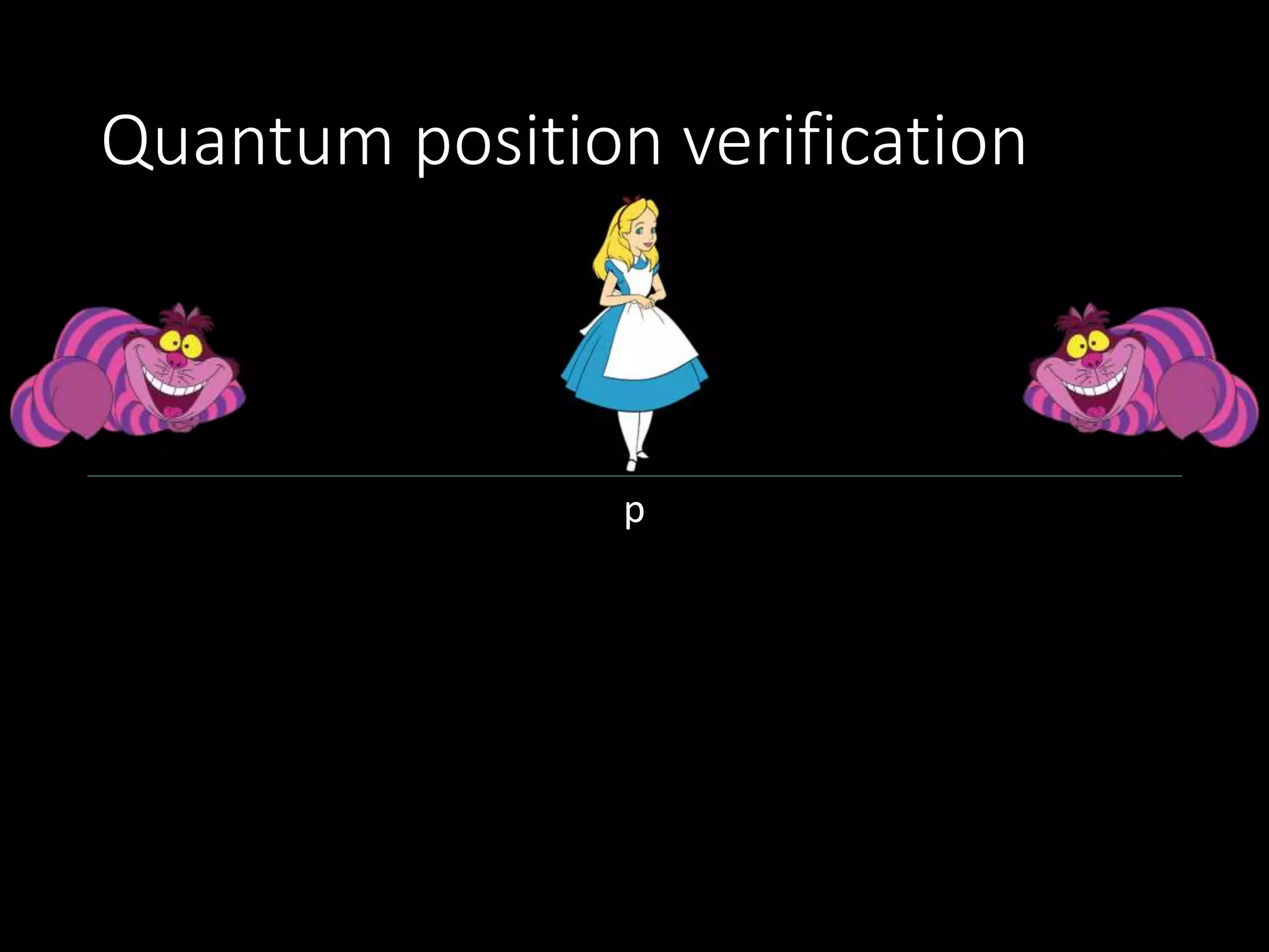
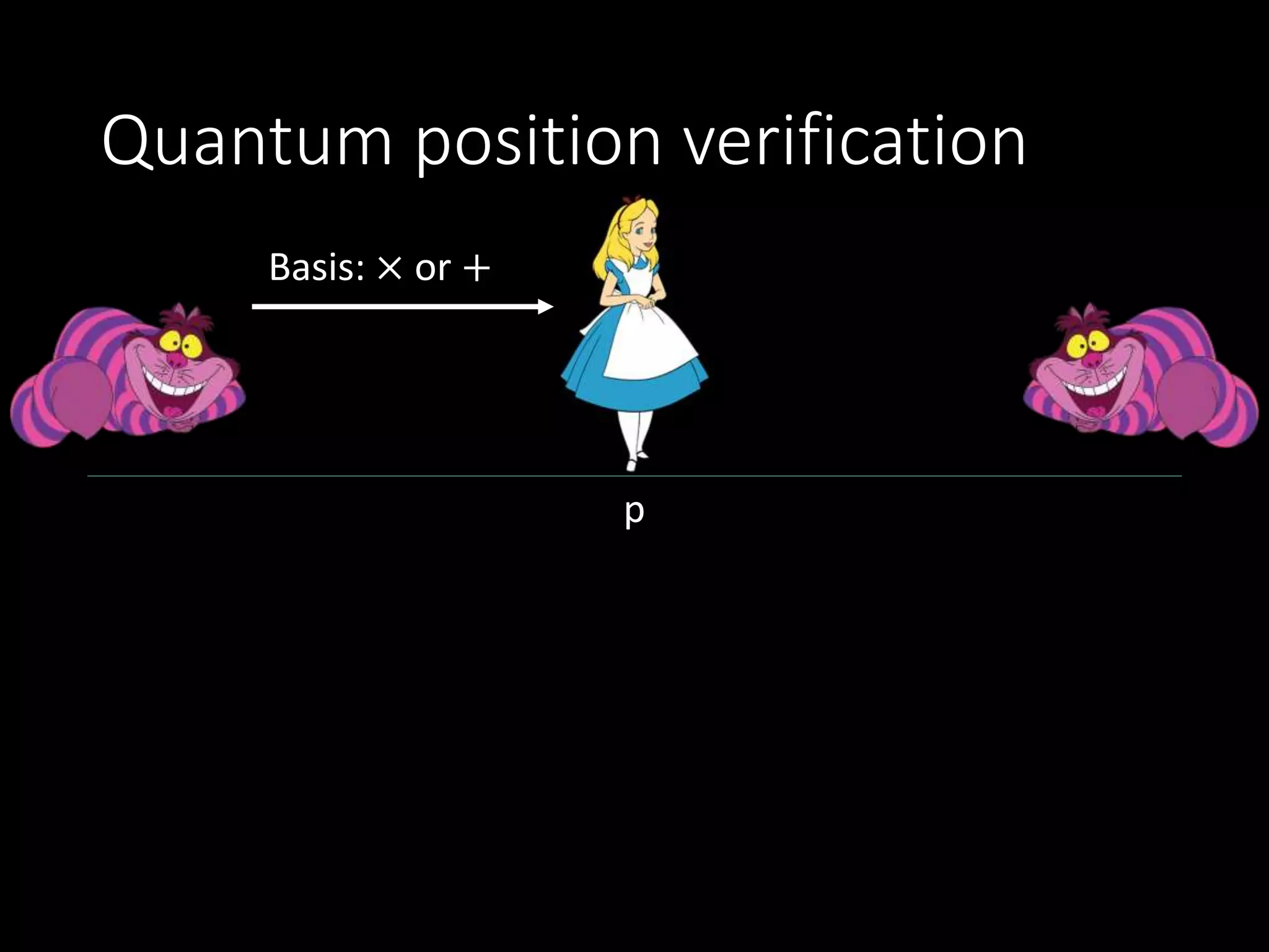
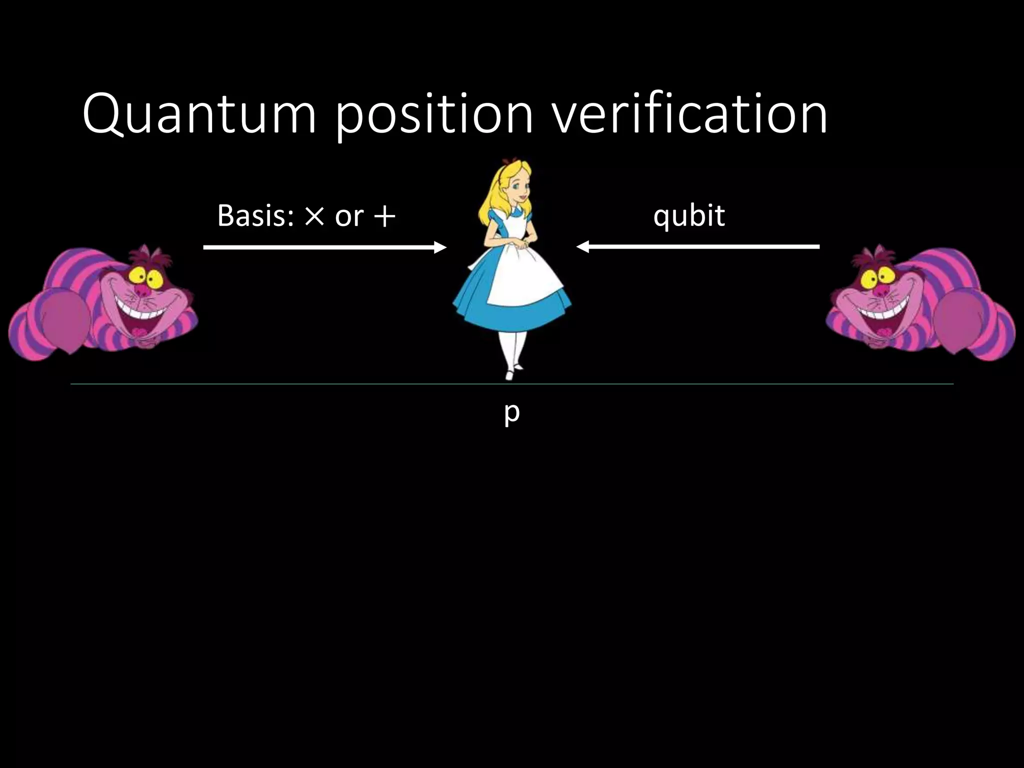
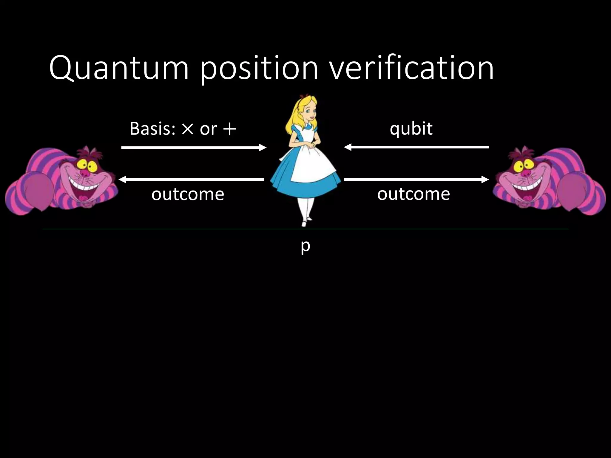
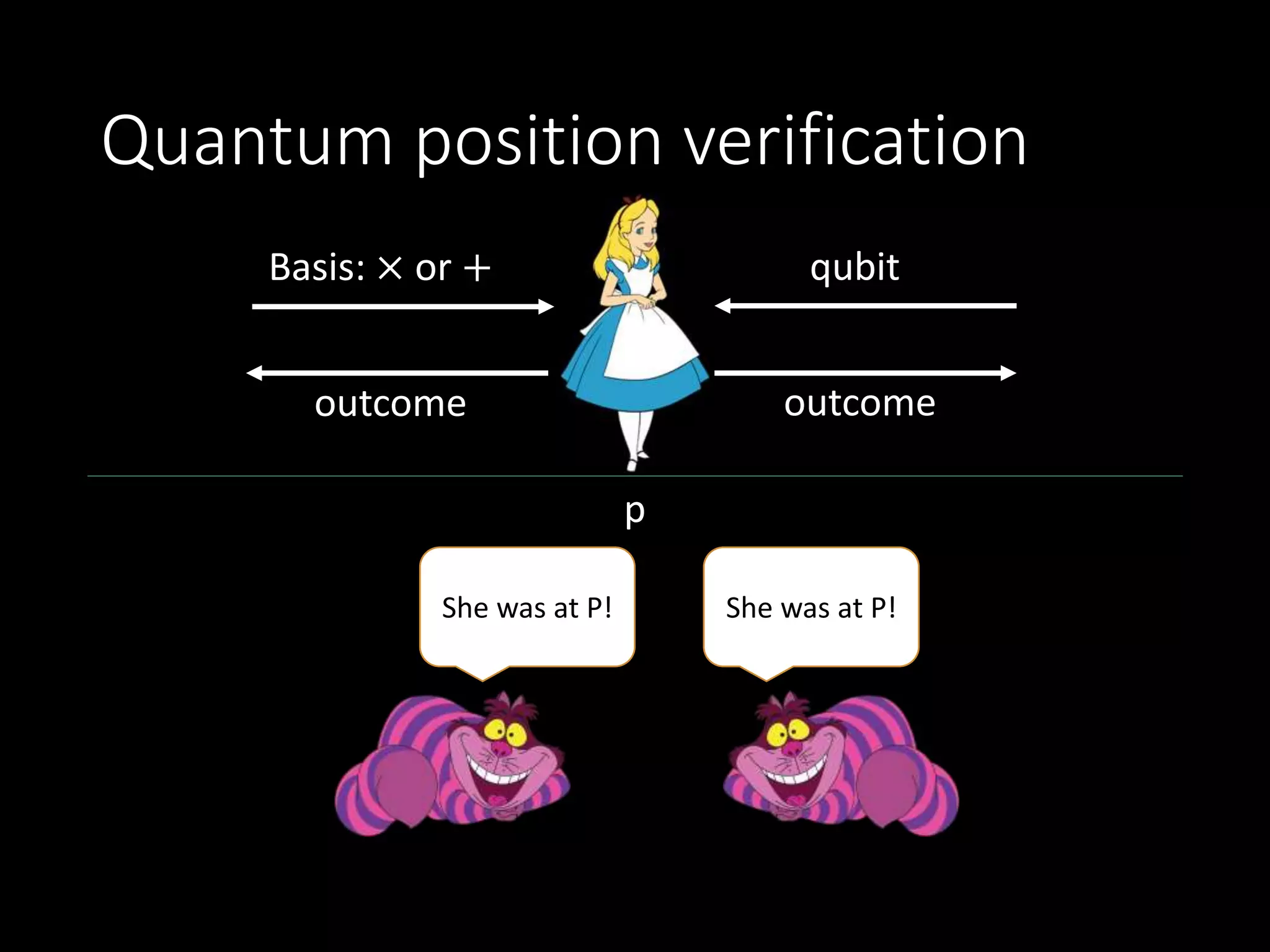
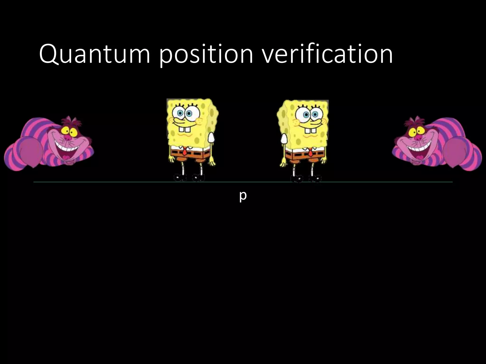
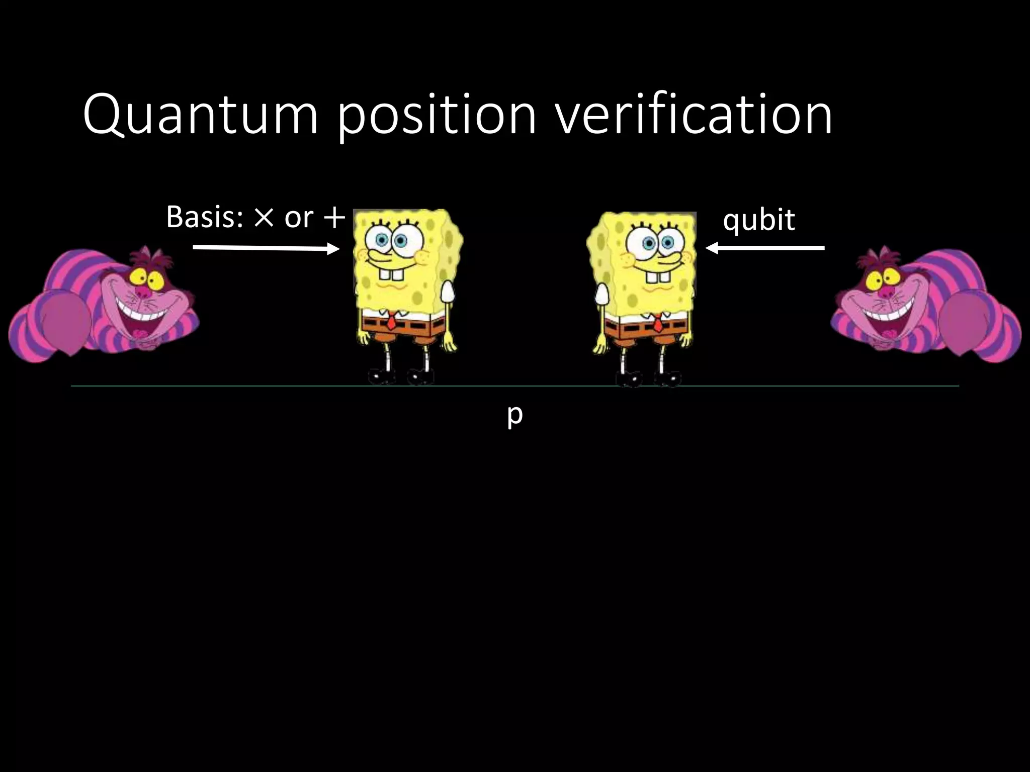
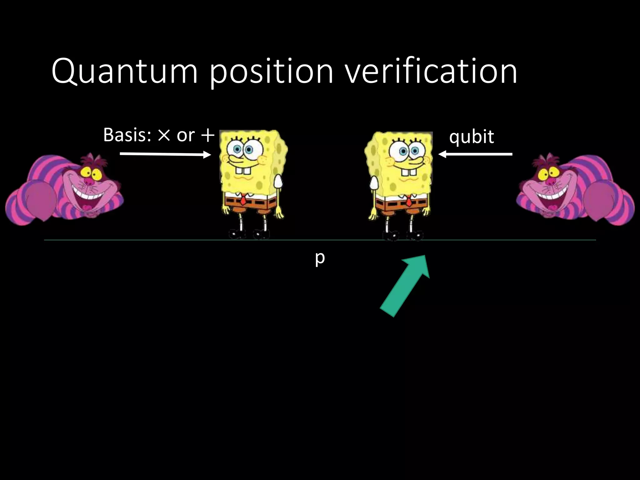
Details the steps in actual quantum key distribution including encoding, sending, and decoding messages.Discusses quantum position verification protocols, including security aspects like no-cloning and information disturbance.
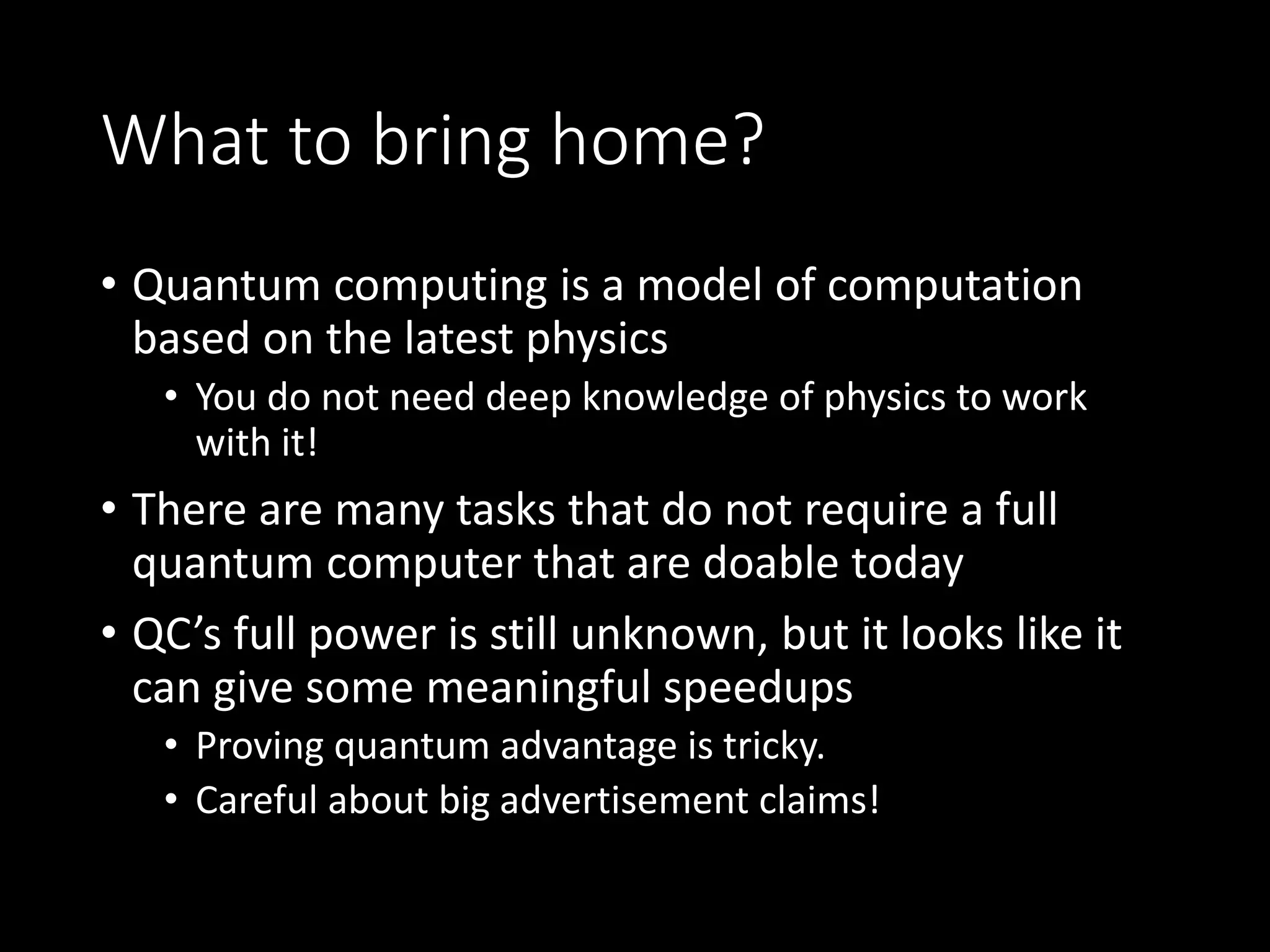
Summarizes the significance of quantum computing, addressing common questions about its reality and potential.