Download as PDF, PPTX
![The most important property of this [IHLS] space is a “well-
behaved” saturation coordinate which, in contrast to commonly
used ones, always has a small numerical value for near-
achromatic colours, and is completely independent of the
brightness function
A 3D-polar Coordinate Colour Representation Suitable for
Image, Analysis Allan Hanbury and Jean Serra
MATLAB routines implementing the RGB-to-IHLS and IHLS-to-RGB are
available at http://www.prip.tuwien.ac.at/˜hanbury.
R routines implementing the RGB-to-IHLS and IHLS-to-RGB are
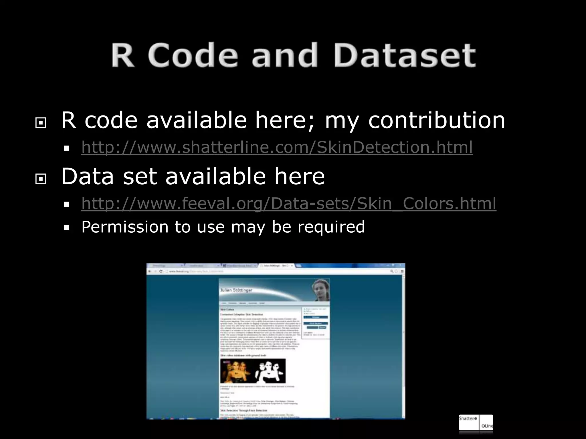
available at http://www.shatterline.com/SkinDetection.html](https://image.slidesharecdn.com/arandomforestapproachtoskindetectionwithr-13540352993178-phpapp01-121127105541-phpapp01/75/A-Random-Forest-Approach-To-Skin-Detection-With-R-9-2048.jpg)
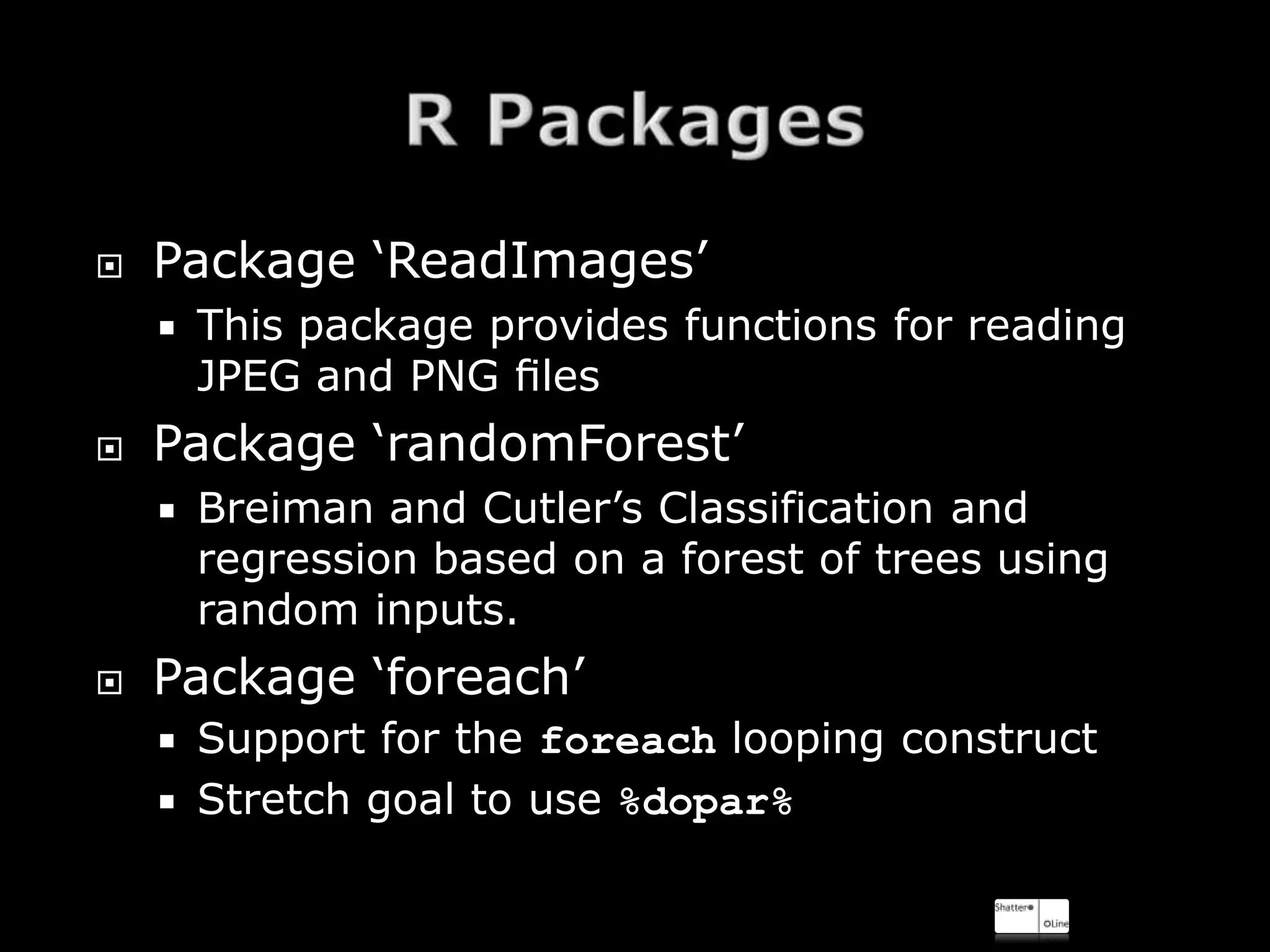
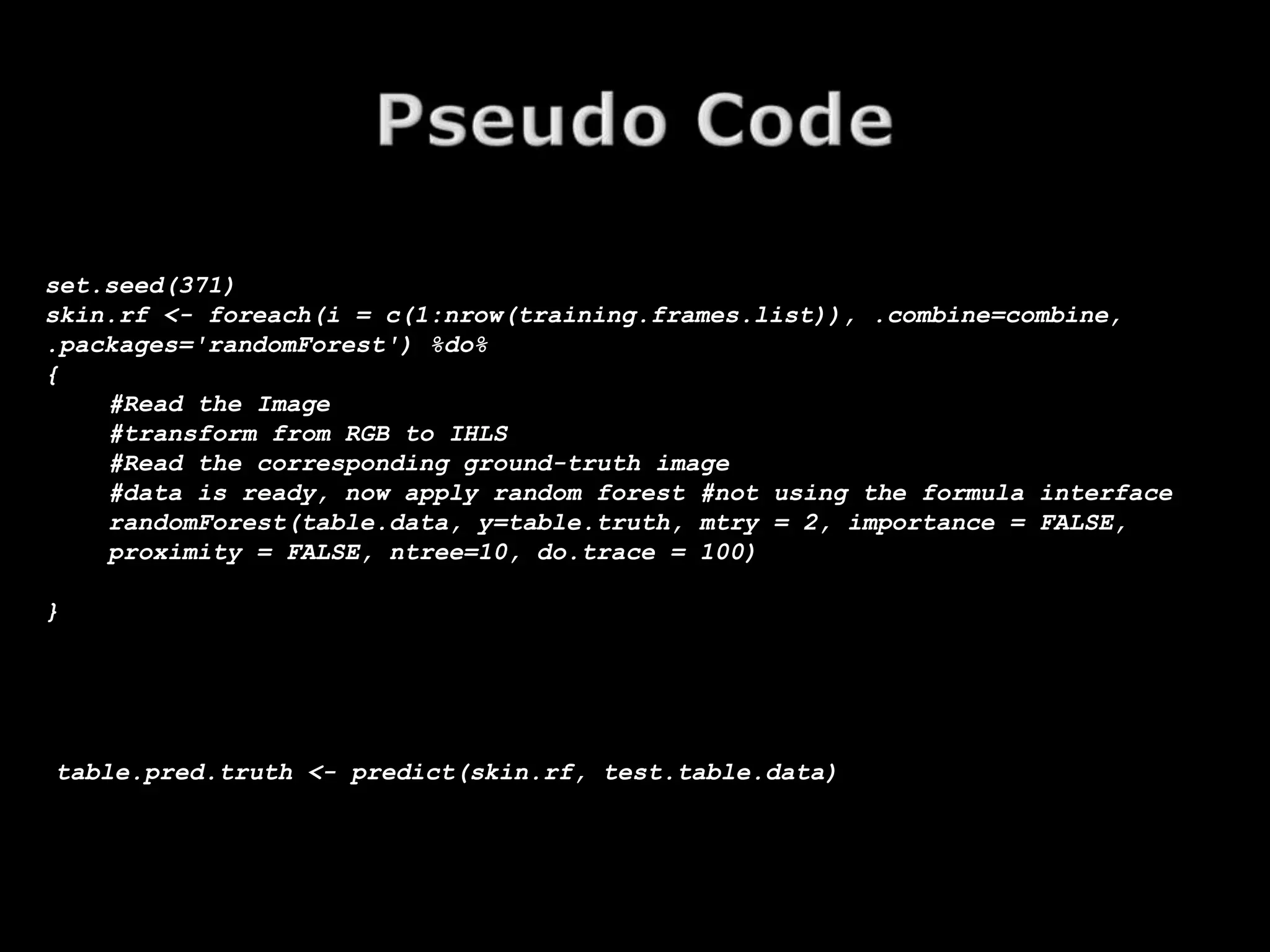
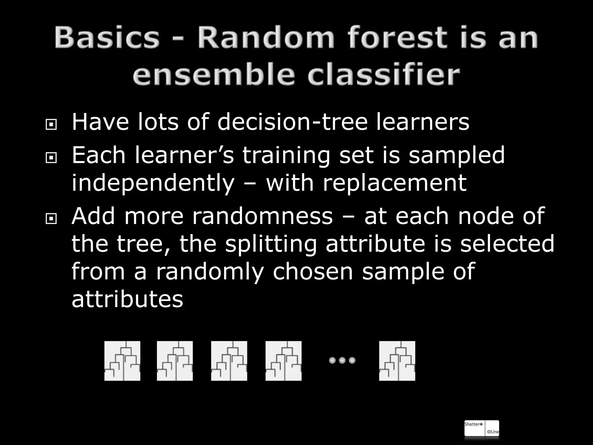
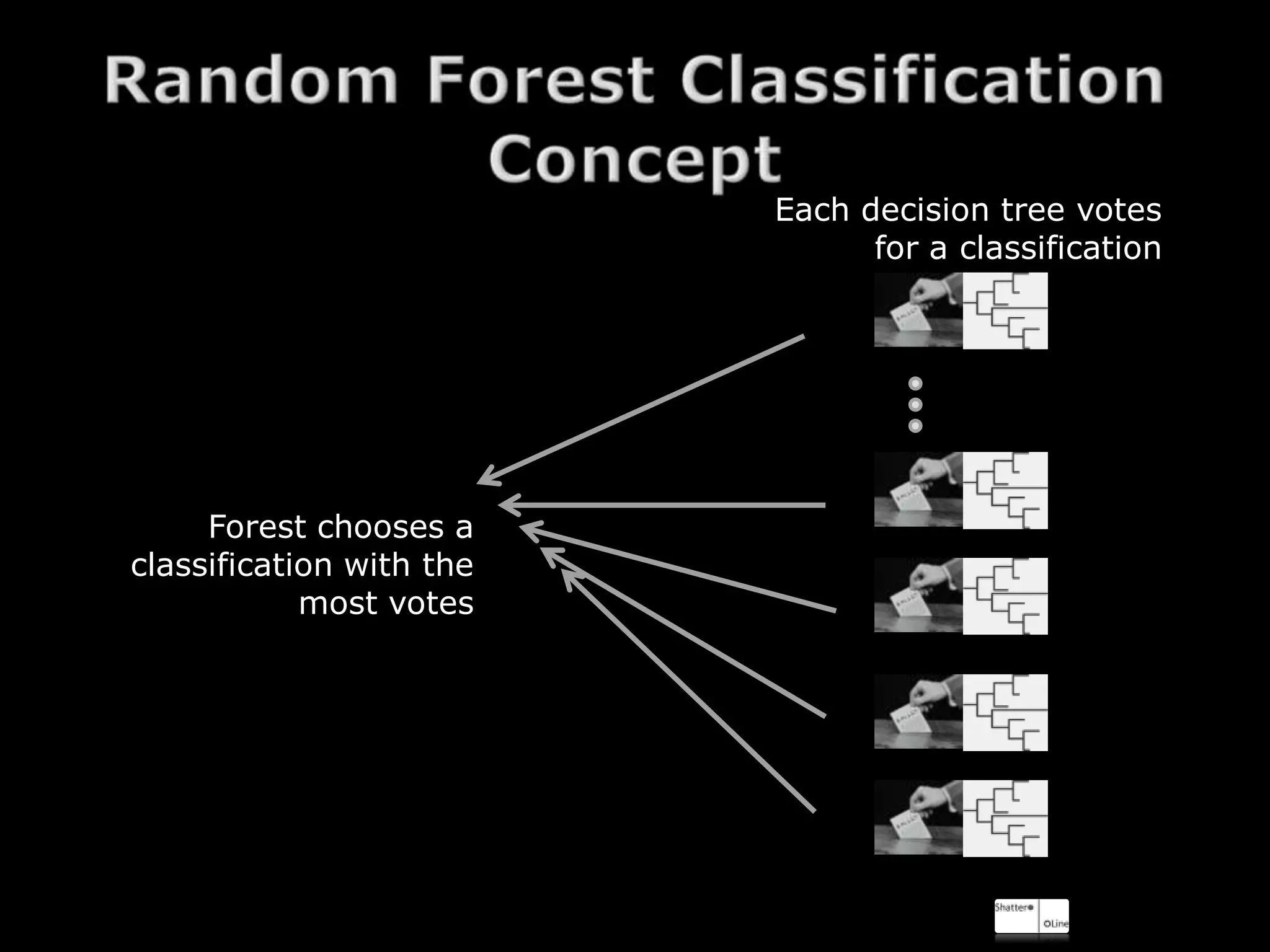
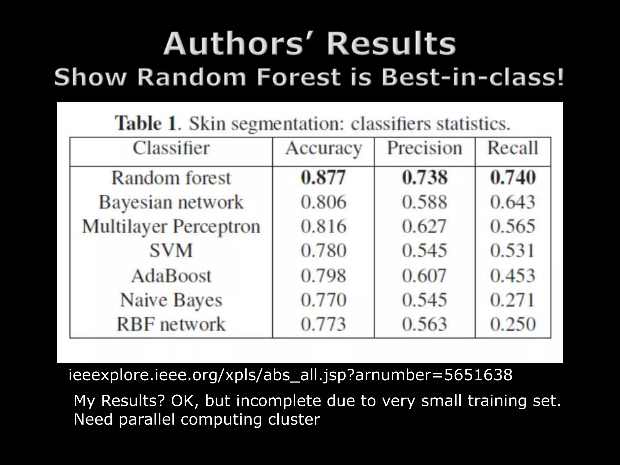

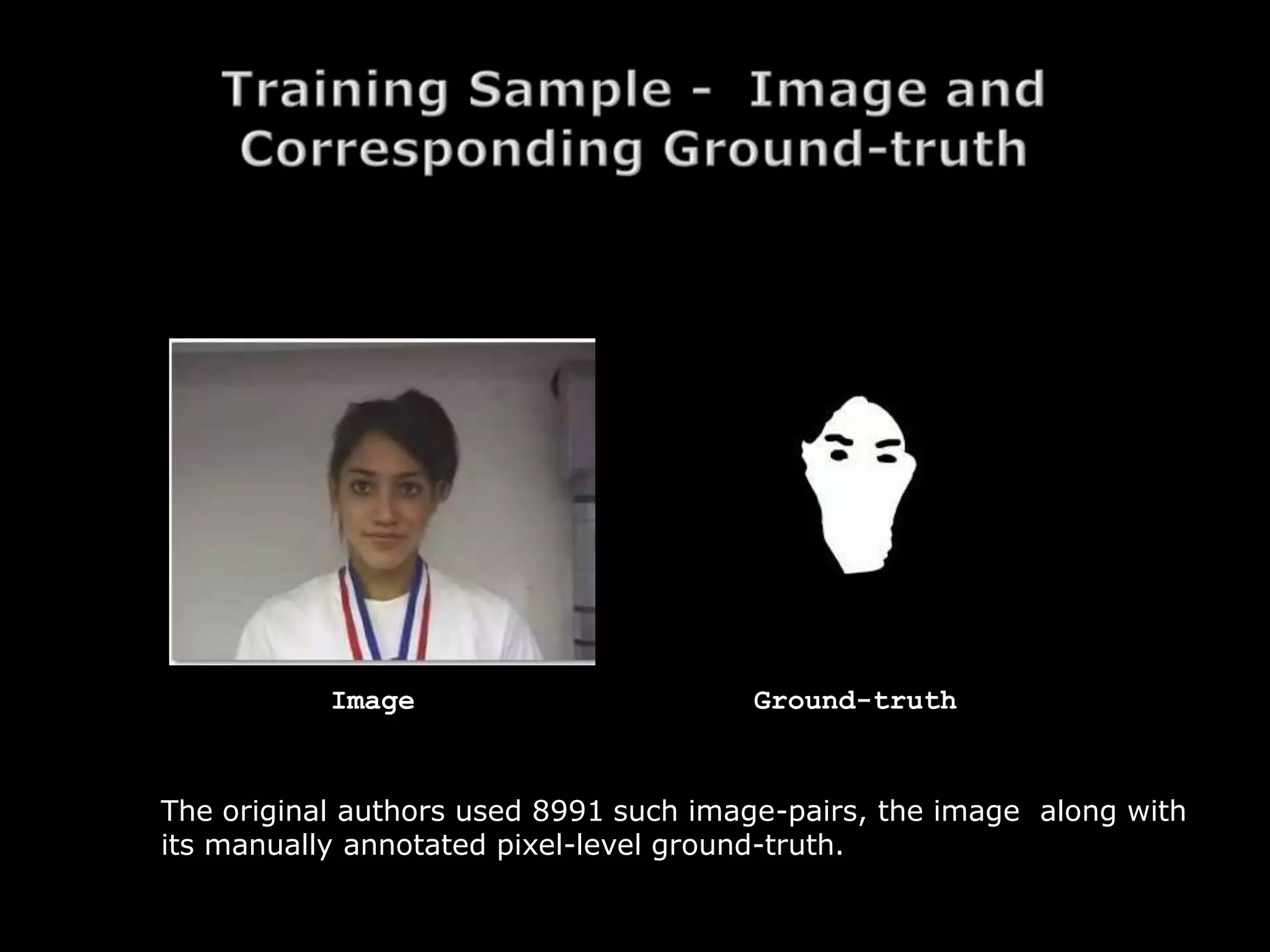
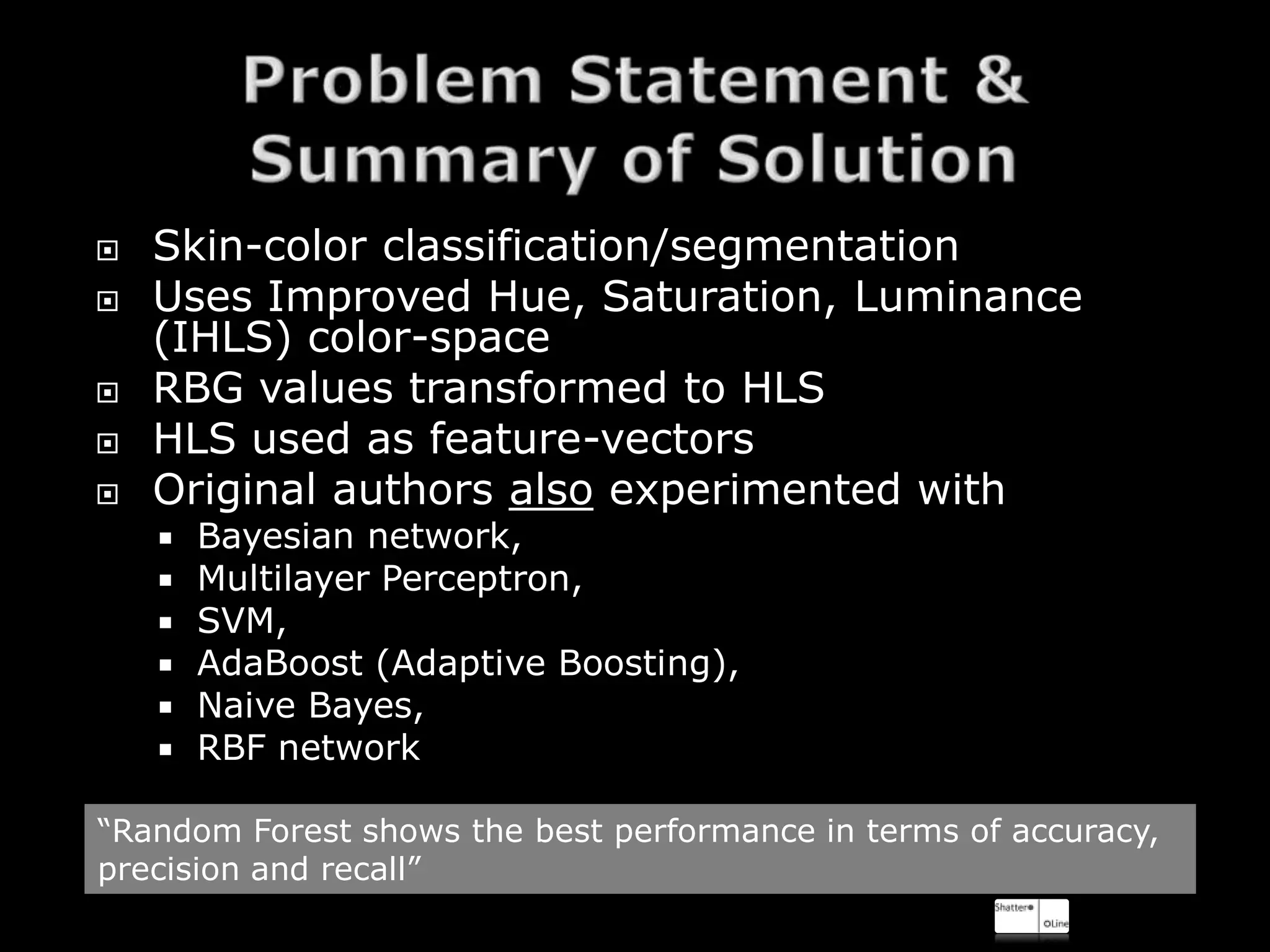
The document discusses using random forests for skin detection from images. It provides an overview of the scheme, which uses improved Hue, Saturation, Luminance (IHLS) color space and transforms RGB values to IHLS features. Random forests showed the best performance compared to other models. The document references code and datasets, provides details on implementing random forests in R, and states results were incomplete due to a small training set and need for parallel computing. It concludes with time for questions.