Download as PDF, PPTX

![Hidden Markov Random Field
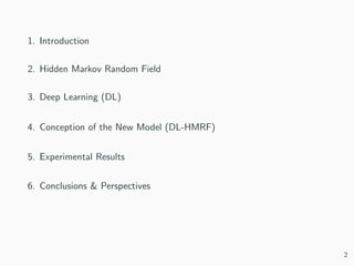
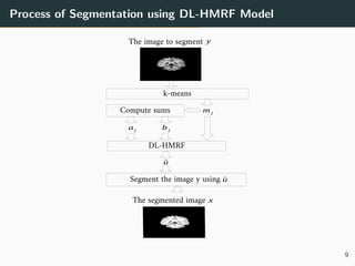
The image to segment y = {ys}s∈S
into K classes is a realization of Y
• Y = {Ys}s∈S is a family of random
variables
• ys ∈ [0 . . . 255]
The segmented image into K classes
x = {xs}s∈S is realization of X
• X = {Xs}s∈S is a family of random
variables
• xs ∈ {1, . . . , K}
An example of segmentation into
K = 4 classes
x∗
= argx∈Ω max {P[X = x | Y = y]}
5](https://image.slidesharecdn.com/aiccsa20201-201130113451/85/3D-Brain-Image-Segmentation-Model-using-Deep-Learning-and-Hidden-Markov-Random-Fields-7-320.jpg)
![Hidden Markov Random Field
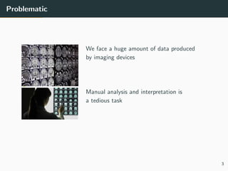
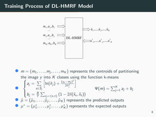
• This elegant model leads to the optimization of an energy function
Ψ(x, y) = s∈S ln(σxs
) +
(ys −µxs )2
2σ2
xs
+ β
T c2={s,t} (1 − 2δ(xs, xt))
• Our way to look for the minimization of Ψ(x, y) is to look for the
minimization Ψ(µ), µ = (µ1, . . . , µK ) where µi are means of gray
values of class i
Ψ(µ) =
K
j=1
s∈Sj
[ln(σj ) +
(ys −µj )2
2σ2
j
] + β
T
c2={s,t}
(1 − 2δ(xs, xt))
6](https://image.slidesharecdn.com/aiccsa20201-201130113451/85/3D-Brain-Image-Segmentation-Model-using-Deep-Learning-and-Hidden-Markov-Random-Fields-8-320.jpg)
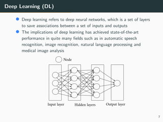
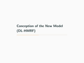
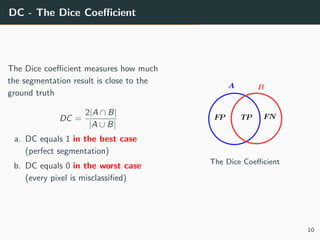
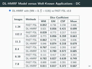
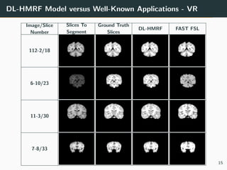


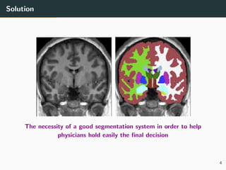
The document presents a 3D brain image segmentation model using deep learning and hidden Markov random fields (HM_RF), developed to aid physicians in analyzing imaging data. The study includes details on the model's conception, experimental results, and a comparison with existing methods, showing promising performance, particularly in segmentation quality. However, the training time for the model remains high, suggesting the potential use of Kubernetes clusters to optimize this aspect in the future.


![[PR12] PR-036 Learning to Remember Rare Events](https://cdn.slidesharecdn.com/ss_thumbnails/pr12pr-036learningtoremeberrareevents-170917140144-thumbnail.jpg?width=640&height=640&fit=bounds)


![Structured Forests for Fast Edge Detection [Paper Presentation]](https://cdn.slidesharecdn.com/ss_thumbnails/mc-crpresentation-141209192730-conversion-gate01-thumbnail.jpg?width=640&height=640&fit=bounds)


![Getting Started with Apache Spark: Big Data Made Simple [Free Meetup]](https://cdn.slidesharecdn.com/ss_thumbnails/apachesparkgettingstarted-260203175547-8361bcc3-thumbnail.jpg?width=640&height=640&fit=bounds)