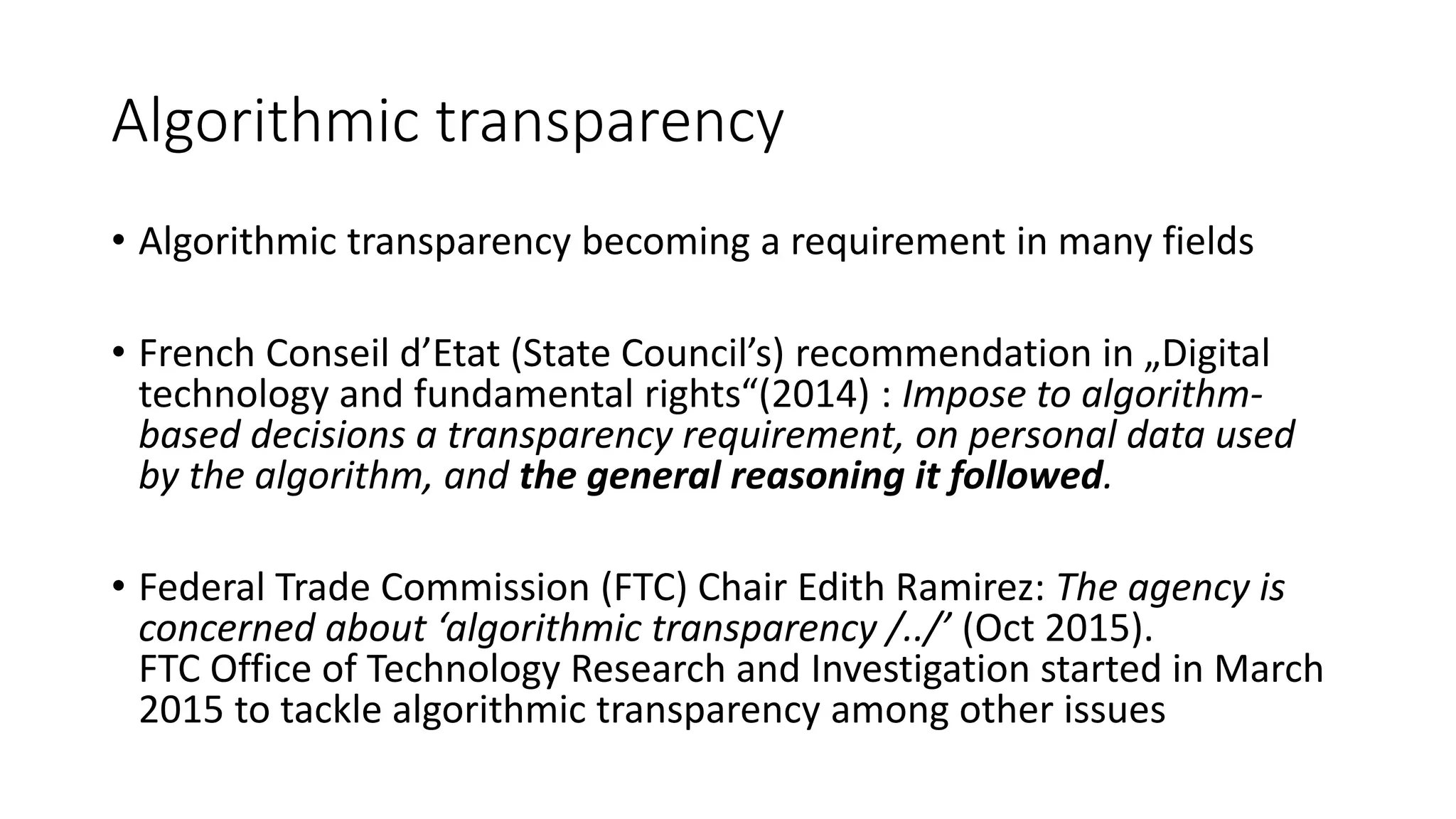
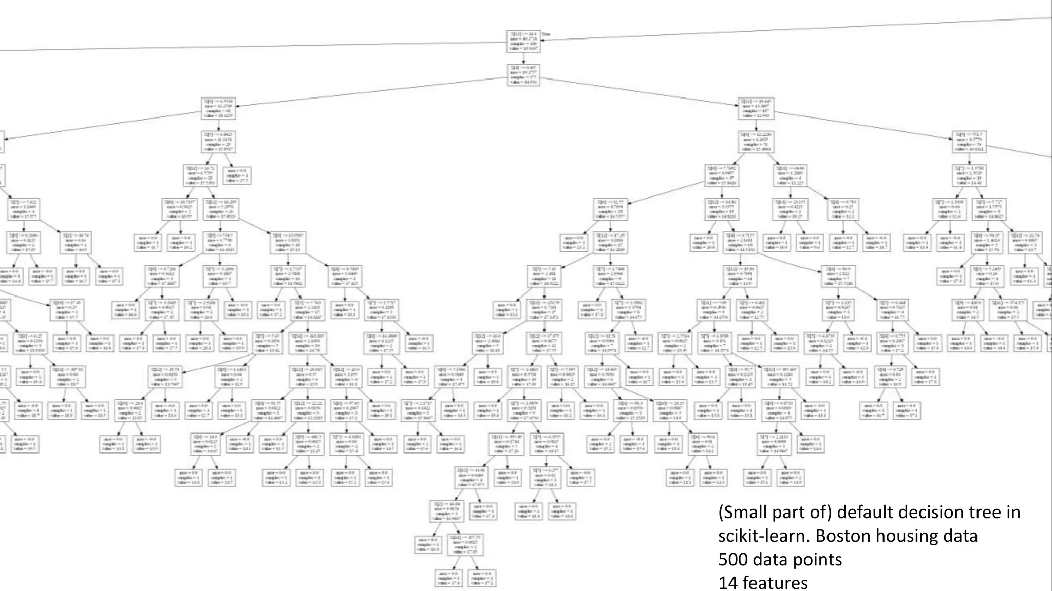
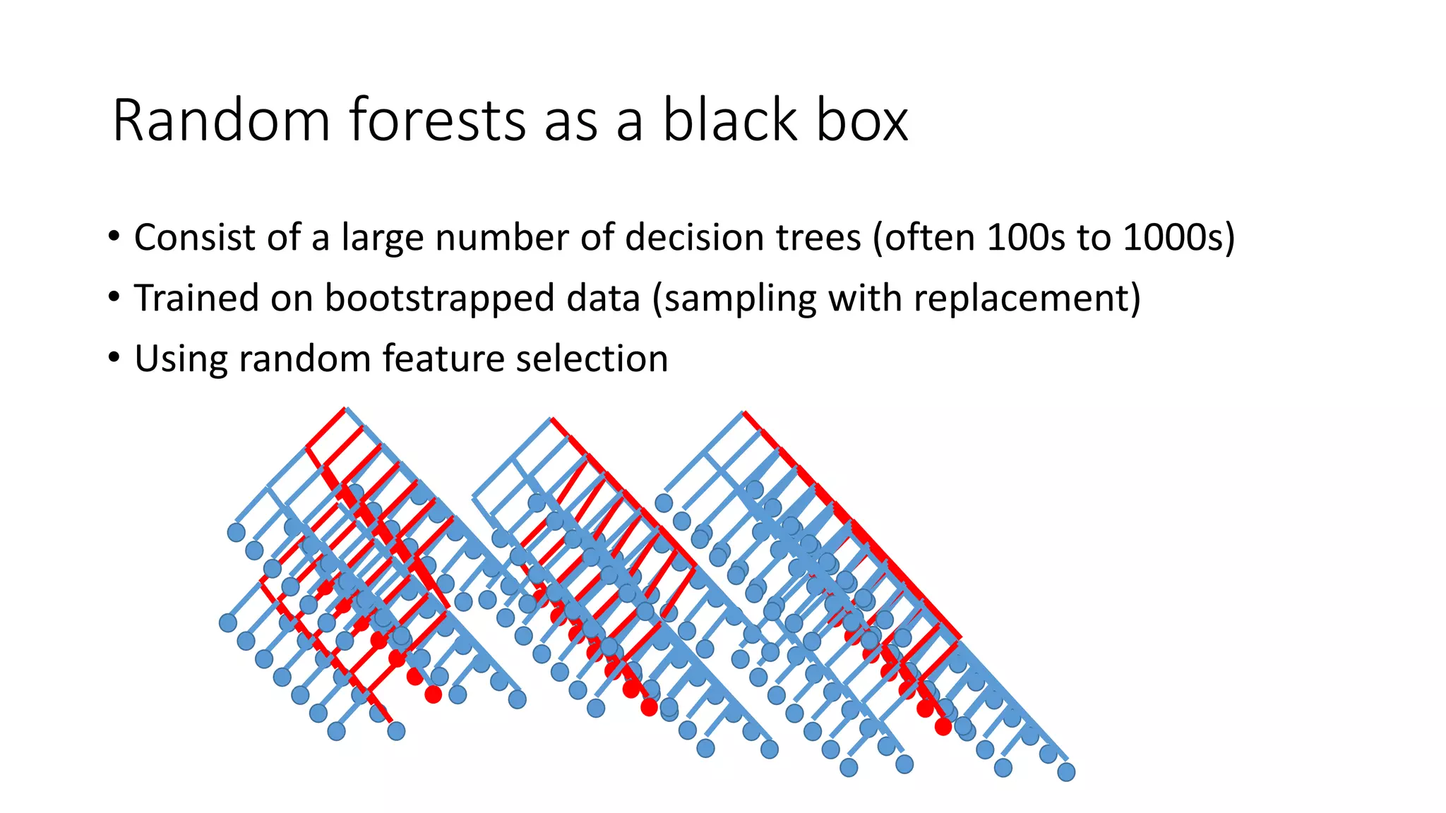
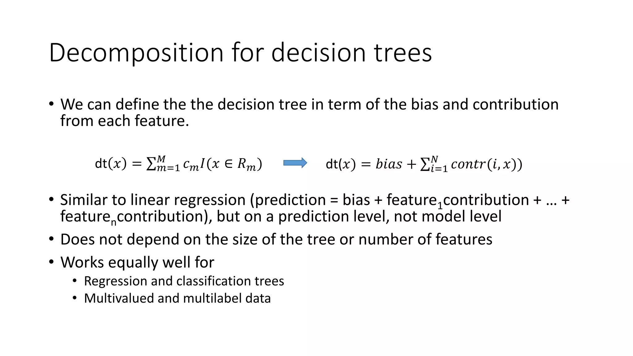
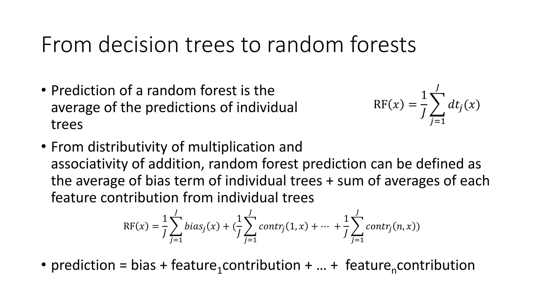
This document discusses interpreting machine learning models and summarizes techniques for interpreting random forests. Random forests are considered "black boxes" due to their complexity but their predictions can be explained by decomposing them into mathematically exact feature contributions. Decision trees can also be interpreted by defining the prediction as a bias plus the contributions from each feature along the decision path. This operational view of decision trees can be extended to interpret random forest predictions despite their complexity.

1. Interpreting machine
learning models
or how to turn a random forest into a white box
Ando Saabas

2. About me
• Senior applied scientist at Microsoft,
• Using ML and statistics to improve call quality in Skype
• Various projects on user engagement modelling, Skype user graph analysis,
call reliability modelling, traffic shaping detection
• Blogging on data science and ML @ http://blog.datadive.net/

3. Machine learning and model interpretation
• Machine learning studies algorithms that learn from data and make
predictions
• Learning algorithms are about correlations in the data
• In contrast, in data science and data mining, understanding causality
is essential
• Applying domain knowledge requires understanding and interpreting
models

4. Usefulness of model interpretation
• Often, we need to understand individual predictions a model is
making.
For example a model may
• Recommend a treatment for a patient or estimate a disease to be
likely. The doctor needs to understand the reasoning.
• Classify a user as a scammer, but the user disputes it. The fraud
analyst needs to understand why the model made the classification.
• Predict that a video call will be graded poorly by the user. The
engineer needs to understand why this type of call was considered
problematic.

5. Usefulness of model interpretation cont.
• Understanding differences on a dataset level.
• Why is a new software release receiving poorer feedback from customers
when compared to the previous one?
• Why are grain yields in one region higher than the other?
• Debugging models. A model that worked earlier is giving unexpected
results on newer data.

6. Algorithmic transparency
• Algorithmic transparency becoming a requirement in many fields
• French Conseil d’Etat (State Council’s) recommendation in „Digital
technology and fundamental rights“(2014) : Impose to algorithm-
based decisions a transparency requirement, on personal data used
by the algorithm, and the general reasoning it followed.
• Federal Trade Commission (FTC) Chair Edith Ramirez: The agency is
concerned about ‘algorithmic transparency /../’ (Oct 2015).
FTC Office of Technology Research and Investigation started in March
2015 to tackle algorithmic transparency among other issues

7. Interpretable models
• Traditionally, two types of (mainstream) models considered when
interpretability is required
• Linear models (linear and logistic regression)
• 𝑌 = 𝑎 + 𝑏1 𝑥1 + ⋯ + 𝑏 𝑛 𝑥 𝑛
• heart_disease = 0.08*tobacco + 0.043*age + 0.939*famhist + ...
(from Elements of statistical learning)
• Decision trees Family hist
Tobacco
Age > 60
Yes No
60% 20%40% 30%

8. Example: heart disease risk prediction
• Essentially a linear model
with integer coefficients
• Easy for a doctor to follow
and explain
From National Heart, Lung and Blood
Institute.

9. Linear models have drawbacks
• Underlying data is often non-linear
• Feature binning: potentially massive
increase in number of features
• Basis expansion (non-linear transfor-
mations of underlying features)
In both cases performance will be traded for interpretability
𝑌 = 2𝑥1 + 𝑥2 − 3𝑥3
𝑌 = 2𝑥1
2 + 3𝑥1 − log 𝑥2 + 𝑥2 𝑥3 + …
vs

10. Decision trees
• Decision trees can fit to non-linear data
• Work well with both categorical and continuous data, classification
and regression
• Easy to understand
Rooms < 3
Built_year < 2008
Crime rate < 3
35,00045,000
Floor < 2
55,00030,000
70,000
52,000
Crime_rate < 5
Yes No

11. (Small part of) default decision tree in
scikit-learn. Boston housing data
500 data points
14 features

12. Decision trees
• Decision trees are understandable only when they are (very) small
• Tree of depth n has up 2n leaves and 2n -1 internal nodes. With depth 20, a
tree can have up to 1048576 leaves
• Previous slide had <200 nodes
• Additionally decision trees are high variance method – low
generalization, tend to overfit

13. Random forests
• Can learn non-linear relationships in the data well
• Robust to outliers
• Can deal with both continuous and categorical data
• Require very little input preparation (see previous three points)
• Fast to train and test, trivially parallelizable
• High accuracy even with minimal meta-optimization
• Considered to be a black box that is difficult or impossible to interpret

14. Random forests as a black box
• Consist of a large number of decision trees (often 100s to 1000s)
• Trained on bootstrapped data (sampling with replacement)
• Using random feature selection

15. Random forests as a black box
• "Black box models such as random forests can't quantify the impact of each
predictor to the predictions of the complex model“, in PRICAI 2014: Trends
in Artificial Intelligence
• Unfortunately, the random forest algorithm is a black box when it comes to
evaluating the impact of a single feature on the overall performance. In
Advances in Natural Language Processing 2014
• “(Random forest model) is close to a black box in the sense that it uses 810
features /../ reduction in the number of features would allow an operator
to study individual decisions to have a rough idea how the global decision
could have been made”. In Advances in Data Mining: Applications and
Theoretical Aspects: 2014

16. Understanding the model vs the predictions
• Keep in mind, we want to understand why a particular decision was
made. Not necessarily every detail of the full model
• As an analogy, we don’t need to understand how a brain works to
understand why a person made a particular a decision: simple
explanation can be sufficient
• Ultimately, as ML models get more complex and powerful, hoping to
understand the models themselves is doomed to failure
• We should strive to make models explain their decisions

17. Turning the black box into a white box
• In fact, random forest predictions can be explained and interpreted,
by decomposing predictions into mathematically exact feature
contributions
• Independently of the
• number of features
• number of trees
• depth of the trees

18. • Classical definition (from Elements of statistical learning)
• Tree divides the feature space into M regions Rm (one for each leaf)
• Prediction for feature vector x is the constant cm associated with region Rm the
vector x belongs to
𝑑𝑡 𝑥 =
𝑚=1
𝑀
𝑐 𝑚 𝐼(𝑥 ∈ 𝑅 𝑚)
Revisiting decision trees

19. Example decision tree – predicting apartment
prices
Rooms < 3
Crime rate < 3
35,00045,000
Floor < 2
55,00030,000
70,000
52,000
Crime_rate < 5
Yes No
Built_year > 2008

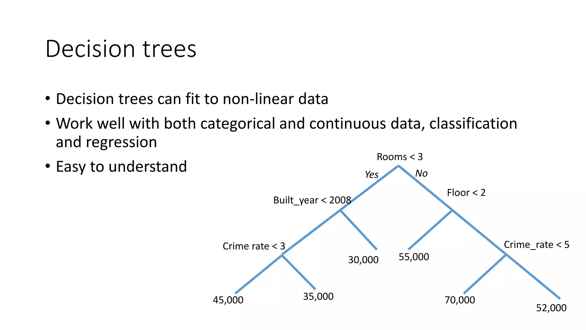
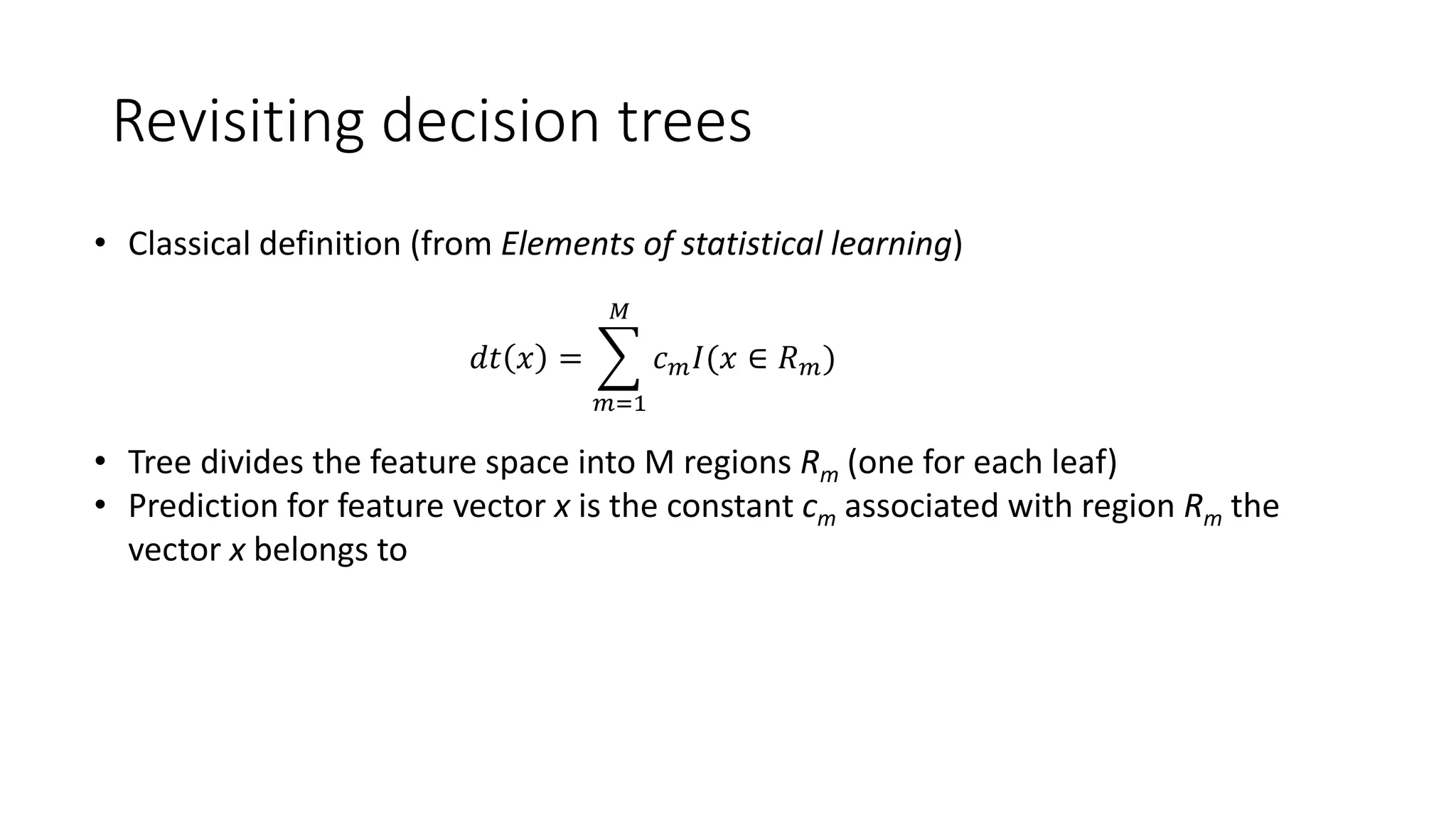
20. Estimating apartment prices
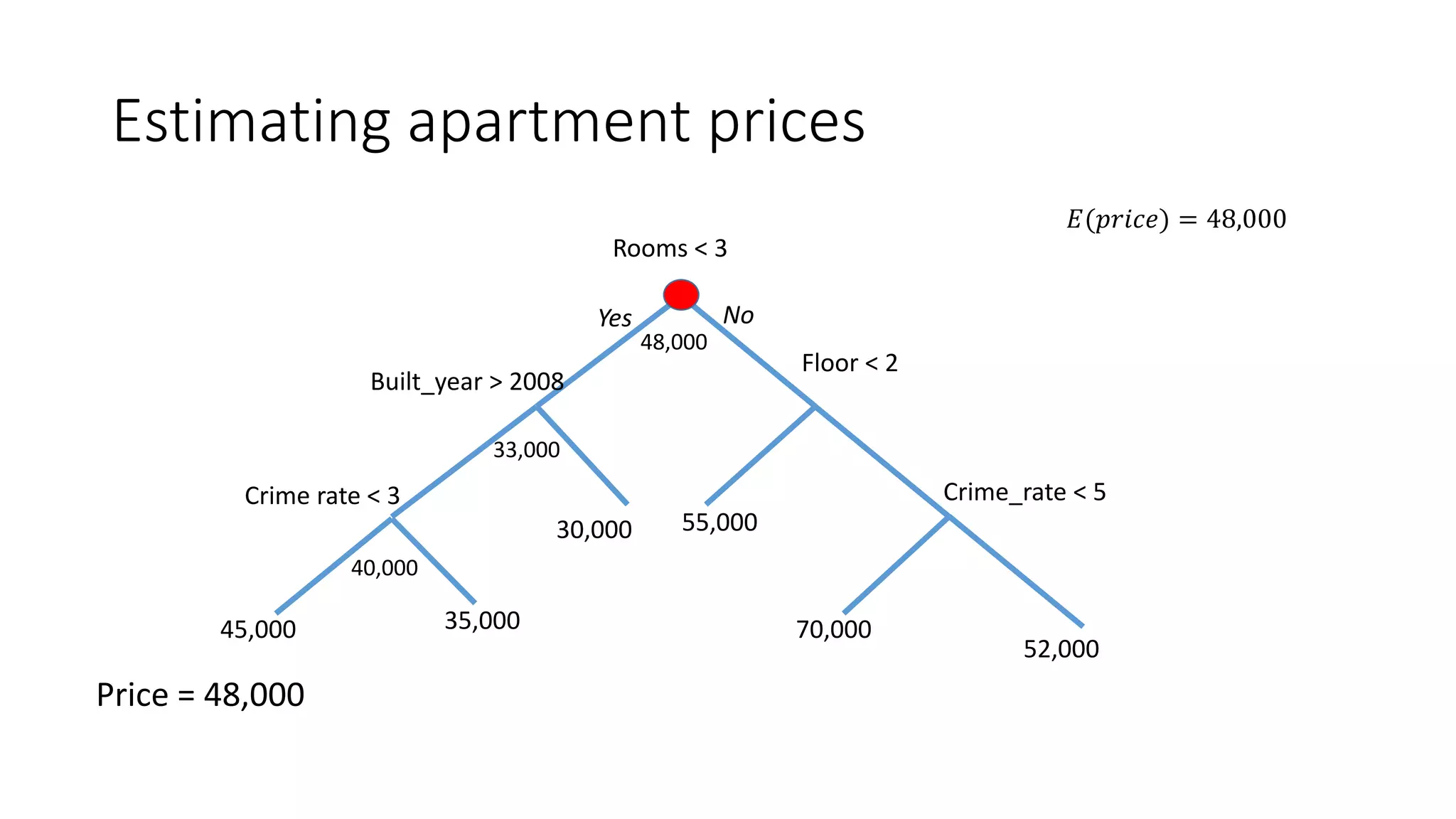
Assume an apartment [2 rooms; Built in 2010; Neighborhood crime rate: 5]
We walk the tree to obtain the price
Rooms < 3
Floor < 2
55,00030,000
70,000
52,000
Crime_rate < 5
Yes No
Crime rate < 3
35,00045,000
Built_year > 2008

21. Estimating apartment prices
[2 rooms; Built in 2010; Neighborhood crime rate: 5]
Rooms < 3
Floor < 2
55,00030,000
70,000
52,000
Crime_rate < 5
Yes No
Built_year > 2008
Crime rate < 3
35,00045,000

22. Estimating apartment prices
[2 rooms; Built in 2010; Neighborhood crime rate: 5]
Rooms < 3
Floor < 2
55,00030,000
70,000
52,000
Crime_rate < 5
Yes No
Built_year > 2008
Crime rate < 3
35,00045,000

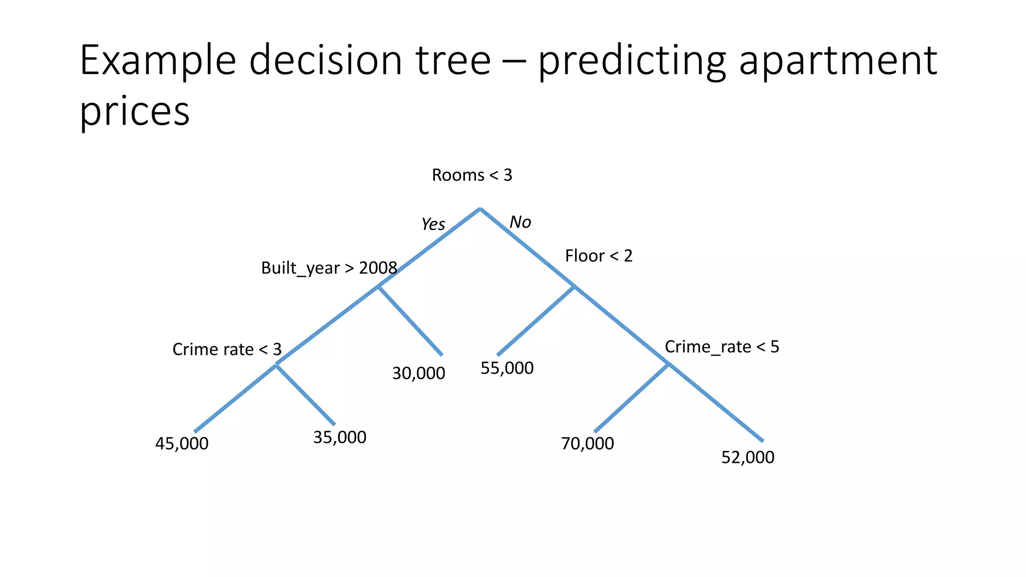
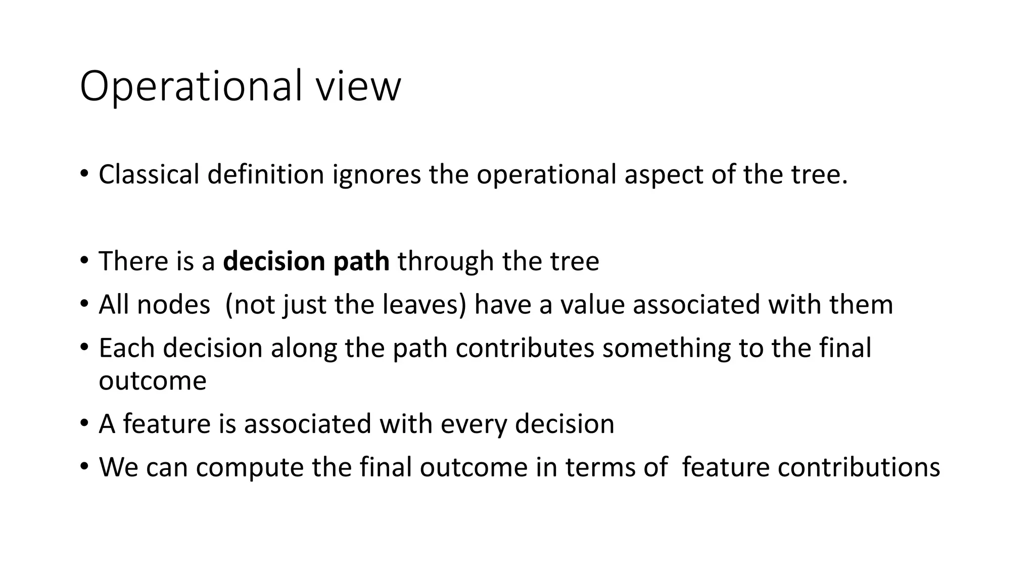
23. Estimating apartment prices
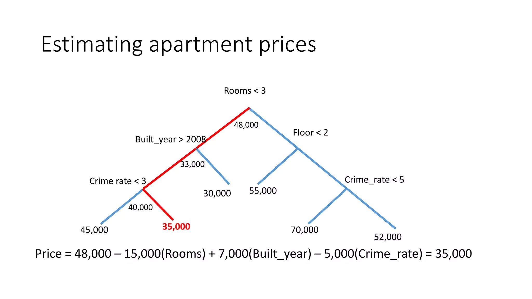
Prediction: 35,000 Path taken: Rooms < 3, Built_year > 2008, Crime_rate < 3
[2 rooms; Built in 2010; Neighborhood crime rate: 5]
Rooms < 3
Floor < 2
55,00030,000
70,000
52,000
Crime_rate < 5Crime rate < 3
35,00045,000
Yes No
Built_year > 2008

24. Operational view
• Classical definition ignores the operational aspect of the tree.
• There is a decision path through the tree
• All nodes (not just the leaves) have a value associated with them
• Each decision along the path contributes something to the final
outcome
• A feature is associated with every decision
• We can compute the final outcome in terms of feature contributions

25. Estimating apartment prices
Rooms < 3
Floor < 2
55,00030,000
70,000
52,000
Crime_rate < 5
Yes No
Built_year > 2008
Crime rate < 3
35,00045,000
48,000
33,000
40,000

26. Estimating apartment prices
Price = 48,000
Rooms < 3
Floor < 2
55,00030,000
70,000
52,000
Crime_rate < 5
Yes No
Built_year > 2008
Crime rate < 3
35,00045,000
48,000
33,000
40,000
𝐸(𝑝𝑟𝑖𝑐𝑒) = 48,000

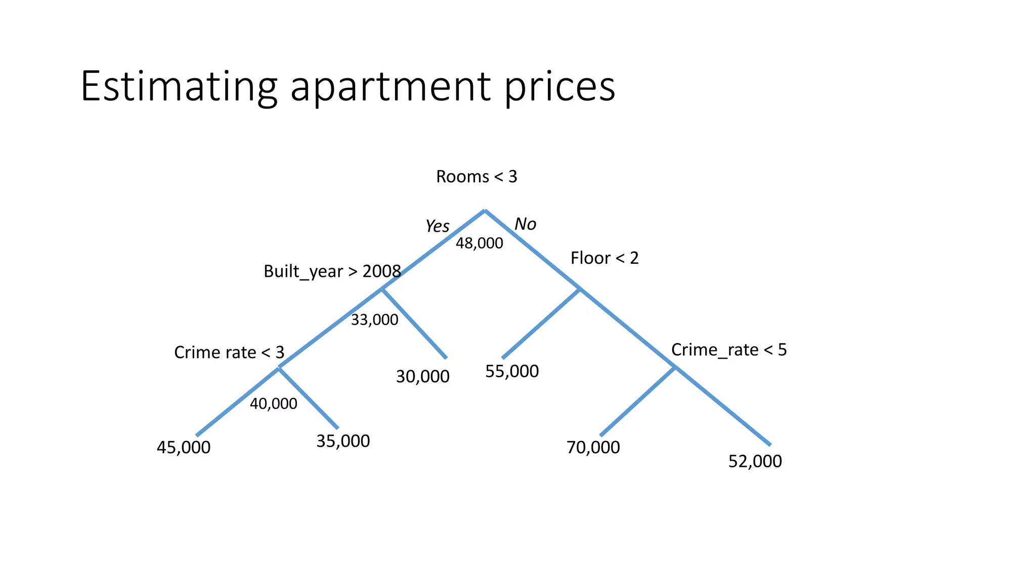
27. Estimating apartment prices
[2 rooms]
Rooms < 3
Floor < 2
55,00030,000
70,000
52,000
Crime_rate < 5
Yes No
Built_year > 2008
Crime rate < 3
35,00045,000
48,000
33,000
40,000
Price = 48,000 – 15,000(Rooms)
𝐸(𝑝𝑟𝑖𝑐𝑒|𝑟𝑜𝑜𝑚𝑠 < 3) = 33,000

28. Estimating apartment prices
Rooms < 3
Floor < 2
55,00030,000
70,000
52,000
Crime_rate < 5
Yes No
Built_year > 2008
Crime rate < 3
35,00045,000
48,000
33,000
40,000
Price = 48,000 – 15,000(Rooms) + 7,000(Built_year)
[Built 2010]

29. Estimating apartment prices
Rooms < 3
Floor < 2
55,00030,000
70,000
52,000
Crime_rate < 5
Built_year > 2008
Crime rate < 3
35,00045,000
48,000
33,000
40,000
Price = 48,000 – 15,000(Rooms) + 7,000(Built_year) – 5,000(Crime_rate)
[Crime rate 5]

30. Estimating apartment prices
Rooms < 3
Floor < 2
55,00030,000
70,000
52,000
Crime_rate < 5
Built_year > 2008
Crime rate < 3
35,00045,000
48,000
33,000
40,000
Price = 48,000 – 15,000(Rooms) + 7,000(Built_year) – 5,000(Crime_rate) = 35,000

31. • We can define the the decision tree in term of the bias and contribution
from each feature.
• Similar to linear regression (prediction = bias + feature1contribution + … +
featurencontribution), but on a prediction level, not model level
• Does not depend on the size of the tree or number of features
• Works equally well for
• Regression and classification trees
• Multivalued and multilabel data
Decomposition for decision trees
dt(𝑥) = 𝑏𝑖𝑎𝑠 + 𝑖=1
𝑁
𝑐𝑜𝑛𝑡𝑟(𝑖, 𝑥))dt 𝑥 = 𝑚=1
𝑀
𝑐 𝑚 𝐼(𝑥 ∈ 𝑅 𝑚)

32. Deeper inspections
• We can have more fine grained definition in addition to pure feature
contributions
• Separate negative and positive contributions
• Contribution from decisions (floor = 1  -15000)
• Contribution from interactions (floor == 1 & has_terrace  3000)
• etc
• Number of features typically not a concern because of the long tail.
In practice, top 10 features contribute the vast majority of the overall
deviation from the mean

33. From decision trees to random forests
• Prediction of a random forest is the
average of the predictions of individual
trees
• From distributivity of multiplication and
associativity of addition, random forest prediction can be defined as
the average of bias term of individual trees + sum of averages of each
feature contribution from individual trees
• prediction = bias + feature1contribution + … + featurencontribution
RF 𝑥 =
1
𝐽
𝑗=1
𝐽
𝑑𝑡𝑗(𝑥)
RF 𝑥 =
1
𝐽
𝑗=1
𝐽
𝑏𝑖𝑎𝑠𝑗 𝑥 + (
1
𝐽
𝑗=1
𝐽
𝑐𝑜𝑛𝑡𝑟𝑗 1, 𝑥 + ⋯ +
1
𝐽
𝑗=1
𝐽
𝑐𝑜𝑛𝑡𝑟𝑗 𝑛, 𝑥 )

34. Random forest interpretation in Scikit-Learn
• Path walking in general no supported by ML libraries
• Scikit-Learn: one of the most popular Python (and overall) ML
libraries
• Patch since 0.17 (released Nov 8 2015) to include values/predictions
at each node: allows walking the tree paths and collecting values
along the way
• Treeintepreter library for decomposing the predictions
• https://github.com/andosa/treeinterpreter
• pip install treeinterpreter
• Supports both decision tree and random forest classes, regression
and classification

35. Using treeinterpreter
• Decomposing predictions is a one-liner
from treeinterpreter import treeinterpreter as ti
rf = RandomForestRegressor()
rf.fit(trainX,trainY)
prediction, bias, contributions = ti.predict(rf, testX)
#prediction == bias + contributions
assert(numpy.allclose(prediction, bias + np.sum(contributions, axis=1)))

36. Decomposing a prediction – boston housing
data
prediction, bias, contributions = ti.predict(rf, boston.data)
>> prediction[0]
30.69
>> bias[0]
25.588
>> sorted(zip(contributions[0], boston.feature_names),
>> key=lambda x: -abs(x[0]))
[(4.3387165697195558, 'RM'),
(-1.0771391053864874, 'TAX'),
(1.0207116129073213, 'LSTAT'),
(0.38890774812797702, 'AGE'),
(0.38381481481481539, 'ZN'),
(-0.10397222222222205, 'CRIM'),
(-0.091520697167756987, 'NOX')
...

37. Conclusions
• Model interpretation can be very beneficial for ML and data science
practitioners in many tasks
• No need to understand the full model in many/most cases: explanation of
decisions sufficient
• Random forests can be turned from black box into a white box
• Each prediction can decomposed into bias and feature contribution terms
• Python library available for scikit-learn at
https://github.com/andosa/treeinterpreter
or pip install treeinterpreter
• Subscribe to http://blog.datadive.net/
• Follow @crossentropy