Pydata presentation

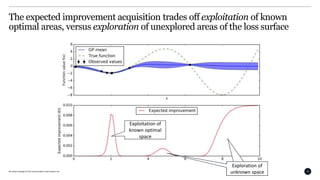
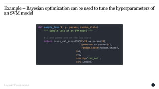
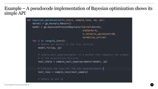
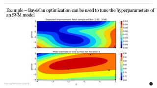
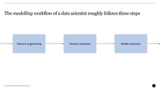
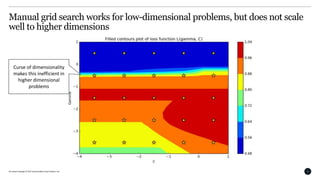
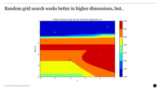
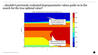
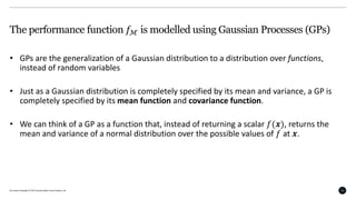
All content Copyright © 2017 QuantumBlack Visual Analytics Ltd.
Bayesian optimization
PyData London 2017
6th of May, 2017
Thomas Huijskens

All content Copyright © 2017 QuantumBlack Visual Analytics Ltd. 2
The modelling workflow of a data scientist roughly follows three steps
Feature engineering Feature selection Model selection

In this talk, we will focus on the last step of this workflow
Feature engineering Model selection
Focus of this talk
Feature selection

Most models have a number of hyperparameters that need to be chosen a
priori..
• Typically, we want to optimize some performance metric 𝑓ℳ for a model ℳ, on a hold-out
set of data.
• The model ℳ has some hyperparameters 𝜃 that we need to specify, and the performance
of ℳ is highly dependent on the settings of 𝜃.
• Example: For a classification problem, ℳ could be a support vector machine, and the
performance metric 𝑓ℳ could be the out-of-sample AUC.
• Because the performance of the SVM depends on hyperparameters 𝜃, the metric 𝑓ℳ
depends on 𝜃 as well.

𝑓ℳ 𝜃 𝐷)
Learner ℳ
Performance
function 𝑓
𝑓 depends on the hyperparameters 𝜃 of
the model ℳ
.. and our goal is to find the values of 𝜃 for which the value of the (out-of-
sample) performance 𝑓ℳ is optimal
𝑓 is conditional on the
data 𝐷

Manual grid search works for low-dimensional problems, but does not scale
well to higher dimensions
Curse of dimensionality
makes this inefficient in
higher dimensional
problems

Random grid search works better in higher dimensions, but..

.. shouldn't previously evaluated hyperparameter values guide us in the
search for the true optimal value?
Low values of L here,
should probably not
focus in this area
High values of L here,
should probably focus
in this area

Bayesian optimization

Bayesian optimization is only beneficial in certain situations
In Bayesian optimization, we are building a probabilistic model for the performance metric
𝑓ℳ(𝜃). This introduces computational overhead.
As a result, applying Bayesian optimization only really makes sense if
• The number of hyperparameters is very high (𝜃 is of high dimension); or
• It is computationally very expensive to evaluate 𝑓ℳ(𝜃) for a single point 𝜃.

Evaluate performance
of learner f with
parameters 𝜃
Update current belief
of loss surface of the
learner f
Choose 𝜃 that
maximises some
utility over the
current belief
The classic Bayesian optimization algorithm consists of three steps
𝑓 | 𝑦 𝑛𝑒𝑤
𝑦 𝑛𝑒𝑤 = 𝑓 𝜃 𝑛𝑒𝑤
𝜃 𝑛𝑒𝑤

of learner f with
parameters 𝜃
learner f
Choose 𝜃 that
maximises some
utility over the
current belief
𝜃 𝑛𝑒𝑤

The performance function 𝑓ℳ is modelled using Gaussian Processes (GPs)
• GPs are the generalization of a Gaussian distribution to a distribution over functions,
instead of random variables
• Just as a Gaussian distribution is completely specified by its mean and variance, a GP is
completely specified by its mean function and covariance function.
• We can think of a GP as a function that, instead of returning a scalar 𝑓(𝒙), returns the
mean and variance of a normal distribution over the possible values of 𝑓 at 𝒙.

GPs are the generalization of a Gaussian distribution to a distribution over
functions, instead of random variables1
1A Tutorial on Bayesian Optimization of Expensive Cost Functions, with Application to Active User Modeling and Hierarchical Reinforcement Learning, Eric Brochu, Vlad M. Cora, Nando de Freitas, 2010. https://arxiv.org/abs/1012.2599

of learner f with
parameters 𝜃
learner f
Choose 𝜃 that
maximises some
utility over the
current belief
𝜃 𝑛𝑒𝑤

How do we use our current belief to make a good guess about what point to
evaluate next?

Acquisition functions are used to formalize what constitutes a ”best guess”
𝐸𝐼 𝜃 = 𝔼[max
𝜃
0, 𝑓ℳ 𝜃 − 𝑓ℳ 𝜃 ] ,
𝜃 𝑛𝑒𝑤 = argmax
𝜃
𝐸𝐼(𝜃)

The expected improvement acquisition function can be evaluated analytically
𝐸𝐼 𝜃 =
𝜇 𝜃 − 𝑓 𝜃 𝛷 𝑍 + 𝜎(𝜃)𝜙(𝑍), 𝜎 𝜃 > 0
0, 𝜎 𝜃 = 0
,
𝑍 =
𝜇 𝜃 − 𝑓( 𝜃)
𝜎(𝜃)

The expected improvement acquisition trades off exploitation of known
optimal areas, versus exploration of unexplored areas of the loss surface
Exploitation of
known optimal
space
Exploration of
unknown space
Exploration of
unknown space

of learner f with
parameters 𝜃
learner f
Choose 𝜃 that
maximises some
utility over the
current belief
𝜃 𝑛𝑒𝑤

How do we use this in real-life?

Example – Bayesian optimization can be used to tune the hyperparameters of
an SVM model

Example – A pseudocode implementation of Bayesian optimization shows its
simple API

an SVM model

GPs can not be used as a simple black-box, and some care must be taken
1. Choose an appropriate scale for your hyperparameters: For parameters like a learning
rate, or regularization term, it makes more sense to sample on the log-uniform domain,
instead of the uniform domain.
2. Choose the kernel of the GP carefully: Each kernel implicitly assumes different properties
on the loss function, in terms of differentiability and periodicity.

Multiple production-ready, and open-source, modules for Bayesian
optimization are available online
1. Spearmint
2. Hyperopt
3. MOE
4. Hyperband (model-free)
5. SMAC (model-free)

Pydata presentation

More Related Content

What's hot

Similar to Pydata presentation

Recently uploaded

Pydata presentation

Editor's Notes