Download as PDF, PPTX


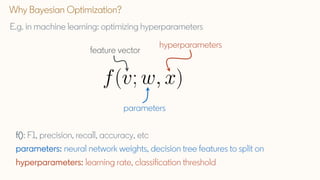


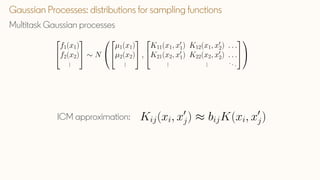


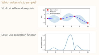


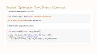


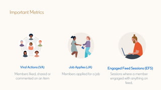


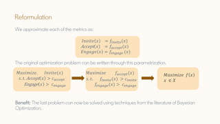
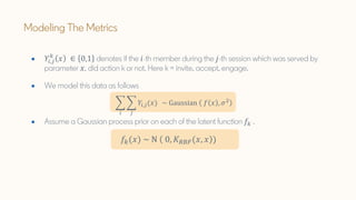
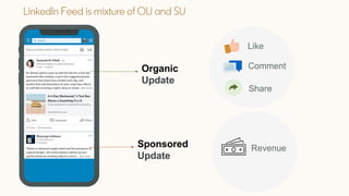


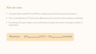


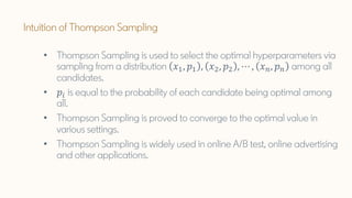


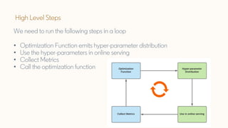


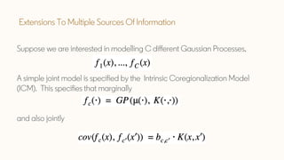


The document discusses Bayesian optimization techniques for balancing metrics in recommender systems, with a focus on real-world applications like LinkedIn's feed system. It covers the introduction of Bayesian optimization, practical considerations, and the integration of Gaussian processes for optimizing hyperparameters and neural architecture search. Additionally, it highlights the importance of balancing various engagement metrics to improve user interaction and revenue generation.