A Machine Learning Framework for Materials
Knowledge Systems
Surya R. Kalidindi
Funding: DoD, NIST
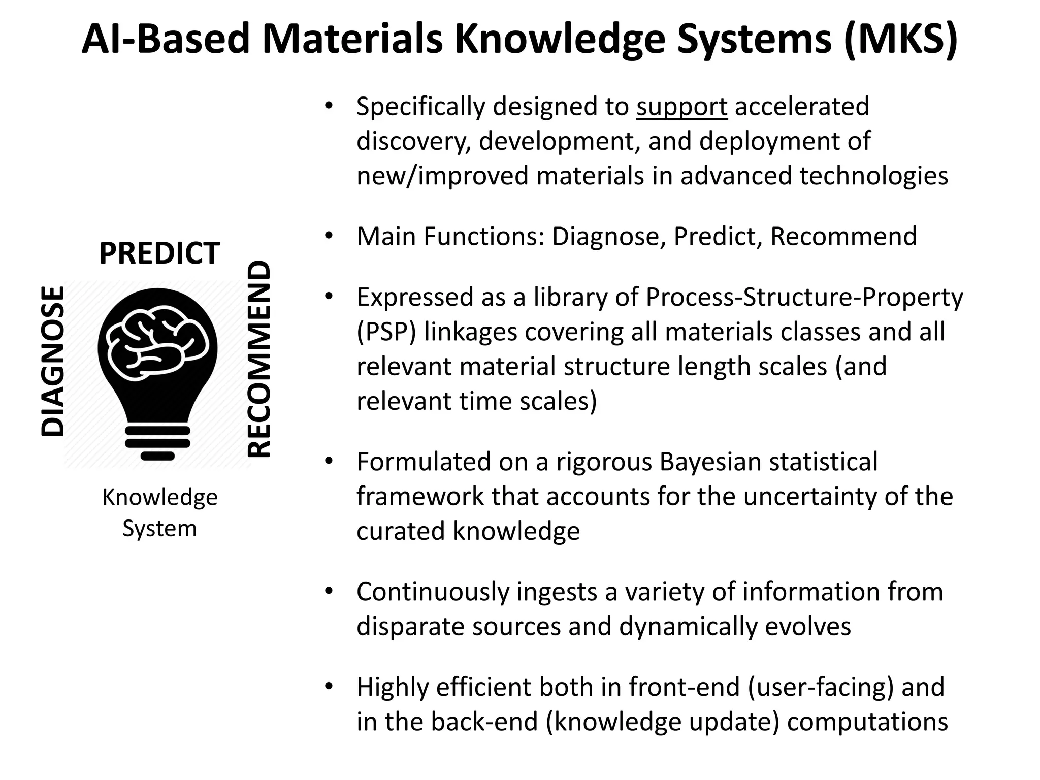
AI-Based Materials Knowledge Systems (MKS)
Knowledge
System
PREDICT
DIAGNOSE
RECOMMEND
• Specifically designed to support accelerated
discovery, development, and deployment of
new/improved materials in advanced technologies
• Main Functions: Diagnose, Predict, Recommend
• Expressed as a library of Process-Structure-Property
(PSP) linkages covering all materials classes and all
relevant material structure length scales (and
relevant time scales)
• Formulated on a rigorous Bayesian statistical
framework that accounts for the uncertainty of the
curated knowledge
• Continuously ingests a variety of information from
disparate sources and dynamically evolves
• Highly efficient both in front-end (user-facing) and
in the back-end (knowledge update) computations
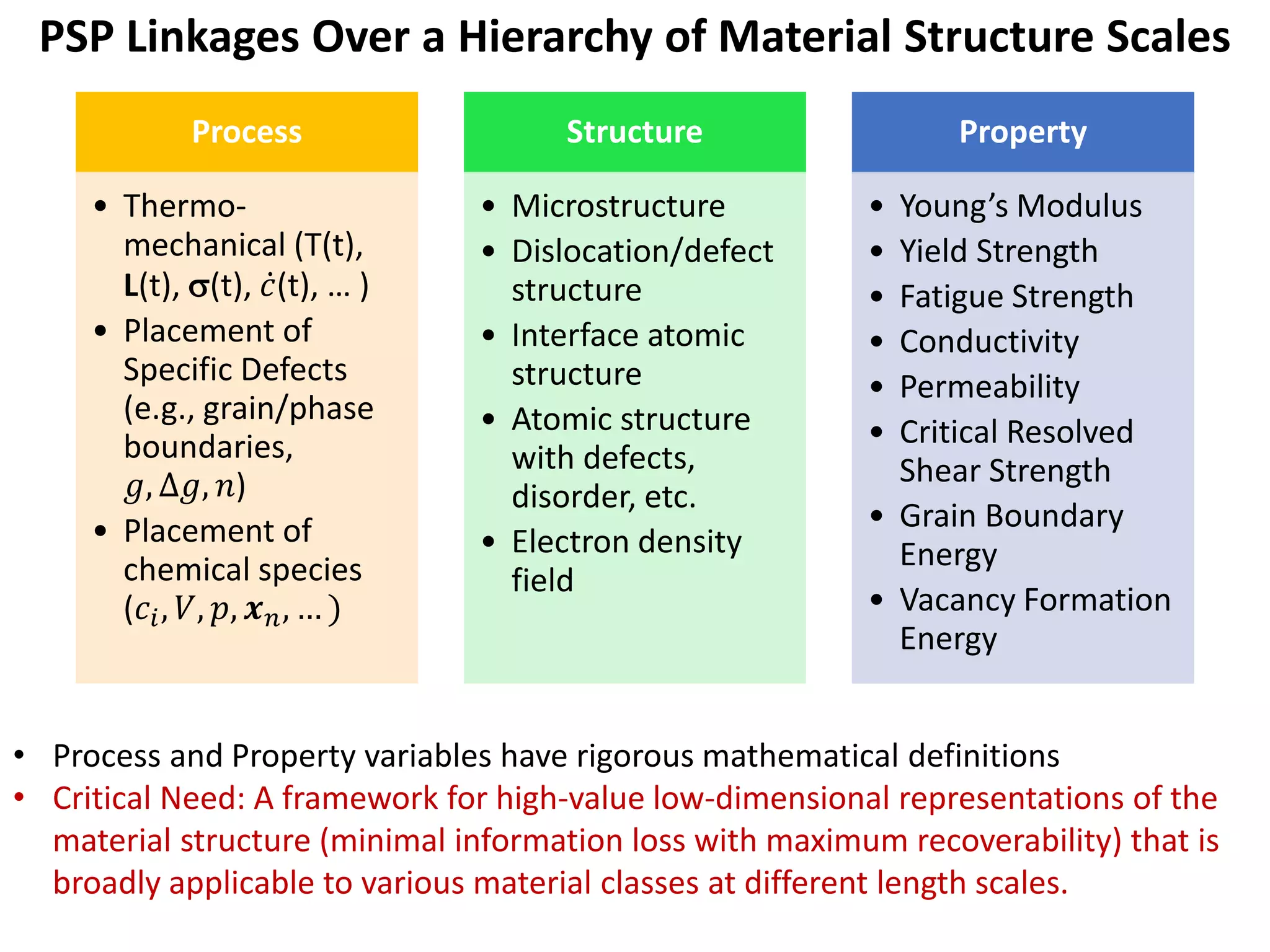
Process
• Thermo-
mechanical (T(t),
L(t), σ(t), ̇𝑐𝑐(t), … )
• Placement of
Specific Defects
(e.g., grain/phase
boundaries,
𝑔𝑔, ∆𝑔𝑔, 𝑛𝑛)
• Placement of
chemical species
(𝑐𝑐𝑖𝑖, 𝑉𝑉, 𝑝𝑝, 𝒙𝒙𝑛𝑛, … )
Structure
• Microstructure
• Dislocation/defect
structure
• Interface atomic
structure
• Atomic structure
with defects,
disorder, etc.
• Electron density
field
Property
• Young’s Modulus
• Yield Strength
• Fatigue Strength
• Conductivity
• Permeability
• Critical Resolved
Shear Strength
• Grain Boundary
Energy
• Vacancy Formation
Energy
PSP Linkages Over a Hierarchy of Material Structure Scales
• Process and Property variables have rigorous mathematical definitions
• Critical Need: A framework for high-value low-dimensional representations of the
material structure (minimal information loss with maximum recoverability) that is
broadly applicable to various material classes at different length scales.
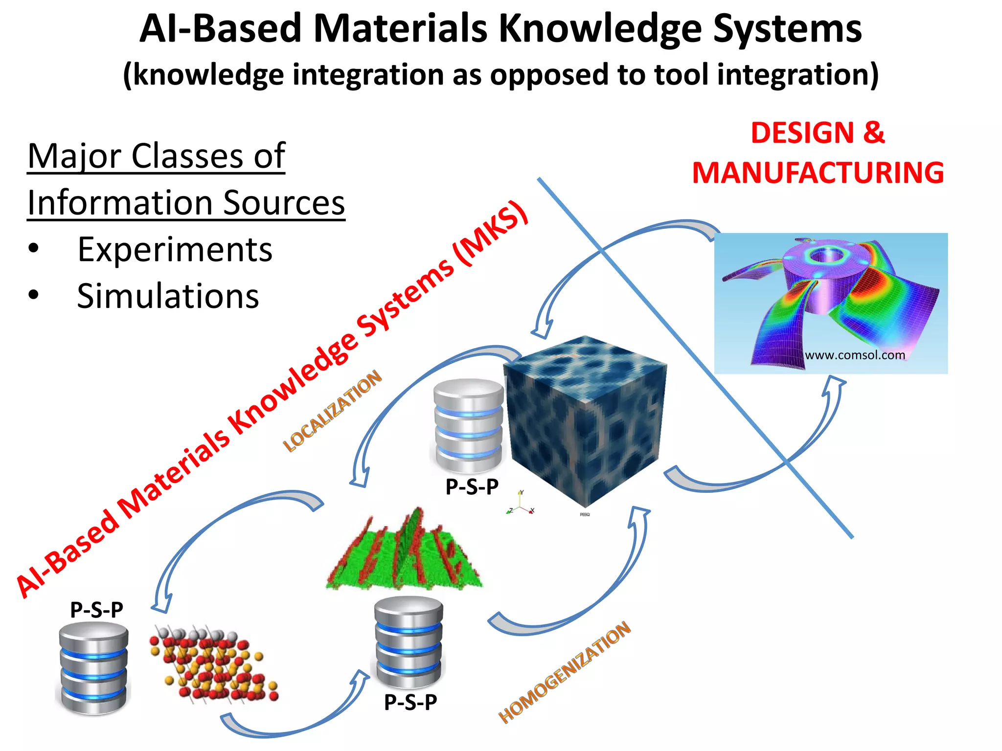
AI-Based Materials Knowledge Systems
(knowledge integration as opposed to tool integration)
www.comsol.com
DESIGN &
MANUFACTURING
P-S-P
P-S-P
P-S-P
Major Classes of
Information Sources
• Experiments
• Simulations
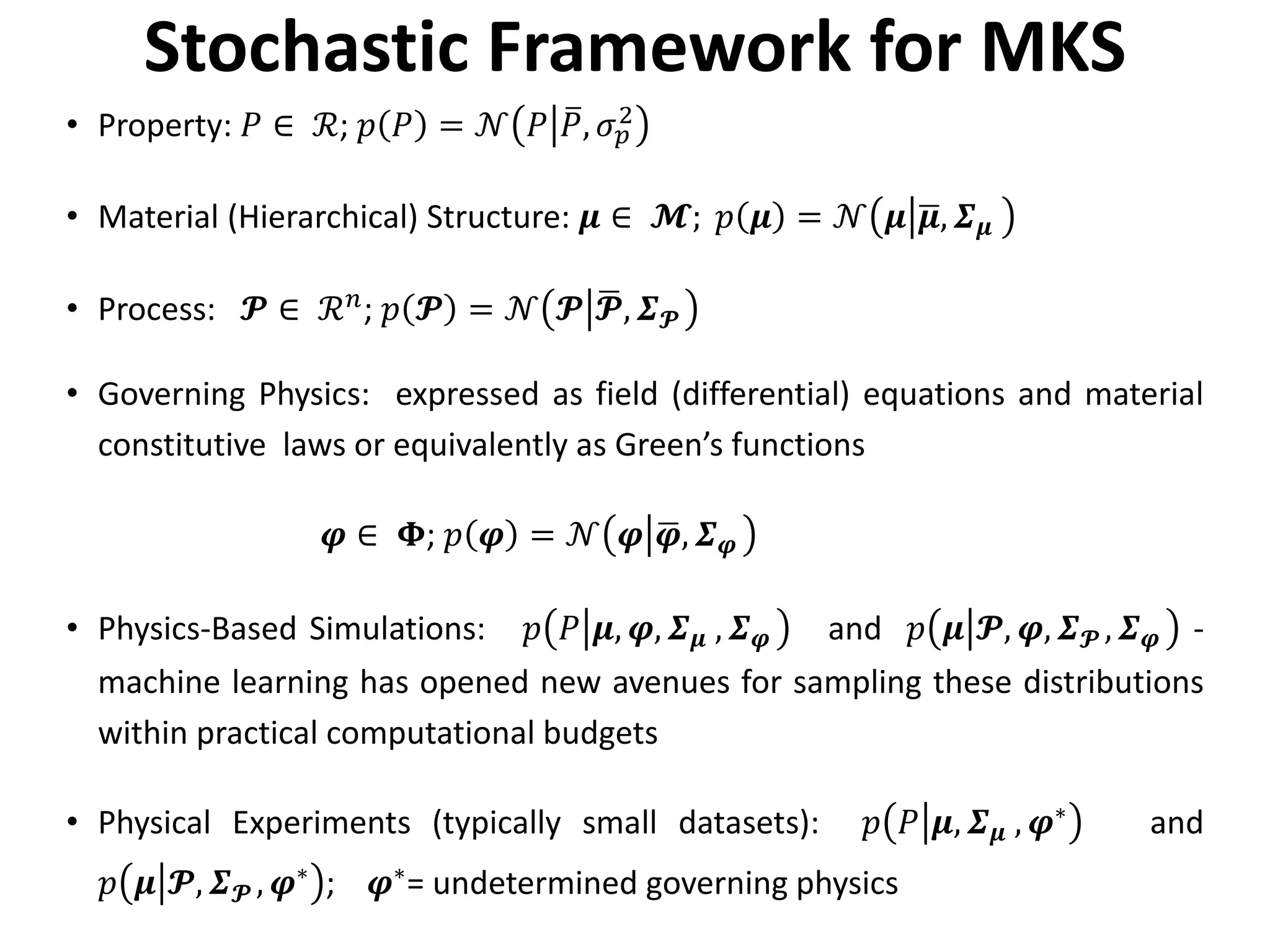
Stochastic Framework for MKS
• Property: 𝑃𝑃 ∈ ℛ; 𝑝𝑝 𝑃𝑃 = 𝒩𝒩 𝑃𝑃 �𝑃𝑃, 𝜎𝜎𝑝𝑝
2
• Material (Hierarchical) Structure: 𝝁𝝁 ∈ 𝓜𝓜; 𝑝𝑝 𝝁𝝁 = 𝒩𝒩 𝝁𝝁 �𝝁𝝁, 𝜮𝜮𝝁𝝁
• Process: 𝓟𝓟 ∈ ℛ𝑛𝑛
; 𝑝𝑝 𝓟𝓟 = 𝒩𝒩 𝓟𝓟 �𝓟𝓟, 𝜮𝜮𝓟𝓟
• Governing Physics: expressed as field (differential) equations and material
constitutive laws or equivalently as Green’s functions
𝝋𝝋 ∈ 𝚽𝚽; 𝑝𝑝 𝝋𝝋 = 𝒩𝒩 𝝋𝝋 �𝝋𝝋, 𝜮𝜮𝝋𝝋
• Physics-Based Simulations: 𝑝𝑝 𝑃𝑃 𝝁𝝁, 𝝋𝝋, 𝜮𝜮𝝁𝝁 , 𝜮𝜮𝝋𝝋 and 𝑝𝑝 𝝁𝝁 𝓟𝓟, 𝝋𝝋, 𝜮𝜮𝓟𝓟 , 𝜮𝜮𝝋𝝋 -
machine learning has opened new avenues for sampling these distributions
within practical computational budgets
• Physical Experiments (typically small datasets): 𝑝𝑝 𝑃𝑃 𝝁𝝁, 𝜮𝜮𝝁𝝁 , 𝝋𝝋∗ and
𝑝𝑝 𝝁𝝁 𝓟𝓟, 𝜮𝜮𝓟𝓟 , 𝝋𝝋∗
; 𝝋𝝋∗
= undetermined governing physics
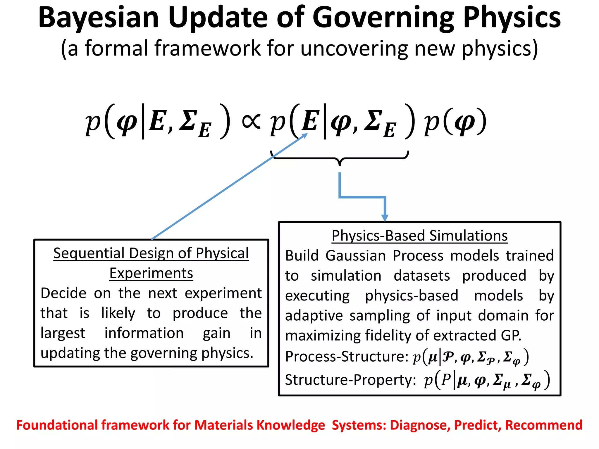
Bayesian Update of Governing Physics
(a formal framework for uncovering new physics)
𝑝𝑝 𝝋𝝋 𝑬𝑬, 𝜮𝜮𝑬𝑬 ∝ 𝑝𝑝 𝑬𝑬 𝝋𝝋, 𝜮𝜮𝑬𝑬 𝑝𝑝 𝝋𝝋
Physics-Based Simulations
Build Gaussian Process models trained
to simulation datasets produced by
executing physics-based models by
adaptive sampling of input domain for
maximizing fidelity of extracted GP.
Process-Structure: 𝑝𝑝 𝝁𝝁 𝓟𝓟, 𝝋𝝋, 𝜮𝜮𝓟𝓟 , 𝜮𝜮𝝋𝝋
Structure-Property: 𝑝𝑝 𝑃𝑃 𝝁𝝁, 𝝋𝝋, 𝜮𝜮𝝁𝝁 , 𝜮𝜮𝝋𝝋
Sequential Design of Physical
Experiments
Decide on the next experiment
that is likely to produce the
largest information gain in
updating the governing physics.
Foundational framework for Materials Knowledge Systems: Diagnose, Predict, Recommend
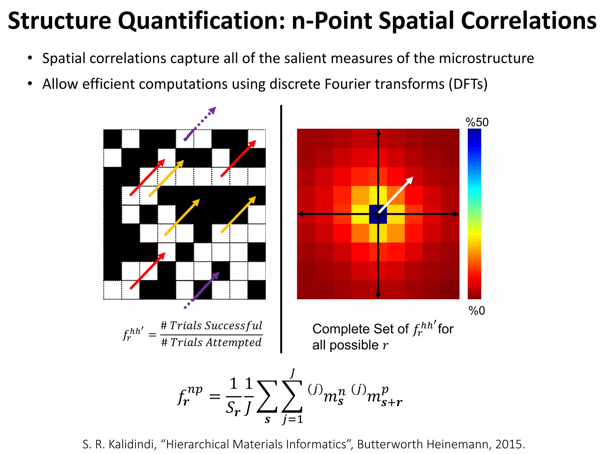
Structure Quantification: n-Point Spatial Correlations
• Spatial correlations capture all of the salient measures of the microstructure
• Allow efficient computations using discrete Fourier transforms (DFTs)
𝑓𝑓𝒓𝒓
𝑛𝑛𝑛𝑛
=
1
𝑆𝑆𝒓𝒓
1
𝐽𝐽
�
𝒔𝒔
�
𝑗𝑗=1
𝐽𝐽
(𝑗𝑗)
𝑚𝑚𝒔𝒔
𝑛𝑛 (𝑗𝑗)
𝑚𝑚𝒔𝒔+𝒓𝒓
𝑝𝑝
𝑓𝑓𝑟𝑟
ℎℎ′
=
# 𝑇𝑇𝑇𝑇𝑇𝑇𝑇𝑇𝑇𝑇𝑇𝑇 𝑆𝑆𝑆𝑆𝑆𝑆𝑆𝑆𝑆𝑆𝑆𝑆𝑆𝑆𝑆𝑆𝑆𝑆𝑆𝑆
# 𝑇𝑇𝑇𝑇𝑇𝑇𝑇𝑇𝑇𝑇𝑇𝑇 𝐴𝐴𝐴𝐴𝐴𝐴 𝐴𝐴𝐴𝐴𝐴𝐴𝐴𝐴𝐴𝐴𝐴𝐴
%50
%0
Complete Set of 𝑓𝑓𝑟𝑟
ℎℎ′
for
all possible 𝑟𝑟
S. R. Kalidindi, “Hierarchical Materials Informatics”, Butterworth Heinemann, 2015.
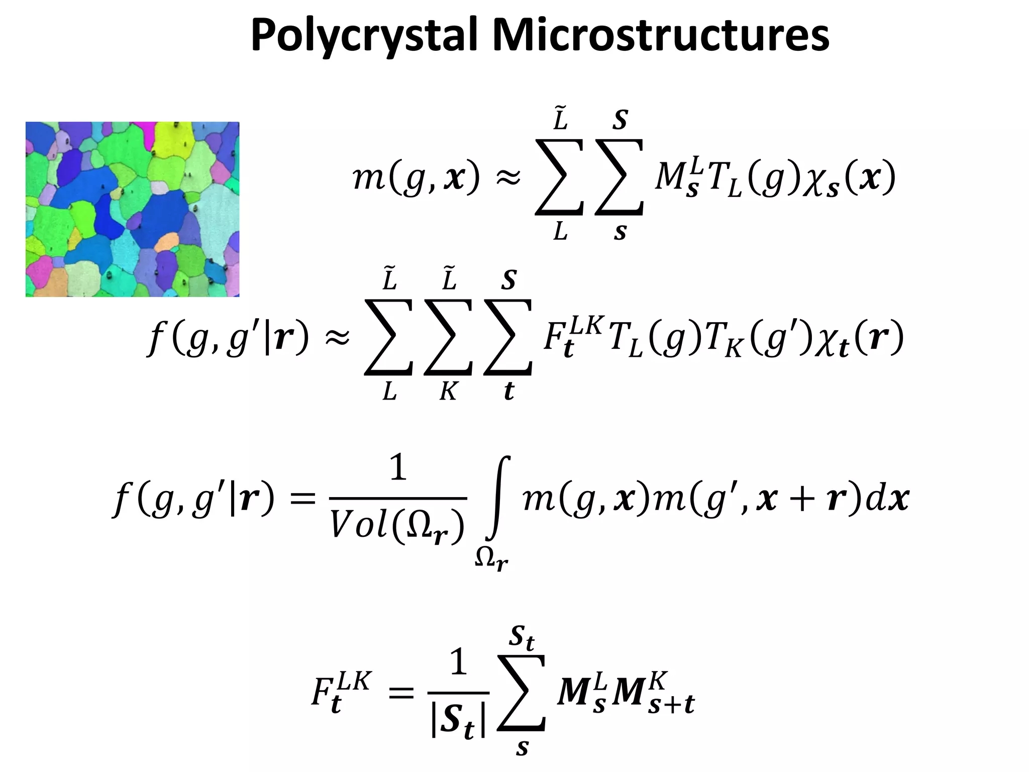
Polycrystal Microstructures
𝑚𝑚 𝑔𝑔, 𝒙𝒙 ≈ �
𝐿𝐿
�𝐿𝐿
�
𝒔𝒔
𝑺𝑺
𝑀𝑀𝒔𝒔
𝐿𝐿 𝑇𝑇𝐿𝐿 𝑔𝑔 𝜒𝜒𝒔𝒔 𝒙𝒙
𝑓𝑓 𝑔𝑔, 𝑔𝑔𝑔 𝒓𝒓 ≈ �
𝐿𝐿
�𝐿𝐿
�
𝐾𝐾
�𝐿𝐿
�
𝒕𝒕
𝑺𝑺
𝐹𝐹𝒕𝒕
𝐿𝐿𝐿𝐿
𝑇𝑇𝐿𝐿 𝑔𝑔 𝑇𝑇𝐾𝐾 𝑔𝑔𝑔 𝜒𝜒𝒕𝒕 𝒓𝒓
𝑓𝑓 𝑔𝑔, 𝑔𝑔𝑔 𝒓𝒓 =
1
𝑉𝑉𝑉𝑉𝑉𝑉(Ω𝒓𝒓)
�
Ω𝒓𝒓
𝑚𝑚 𝑔𝑔, 𝒙𝒙 𝑚𝑚 𝑔𝑔′, 𝒙𝒙 + 𝒓𝒓 𝑑𝑑𝒙𝒙
𝐹𝐹𝒕𝒕
𝐿𝐿𝐿𝐿
=
1
𝑺𝑺𝒕𝒕
�
𝒔𝒔
𝑺𝑺𝒕𝒕
𝑴𝑴𝒔𝒔
𝐿𝐿 𝑴𝑴𝒔𝒔+𝒕𝒕
𝐾𝐾
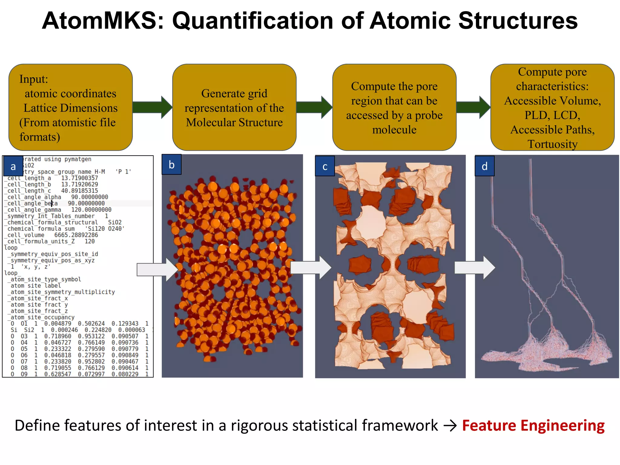
a c db
Input:
atomic coordinates
Lattice Dimensions
(From atomistic file
formats)
Generate grid
representation of the
Molecular Structure
Compute the pore
region that can be
accessed by a probe
molecule
Compute pore
characteristics:
Accessible Volume,
PLD, LCD,
Accessible Paths,
Tortuosity
AtomMKS: Quantification of Atomic Structures
Define features of interest in a rigorous statistical framework → Feature Engineering
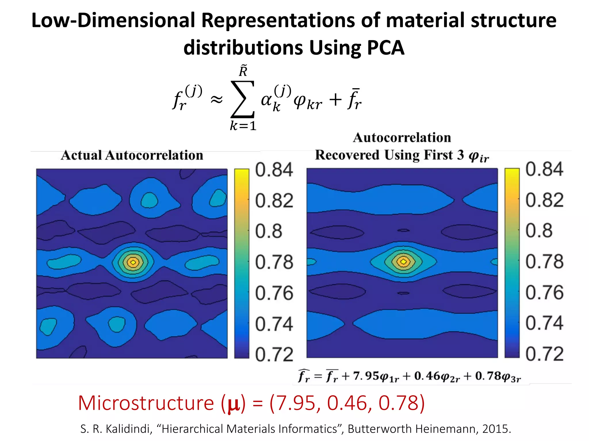
Low-Dimensional Representations of material structure
distributions Using PCA
𝑓𝑓𝑟𝑟
(𝑗𝑗)
≈ �
𝑘𝑘=1
�𝑅𝑅
𝛼𝛼𝑘𝑘
(𝑗𝑗)
𝜑𝜑𝑘𝑘𝑘𝑘 + ̅𝑓𝑓𝑟𝑟
Microstructure (µ) = (7.95, 0.46, 0.78)
S. R. Kalidindi, “Hierarchical Materials Informatics”, Butterworth Heinemann, 2015.
11
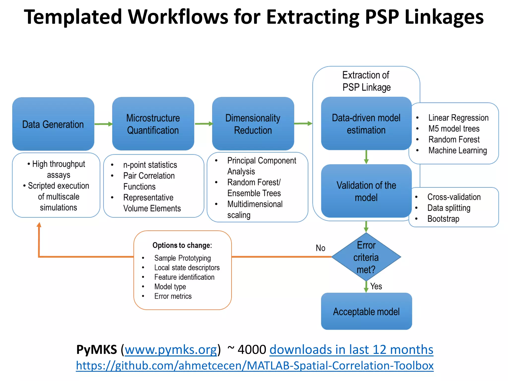
Templated Workflows for Extracting PSP Linkages
PyMKS (www.pymks.org) ~ 4000 downloads in last 12 months
https://github.com/ahmetcecen/MATLAB-Spatial-Correlation-Toolbox
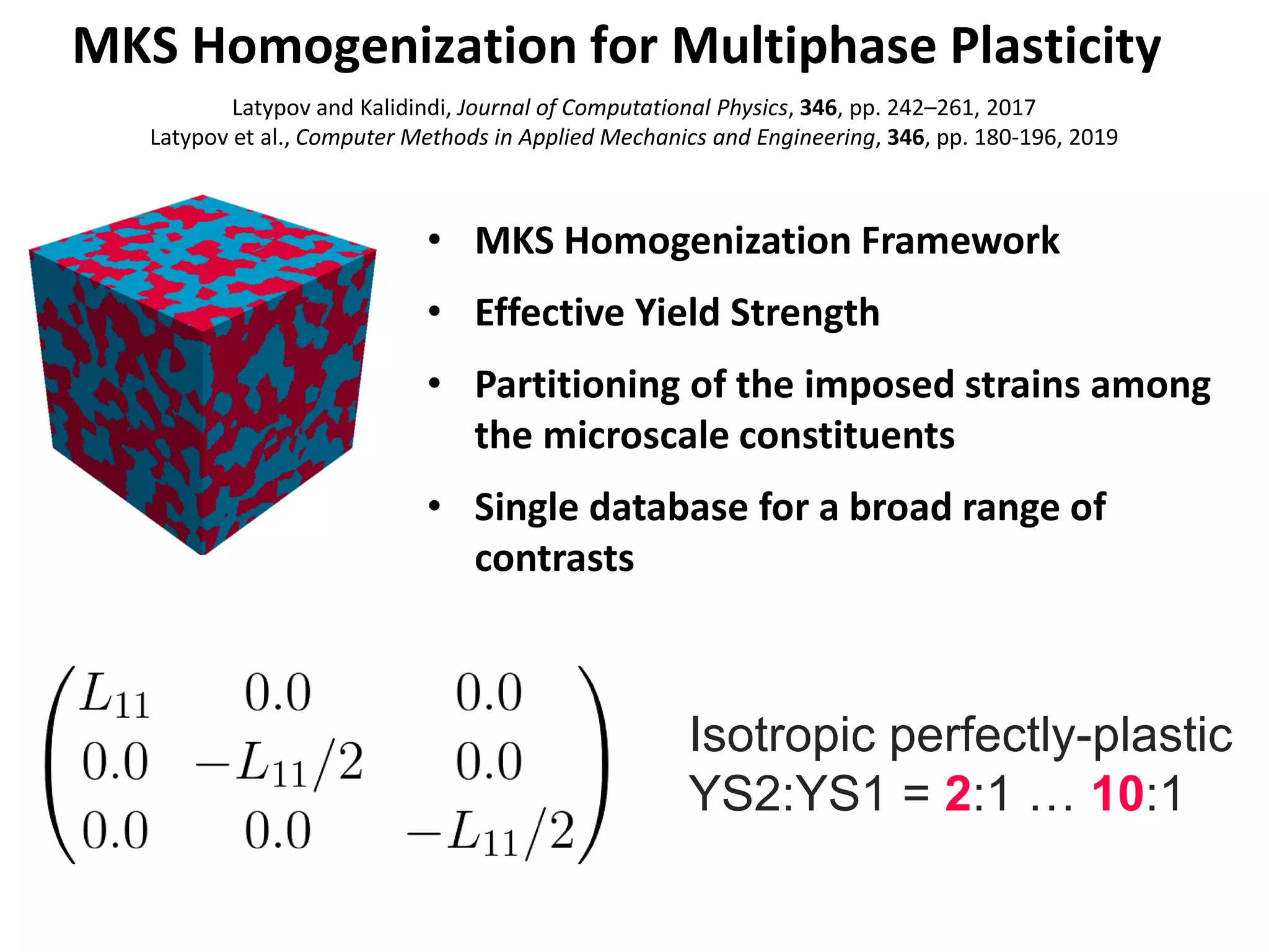
MKS Homogenization for Multiphase Plasticity
• MKS Homogenization Framework
• Effective Yield Strength
• Partitioning of the imposed strains among
the microscale constituents
• Single database for a broad range of
contrasts
Isotropic perfectly-plastic
YS2:YS1 = 2:1 … 10:1
Latypov and Kalidindi, Journal of Computational Physics, 346, pp. 242–261, 2017
Latypov et al., Computer Methods in Applied Mechanics and Engineering, 346, pp. 180-196, 2019
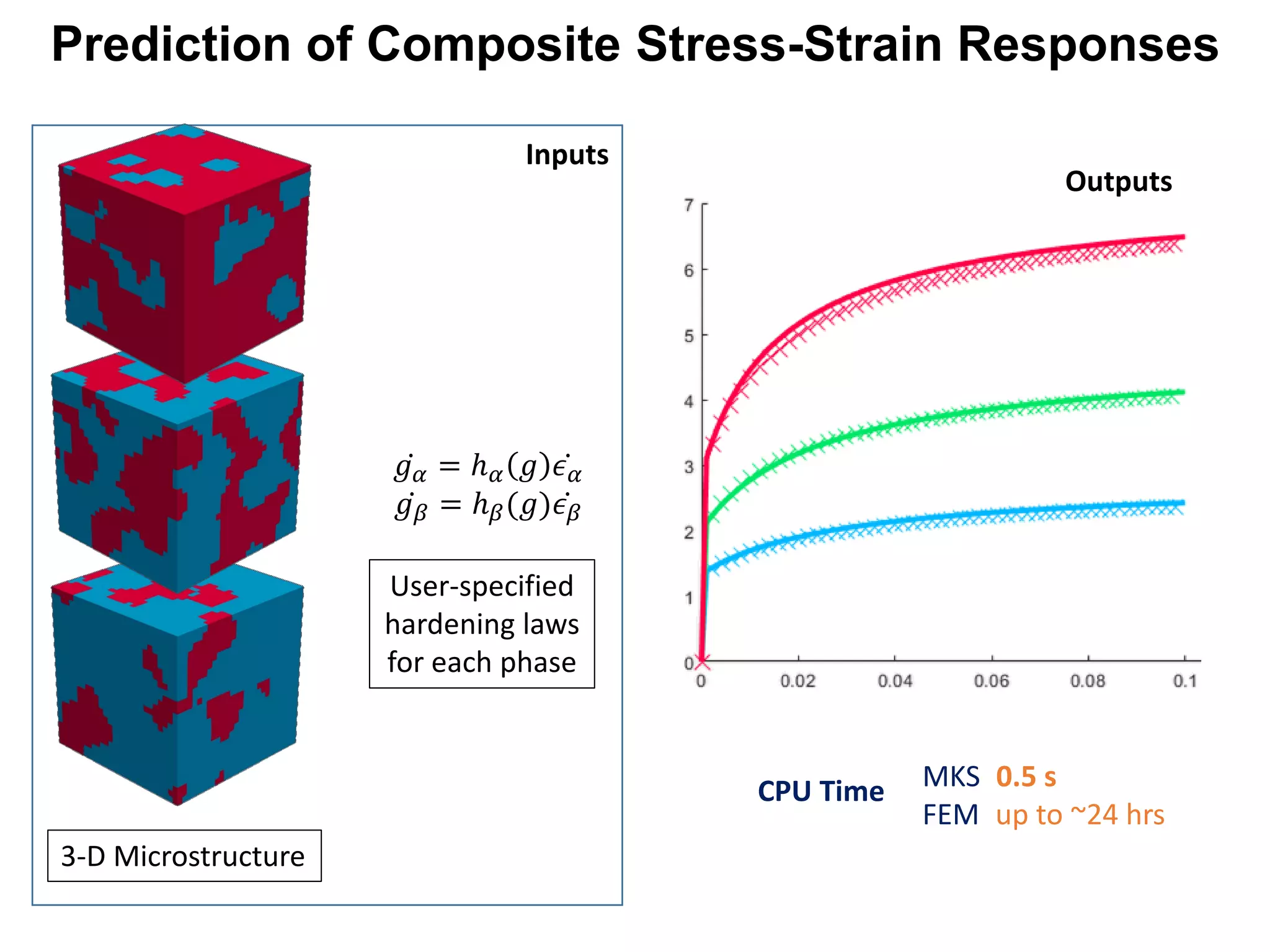
Prediction of Composite Stress-Strain Responses
FEM
MKS
User-specified
hardening laws
for each phase
̇𝑔𝑔𝛼𝛼 = ℎ𝛼𝛼 𝑔𝑔 ̇𝜖𝜖𝛼𝛼
̇𝑔𝑔𝛽𝛽 = ℎ𝛽𝛽(𝑔𝑔) ̇𝜖𝜖𝛽𝛽
3-D Microstructure
Inputs
CPU Time MKS: 0.5 s
FEM: up to ~24 hrs
Outputs
Correlation of Images to Properties
Optical Images of Steel Samples
500 550 600 650 700 750 800 850 900 950
Predicted Value
500
550
600
650
700
750
800
850
900
950
TrueYieldStrValue
𝐴𝐴𝐴𝐴𝐴𝐴𝐴𝐴𝐴𝐴𝐴𝐴𝐴𝐴 𝑒𝑒𝑒𝑒𝑒𝑒𝑒𝑒𝑒𝑒 = 2.5%
Image Segmentation Reduced-Order Microstructure
Representation
Reduced-Order Model
Grain 1
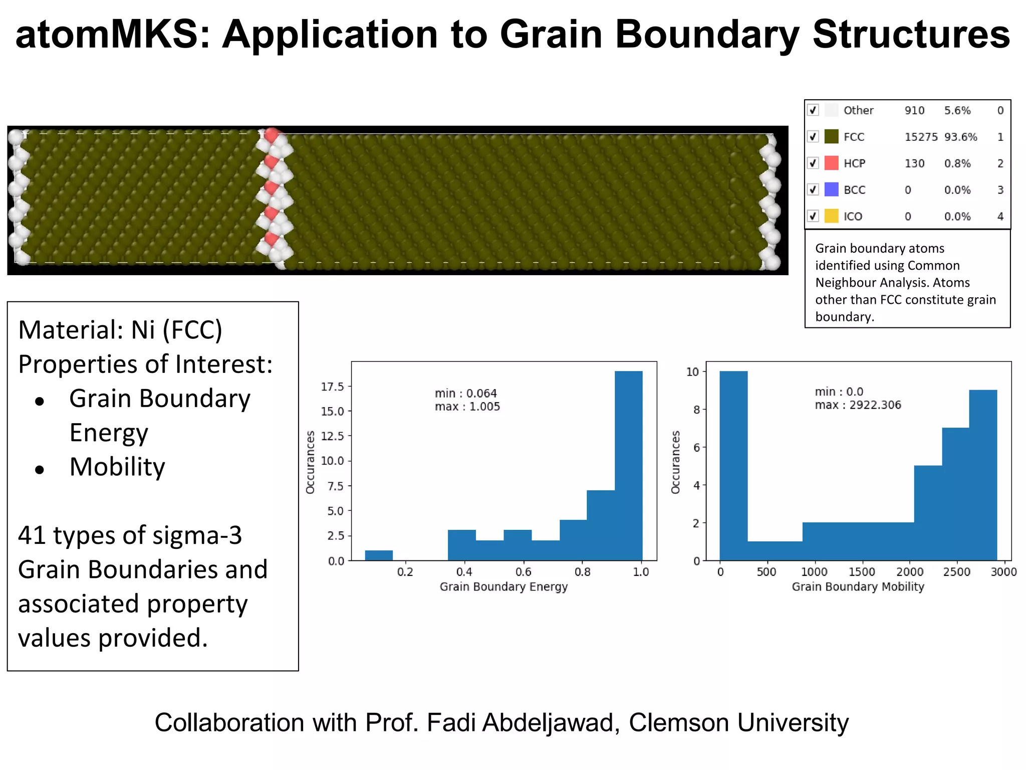
Material: Ni (FCC)
Properties of Interest:
● Grain Boundary
Energy
● Mobility
41 types of sigma-3
Grain Boundaries and
associated property
values provided.
Grain boundary atoms
identified using Common
Neighbour Analysis. Atoms
other than FCC constitute grain
boundary.
atomMKS: Application to Grain Boundary Structures
Collaboration with Prof. Fadi Abdeljawad, Clemson University
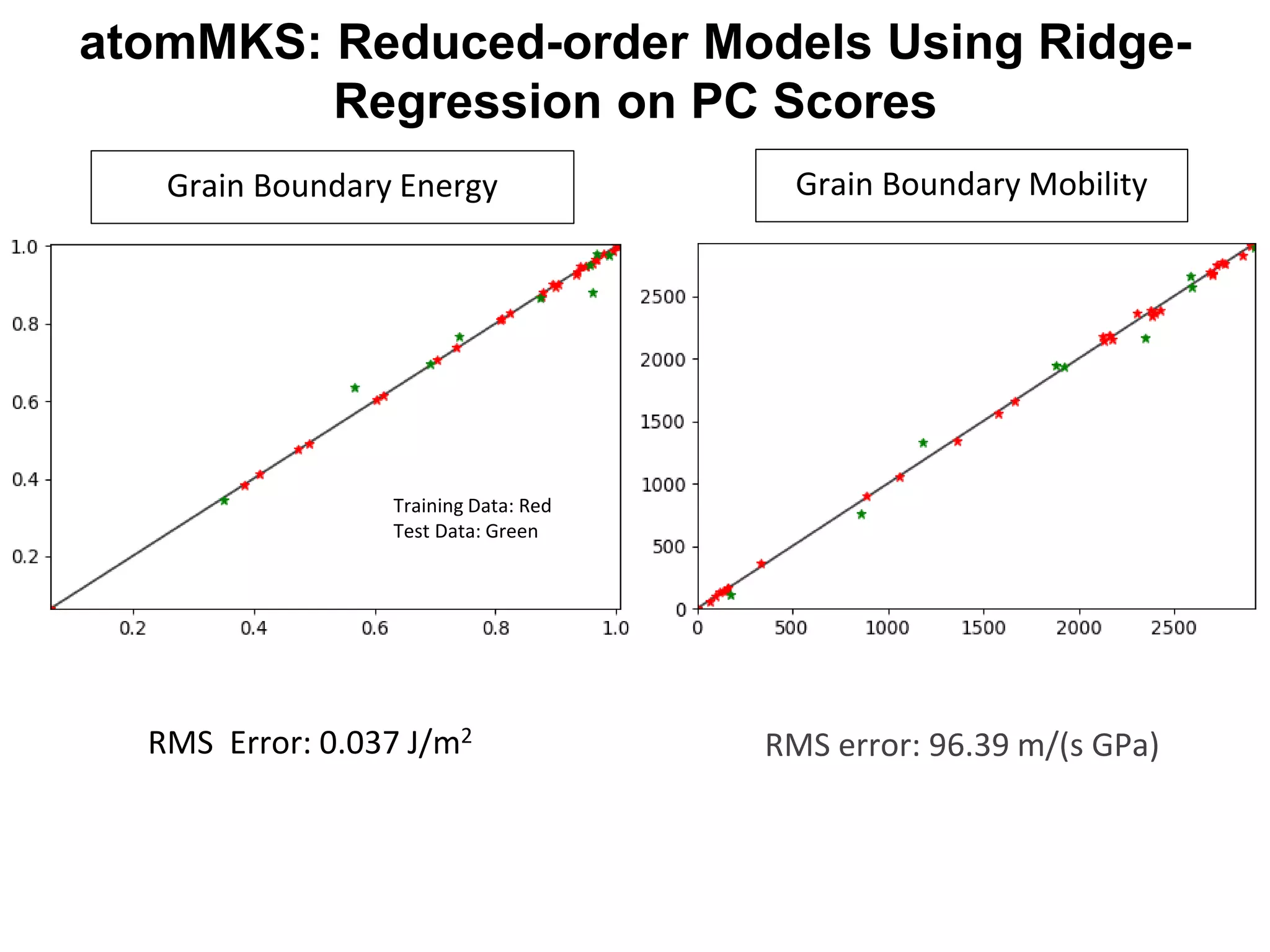
RMS Error: 0.037 J/m2
RMS error: 96.39 m/(s GPa)
Grain Boundary MobilityGrain Boundary Energy
Training Data: Red
Test Data: Green
atomMKS: Reduced-order Models Using Ridge-
Regression on PC Scores
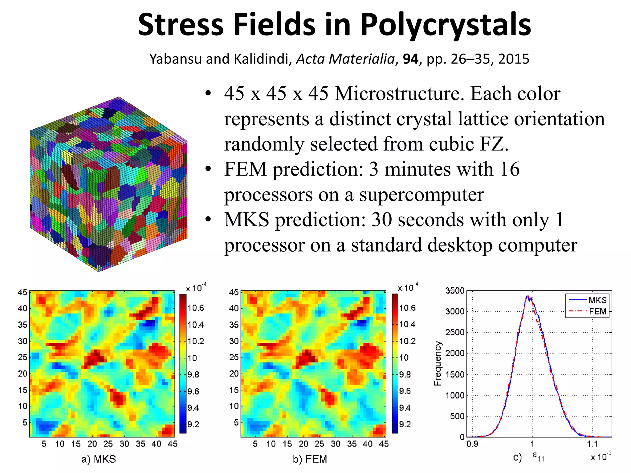
• 45 x 45 x 45 Microstructure. Each color
represents a distinct crystal lattice orientation
randomly selected from cubic FZ.
• FEM prediction: 3 minutes with 16
processors on a supercomputer
• MKS prediction: 30 seconds with only 1
processor on a standard desktop computer
Stress Fields in Polycrystals
Yabansu and Kalidindi, Acta Materialia, 94, pp. 26–35, 2015
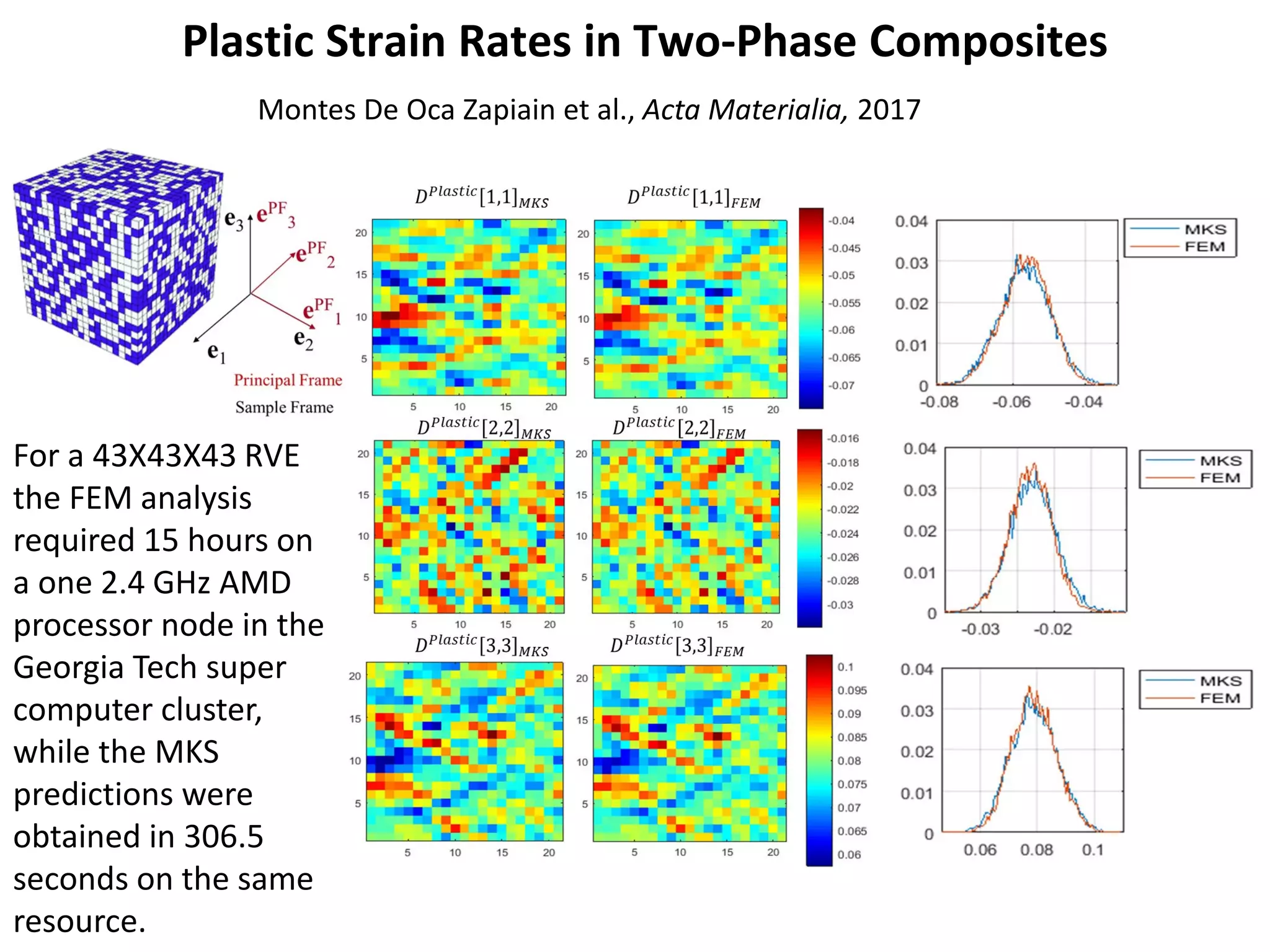
For a 43X43X43 RVE
the FEM analysis
required 15 hours on
a one 2.4 GHz AMD
processor node in the
Georgia Tech super
computer cluster,
while the MKS
predictions were
obtained in 306.5
seconds on the same
resource.
Plastic Strain Rates in Two-Phase Composites
Montes De Oca Zapiain et al., Acta Materialia, 2017
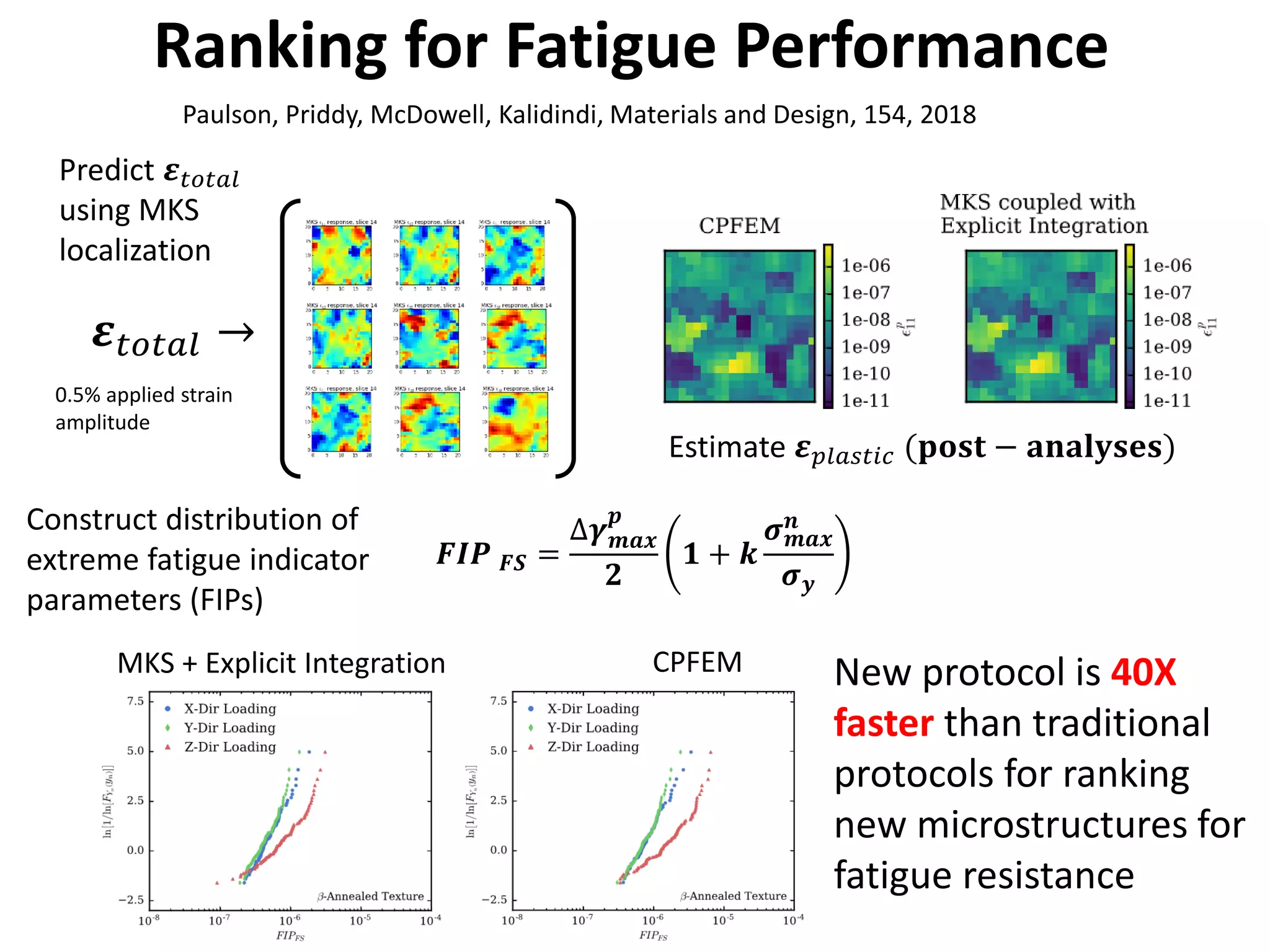
Ranking for Fatigue Performance
𝜺𝜺𝑡𝑡𝑡𝑡𝑡𝑡𝑎𝑎𝑎𝑎 →
0.5% applied strain
amplitude
MKS + Explicit Integration CPFEM
Predict 𝜺𝜺𝑡𝑡𝑡𝑡𝑡𝑡𝑎𝑎𝑎𝑎
using MKS
localization
Estimate 𝜺𝜺𝑝𝑝𝑝𝑝𝑝𝑝𝑝𝑝𝑝𝑝𝑝𝑝𝑝𝑝 (𝐩𝐩𝐩𝐩𝐩𝐩𝐩𝐩 − 𝐚𝐚𝐚𝐚𝐚𝐚𝐚𝐚𝐚𝐚𝐚𝐚𝐚𝐚𝐚𝐚)
Construct distribution of
extreme fatigue indicator
parameters (FIPs)
New protocol is 40X
faster than traditional
protocols for ranking
new microstructures for
fatigue resistance
𝑭𝑭𝑭𝑭𝑭𝑭 𝑭𝑭𝑭𝑭 =
∆𝜸𝜸 𝒎𝒎𝒎𝒎𝒎𝒎
𝒑𝒑
𝟐𝟐
𝟏𝟏 + 𝒌𝒌
𝝈𝝈 𝒎𝒎𝒎𝒎𝒎𝒎
𝒏𝒏
𝝈𝝈𝒚𝒚
Paulson, Priddy, McDowell, Kalidindi, Materials and Design, 154, 2018
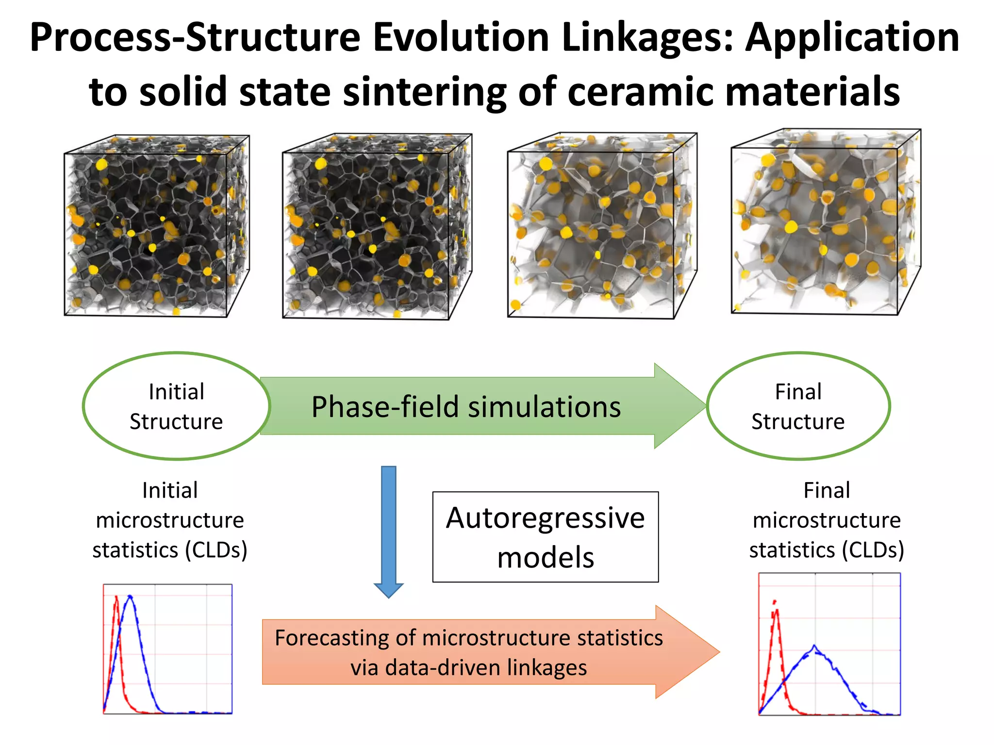
Forecasting of microstructure statistics
via data-driven linkages
Phase-field simulations
Initial
Structure
Final
Structure
Autoregressive
models
Initial
microstructure
statistics (CLDs)
Final
microstructure
statistics (CLDs)
Process-Structure Evolution Linkages: Application
to solid state sintering of ceramic materials
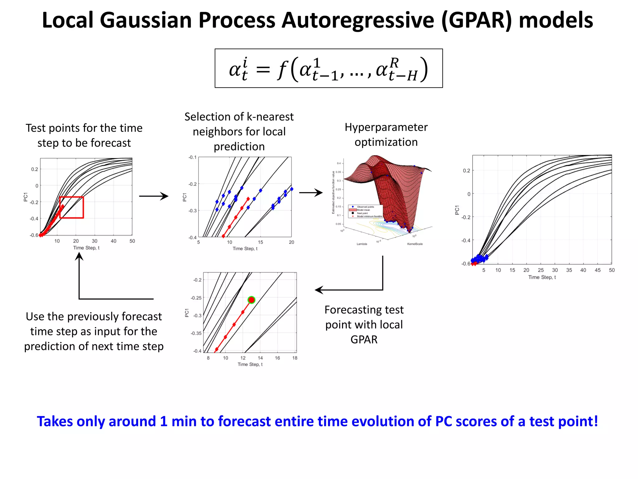
𝛼𝛼𝑡𝑡
𝑖𝑖
= 𝑓𝑓 𝛼𝛼𝑡𝑡−1
1
, … , 𝛼𝛼𝑡𝑡−𝐻𝐻
𝑅𝑅
Local Gaussian Process Autoregressive (GPAR) models
Hyperparameter
optimization
Test points for the time
step to be forecast
Selection of k-nearest
neighbors for local
prediction
Forecasting test
point with local
GPAR
Use the previously forecast
time step as input for the
prediction of next time step
Takes only around 1 min to forecast entire time evolution of PC scores of a test point!
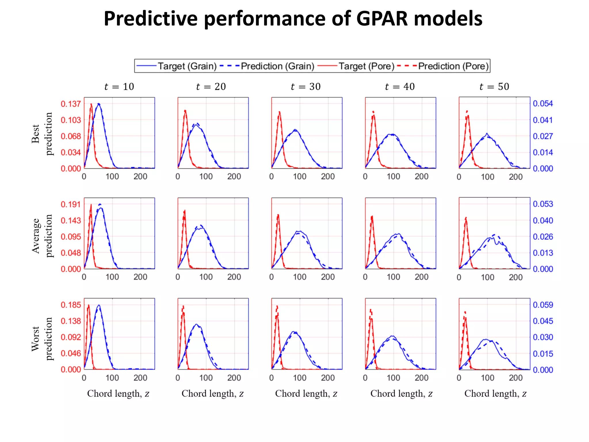
Predictive performance of GPAR models
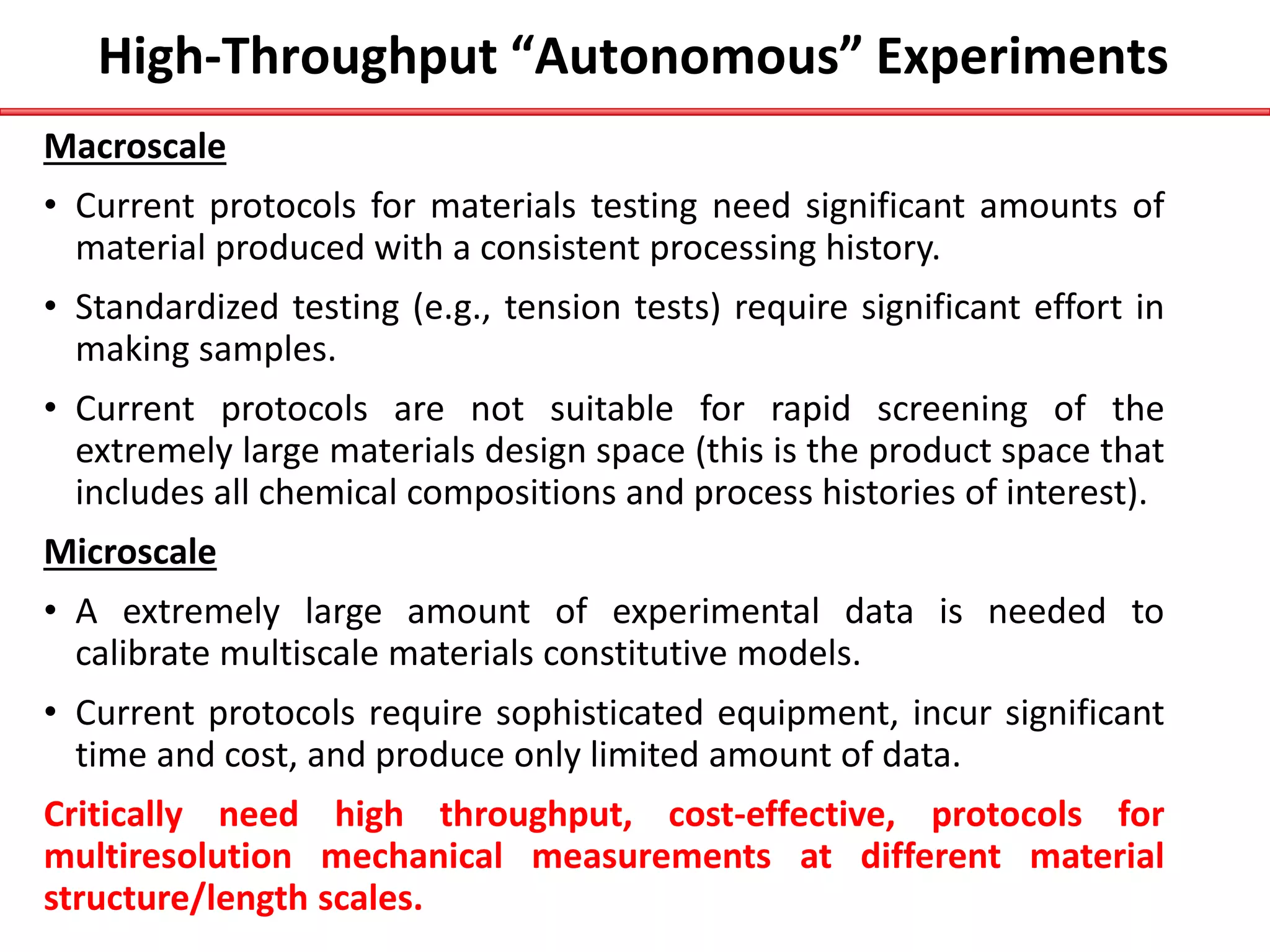
High-Throughput “Autonomous” Experiments
Macroscale
• Current protocols for materials testing need significant amounts of
material produced with a consistent processing history.
• Standardized testing (e.g., tension tests) require significant effort in
making samples.
• Current protocols are not suitable for rapid screening of the
extremely large materials design space (this is the product space that
includes all chemical compositions and process histories of interest).
Microscale
• A extremely large amount of experimental data is needed to
calibrate multiscale materials constitutive models.
• Current protocols require sophisticated equipment, incur significant
time and cost, and produce only limited amount of data.
Critically need high throughput, cost-effective, protocols for
multiresolution mechanical measurements at different material
structure/length scales.
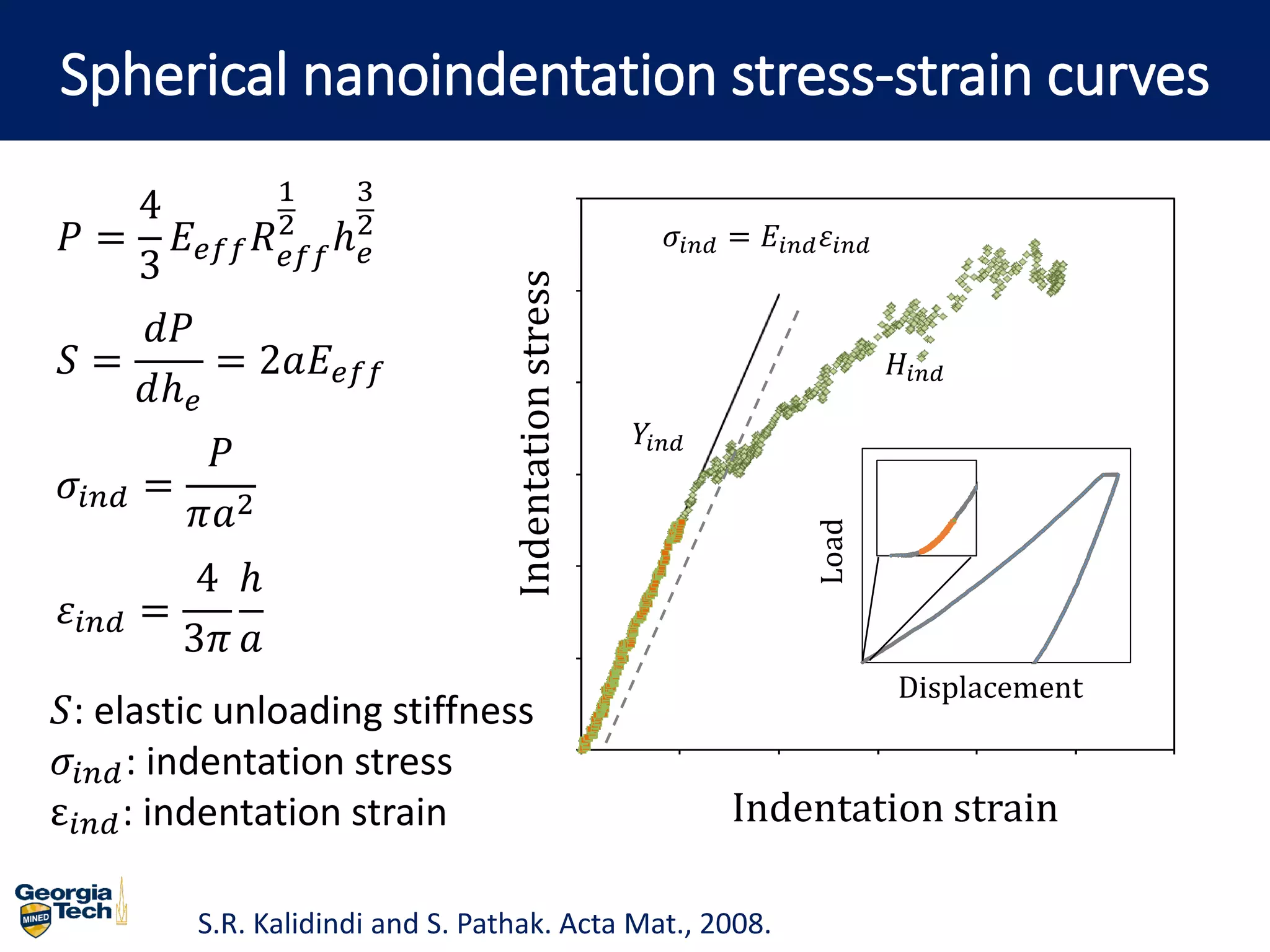
Spherical nanoindentation stress-strain curves
S.R. Kalidindi and S. Pathak. Acta Mat., 2008.
Indentation strain
Indentationstress
𝑌𝑌𝑖𝑖 𝑖𝑖 𝑖𝑖
𝜎𝜎𝑖𝑖 𝑖𝑖 𝑖𝑖 = 𝐸𝐸𝑖𝑖 𝑖𝑖 𝑖𝑖 𝜀𝜀𝑖𝑖 𝑖𝑖 𝑖𝑖
Load
Displacement
𝐻𝐻𝑖𝑖 𝑖𝑖 𝑖𝑖
𝜎𝜎𝑖𝑖 𝑖𝑖 𝑖𝑖 =
𝑃𝑃
𝜋𝜋𝑎𝑎2
𝜀𝜀𝑖𝑖 𝑖𝑖 𝑖𝑖 =
4
3𝜋𝜋
ℎ
𝑎𝑎
𝑆𝑆 =
𝑑𝑑𝑑𝑑
𝑑𝑑ℎ𝑒𝑒
= 2𝑎𝑎𝐸𝐸𝑒𝑒𝑒𝑒𝑒𝑒
𝑃𝑃 =
4
3
𝐸𝐸𝑒𝑒𝑒𝑒𝑒𝑒 𝑅𝑅𝑒𝑒𝑒𝑒𝑒𝑒
1
2
ℎ𝑒𝑒
3
2
𝑆𝑆: elastic unloading stiffness
𝜎𝜎𝑖𝑖 𝑖𝑖 𝑖𝑖: indentation stress
ε𝑖𝑖 𝑖𝑖 𝑖𝑖: indentation strain
Applications to Rapid Screening of Process Space
0
100
200
300
400
500
600
700
200 300 400IndentationStrength[MPa]
Aging Temperature [°C]
High Throughput Sample
Individual Heat Treatments
0
100
200
300
400
500
600
700
AR 204 °C 274 °C 343 °C 413 °C
Strength[MPa]
Indentation Yield Strength
Tensile Yield Strength
Orientation Dependence of
Indentation Properties of primary α
in Ti alloys
60
80
100
120
140
160
180
0 20 40 60 80 100
Indentationmodulus[GPa]
Declination angle
Indentation Modulus, MPa
Primary α
Ti64
Ti5-2.5
Ti811
Ti6242
0
0.5
1
1.5
2
2.5
3
3.5
4
4.5
0 20 40 60 80 100
IndentationYieldstrength[GPa]
Declination angle
Indentation Yield Strength, GPa
Primary α
Ti64
Ti5-2.5
Ti811
Ti6242
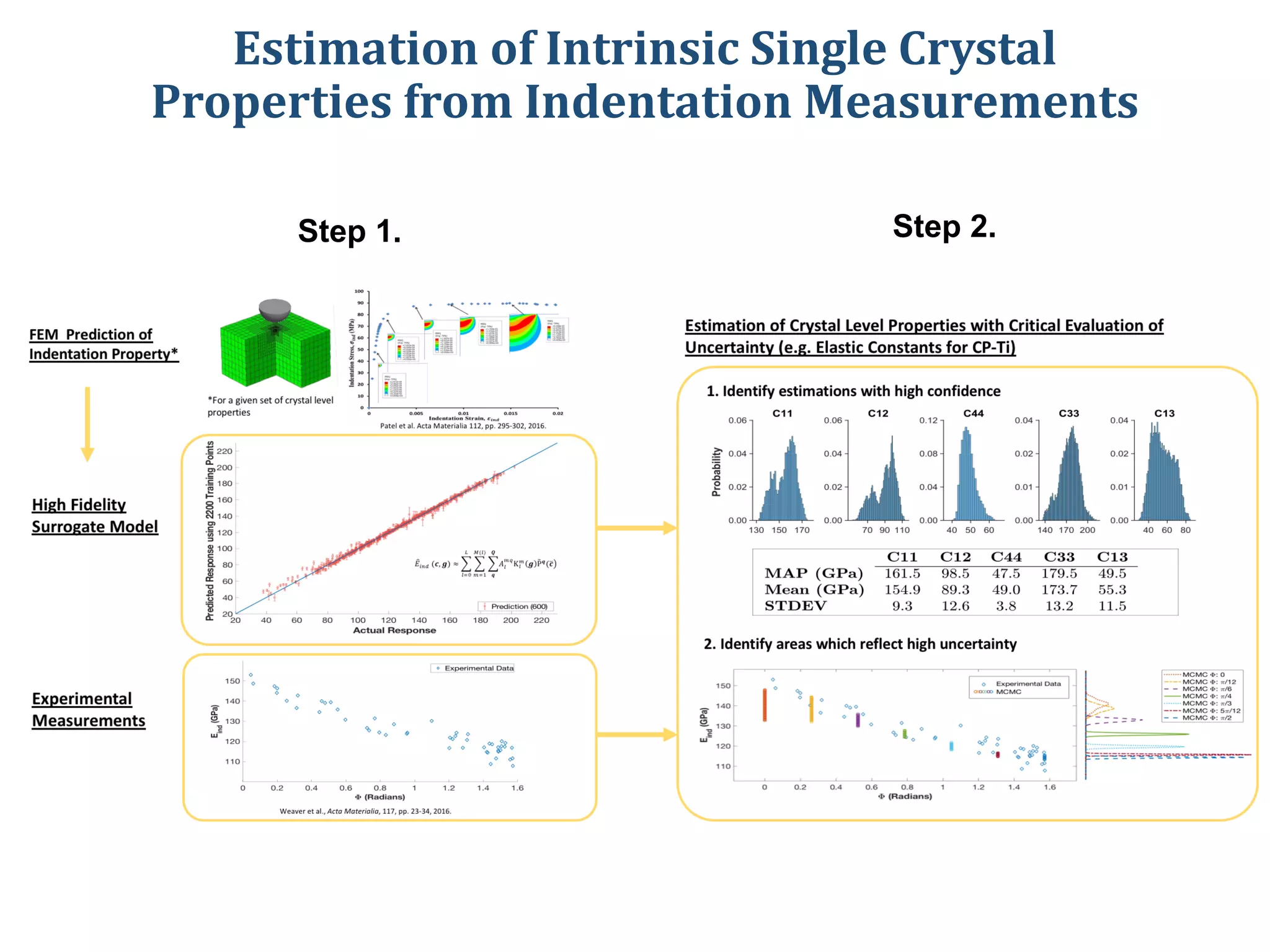
Estimation of Intrinsic Single Crystal
Properties from Indentation Measurements
Step 1. Step 2.
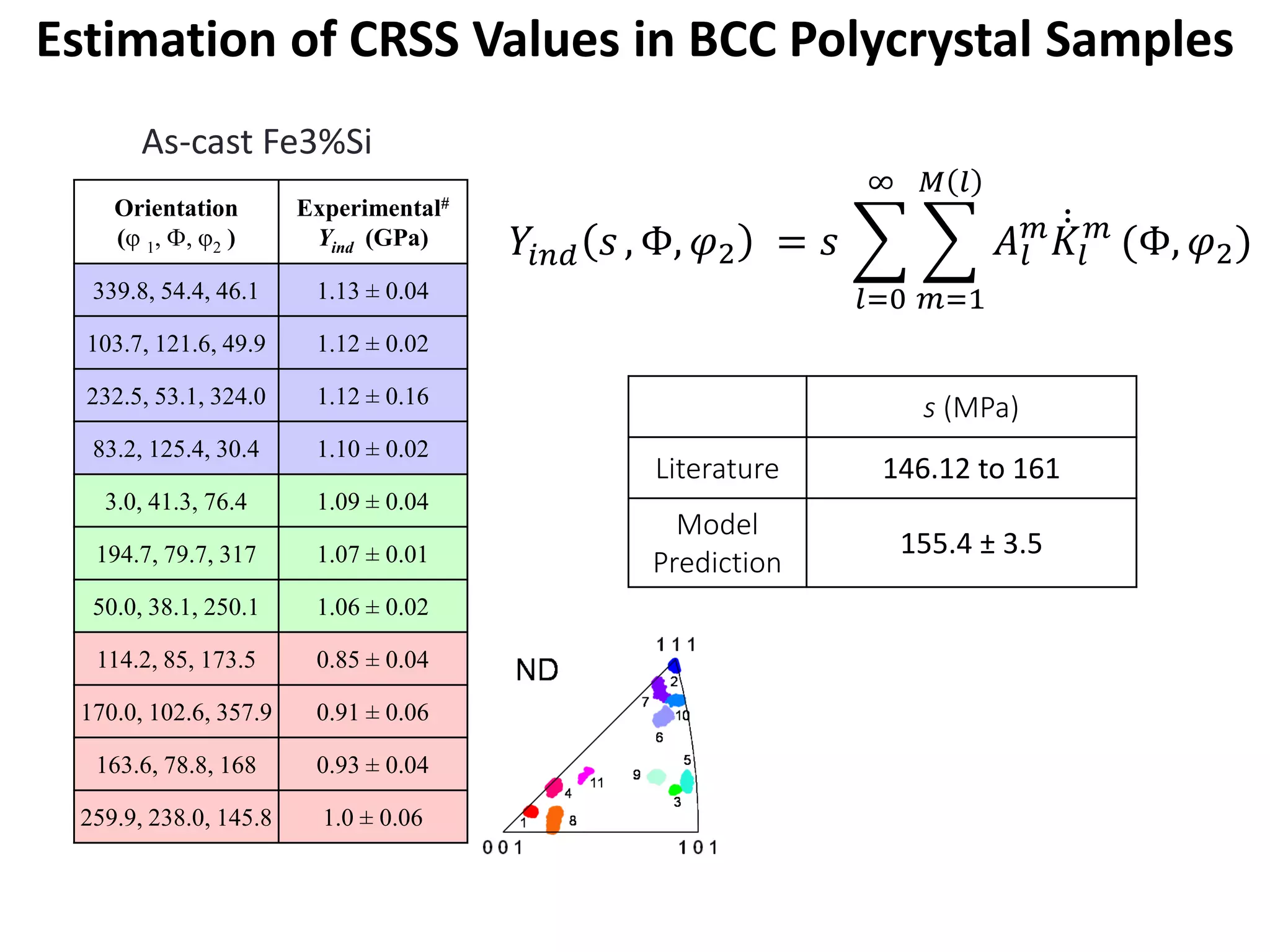
s (MPa)
Literature 146.12 to 161
Model
Prediction
155.4 ± 3.5
As-cast Fe3%Si
Orientation
(ϕ 1, Φ, ϕ2 )
Experimental#
Yind (GPa)
339.8, 54.4, 46.1 1.13 ± 0.04
103.7, 121.6, 49.9 1.12 ± 0.02
232.5, 53.1, 324.0 1.12 ± 0.16
83.2, 125.4, 30.4 1.10 ± 0.02
3.0, 41.3, 76.4 1.09 ± 0.04
194.7, 79.7, 317 1.07 ± 0.01
50.0, 38.1, 250.1 1.06 ± 0.02
114.2, 85, 173.5 0.85 ± 0.04
170.0, 102.6, 357.9 0.91 ± 0.06
163.6, 78.8, 168 0.93 ± 0.04
259.9, 238.0, 145.8 1.0 ± 0.06
𝑌𝑌𝑖𝑖 𝑖𝑖 𝑖𝑖 𝑠𝑠 , Φ, 𝜑𝜑2 = 𝑠𝑠 �
𝑙𝑙=0
∞
�
𝑚𝑚=1
𝑀𝑀 𝑙𝑙
𝐴𝐴𝑙𝑙
𝑚𝑚 ̇̇𝐾𝐾𝑙𝑙
𝑚𝑚
(Φ, 𝜑𝜑2)
Estimation of CRSS Values in BCC Polycrystal Samples
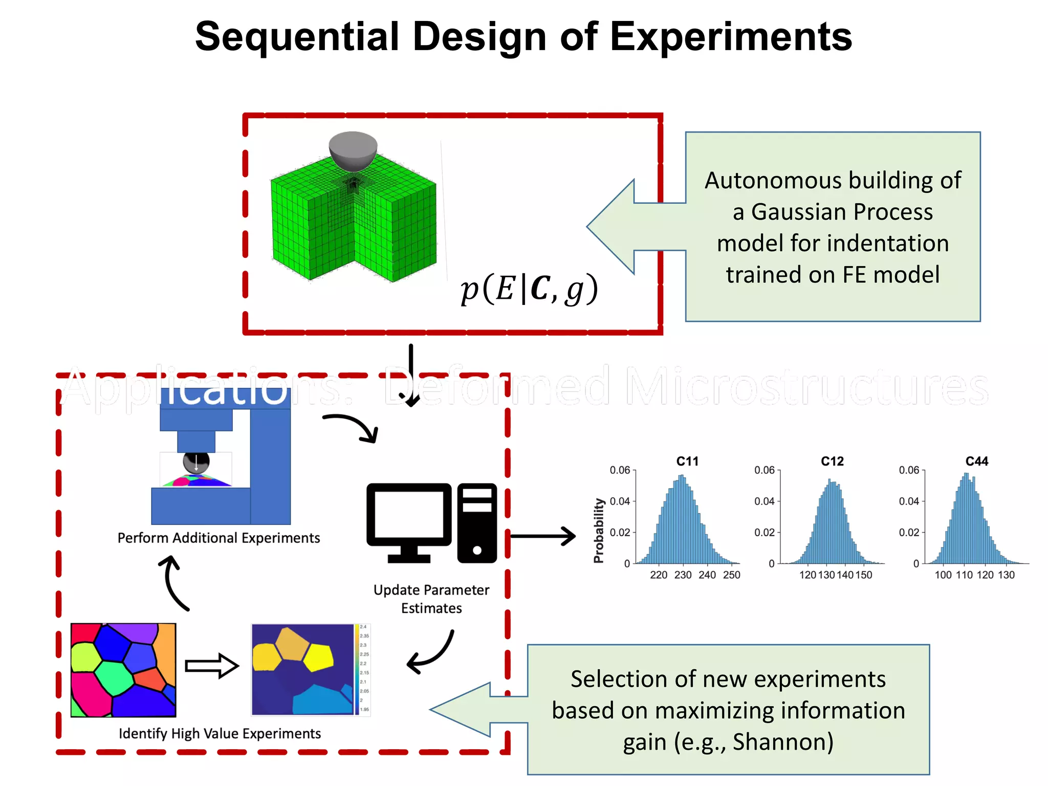
𝑝𝑝 𝐸𝐸 𝑪𝑪, 𝑔𝑔
Sequential Design of Experiments
Autonomous building of
a Gaussian Process
model for indentation
trained on FE model
Selection of new experiments
based on maximizing information
gain (e.g., Shannon)
• A physics-centered Bayesian framework can
serve as a foundational element in the design
and build of AI-based materials knowledge
systems that can provide objective decision
support in all aspects of materials innovation.
• High-throughput experimental and
computational protocols are critically needed
to generate the data needed to feed the
envisioned knowledge systems.
Summary Statements

A Machine Learning Framework for Materials Knowledge Systems

  • 1.
    A Machine LearningFramework for Materials Knowledge Systems Surya R. Kalidindi Funding: DoD, NIST
  • 2.
    AI-Based Materials KnowledgeSystems (MKS) Knowledge System PREDICT DIAGNOSE RECOMMEND • Specifically designed to support accelerated discovery, development, and deployment of new/improved materials in advanced technologies • Main Functions: Diagnose, Predict, Recommend • Expressed as a library of Process-Structure-Property (PSP) linkages covering all materials classes and all relevant material structure length scales (and relevant time scales) • Formulated on a rigorous Bayesian statistical framework that accounts for the uncertainty of the curated knowledge • Continuously ingests a variety of information from disparate sources and dynamically evolves • Highly efficient both in front-end (user-facing) and in the back-end (knowledge update) computations
  • 3.
    Process • Thermo- mechanical (T(t), L(t),σ(t), ̇𝑐𝑐(t), … ) • Placement of Specific Defects (e.g., grain/phase boundaries, 𝑔𝑔, ∆𝑔𝑔, 𝑛𝑛) • Placement of chemical species (𝑐𝑐𝑖𝑖, 𝑉𝑉, 𝑝𝑝, 𝒙𝒙𝑛𝑛, … ) Structure • Microstructure • Dislocation/defect structure • Interface atomic structure • Atomic structure with defects, disorder, etc. • Electron density field Property • Young’s Modulus • Yield Strength • Fatigue Strength • Conductivity • Permeability • Critical Resolved Shear Strength • Grain Boundary Energy • Vacancy Formation Energy PSP Linkages Over a Hierarchy of Material Structure Scales • Process and Property variables have rigorous mathematical definitions • Critical Need: A framework for high-value low-dimensional representations of the material structure (minimal information loss with maximum recoverability) that is broadly applicable to various material classes at different length scales.
  • 4.
    AI-Based Materials KnowledgeSystems (knowledge integration as opposed to tool integration) www.comsol.com DESIGN & MANUFACTURING P-S-P P-S-P P-S-P Major Classes of Information Sources • Experiments • Simulations
  • 5.
    Stochastic Framework forMKS • Property: 𝑃𝑃 ∈ ℛ; 𝑝𝑝 𝑃𝑃 = 𝒩𝒩 𝑃𝑃 �𝑃𝑃, 𝜎𝜎𝑝𝑝 2 • Material (Hierarchical) Structure: 𝝁𝝁 ∈ 𝓜𝓜; 𝑝𝑝 𝝁𝝁 = 𝒩𝒩 𝝁𝝁 �𝝁𝝁, 𝜮𝜮𝝁𝝁 • Process: 𝓟𝓟 ∈ ℛ𝑛𝑛 ; 𝑝𝑝 𝓟𝓟 = 𝒩𝒩 𝓟𝓟 �𝓟𝓟, 𝜮𝜮𝓟𝓟 • Governing Physics: expressed as field (differential) equations and material constitutive laws or equivalently as Green’s functions 𝝋𝝋 ∈ 𝚽𝚽; 𝑝𝑝 𝝋𝝋 = 𝒩𝒩 𝝋𝝋 �𝝋𝝋, 𝜮𝜮𝝋𝝋 • Physics-Based Simulations: 𝑝𝑝 𝑃𝑃 𝝁𝝁, 𝝋𝝋, 𝜮𝜮𝝁𝝁 , 𝜮𝜮𝝋𝝋 and 𝑝𝑝 𝝁𝝁 𝓟𝓟, 𝝋𝝋, 𝜮𝜮𝓟𝓟 , 𝜮𝜮𝝋𝝋 - machine learning has opened new avenues for sampling these distributions within practical computational budgets • Physical Experiments (typically small datasets): 𝑝𝑝 𝑃𝑃 𝝁𝝁, 𝜮𝜮𝝁𝝁 , 𝝋𝝋∗ and 𝑝𝑝 𝝁𝝁 𝓟𝓟, 𝜮𝜮𝓟𝓟 , 𝝋𝝋∗ ; 𝝋𝝋∗ = undetermined governing physics
  • 6.
    Bayesian Update ofGoverning Physics (a formal framework for uncovering new physics) 𝑝𝑝 𝝋𝝋 𝑬𝑬, 𝜮𝜮𝑬𝑬 ∝ 𝑝𝑝 𝑬𝑬 𝝋𝝋, 𝜮𝜮𝑬𝑬 𝑝𝑝 𝝋𝝋 Physics-Based Simulations Build Gaussian Process models trained to simulation datasets produced by executing physics-based models by adaptive sampling of input domain for maximizing fidelity of extracted GP. Process-Structure: 𝑝𝑝 𝝁𝝁 𝓟𝓟, 𝝋𝝋, 𝜮𝜮𝓟𝓟 , 𝜮𝜮𝝋𝝋 Structure-Property: 𝑝𝑝 𝑃𝑃 𝝁𝝁, 𝝋𝝋, 𝜮𝜮𝝁𝝁 , 𝜮𝜮𝝋𝝋 Sequential Design of Physical Experiments Decide on the next experiment that is likely to produce the largest information gain in updating the governing physics. Foundational framework for Materials Knowledge Systems: Diagnose, Predict, Recommend
  • 7.
    Structure Quantification: n-PointSpatial Correlations • Spatial correlations capture all of the salient measures of the microstructure • Allow efficient computations using discrete Fourier transforms (DFTs) 𝑓𝑓𝒓𝒓 𝑛𝑛𝑛𝑛 = 1 𝑆𝑆𝒓𝒓 1 𝐽𝐽 � 𝒔𝒔 � 𝑗𝑗=1 𝐽𝐽 (𝑗𝑗) 𝑚𝑚𝒔𝒔 𝑛𝑛 (𝑗𝑗) 𝑚𝑚𝒔𝒔+𝒓𝒓 𝑝𝑝 𝑓𝑓𝑟𝑟 ℎℎ′ = # 𝑇𝑇𝑇𝑇𝑇𝑇𝑇𝑇𝑇𝑇𝑇𝑇 𝑆𝑆𝑆𝑆𝑆𝑆𝑆𝑆𝑆𝑆𝑆𝑆𝑆𝑆𝑆𝑆𝑆𝑆𝑆𝑆 # 𝑇𝑇𝑇𝑇𝑇𝑇𝑇𝑇𝑇𝑇𝑇𝑇 𝐴𝐴𝐴𝐴𝐴𝐴 𝐴𝐴𝐴𝐴𝐴𝐴𝐴𝐴𝐴𝐴𝐴𝐴 %50 %0 Complete Set of 𝑓𝑓𝑟𝑟 ℎℎ′ for all possible 𝑟𝑟 S. R. Kalidindi, “Hierarchical Materials Informatics”, Butterworth Heinemann, 2015.
  • 8.
    Polycrystal Microstructures 𝑚𝑚 𝑔𝑔,𝒙𝒙 ≈ � 𝐿𝐿 �𝐿𝐿 � 𝒔𝒔 𝑺𝑺 𝑀𝑀𝒔𝒔 𝐿𝐿 𝑇𝑇𝐿𝐿 𝑔𝑔 𝜒𝜒𝒔𝒔 𝒙𝒙 𝑓𝑓 𝑔𝑔, 𝑔𝑔𝑔 𝒓𝒓 ≈ � 𝐿𝐿 �𝐿𝐿 � 𝐾𝐾 �𝐿𝐿 � 𝒕𝒕 𝑺𝑺 𝐹𝐹𝒕𝒕 𝐿𝐿𝐿𝐿 𝑇𝑇𝐿𝐿 𝑔𝑔 𝑇𝑇𝐾𝐾 𝑔𝑔𝑔 𝜒𝜒𝒕𝒕 𝒓𝒓 𝑓𝑓 𝑔𝑔, 𝑔𝑔𝑔 𝒓𝒓 = 1 𝑉𝑉𝑉𝑉𝑉𝑉(Ω𝒓𝒓) � Ω𝒓𝒓 𝑚𝑚 𝑔𝑔, 𝒙𝒙 𝑚𝑚 𝑔𝑔′, 𝒙𝒙 + 𝒓𝒓 𝑑𝑑𝒙𝒙 𝐹𝐹𝒕𝒕 𝐿𝐿𝐿𝐿 = 1 𝑺𝑺𝒕𝒕 � 𝒔𝒔 𝑺𝑺𝒕𝒕 𝑴𝑴𝒔𝒔 𝐿𝐿 𝑴𝑴𝒔𝒔+𝒕𝒕 𝐾𝐾
  • 9.
    a c db Input: atomiccoordinates Lattice Dimensions (From atomistic file formats) Generate grid representation of the Molecular Structure Compute the pore region that can be accessed by a probe molecule Compute pore characteristics: Accessible Volume, PLD, LCD, Accessible Paths, Tortuosity AtomMKS: Quantification of Atomic Structures Define features of interest in a rigorous statistical framework → Feature Engineering
  • 10.
    Low-Dimensional Representations ofmaterial structure distributions Using PCA 𝑓𝑓𝑟𝑟 (𝑗𝑗) ≈ � 𝑘𝑘=1 �𝑅𝑅 𝛼𝛼𝑘𝑘 (𝑗𝑗) 𝜑𝜑𝑘𝑘𝑘𝑘 + ̅𝑓𝑓𝑟𝑟 Microstructure (µ) = (7.95, 0.46, 0.78) S. R. Kalidindi, “Hierarchical Materials Informatics”, Butterworth Heinemann, 2015.
  • 11.
    11 Templated Workflows forExtracting PSP Linkages PyMKS (www.pymks.org) ~ 4000 downloads in last 12 months https://github.com/ahmetcecen/MATLAB-Spatial-Correlation-Toolbox
  • 12.
    MKS Homogenization forMultiphase Plasticity • MKS Homogenization Framework • Effective Yield Strength • Partitioning of the imposed strains among the microscale constituents • Single database for a broad range of contrasts Isotropic perfectly-plastic YS2:YS1 = 2:1 … 10:1 Latypov and Kalidindi, Journal of Computational Physics, 346, pp. 242–261, 2017 Latypov et al., Computer Methods in Applied Mechanics and Engineering, 346, pp. 180-196, 2019
  • 13.
    Prediction of CompositeStress-Strain Responses FEM MKS User-specified hardening laws for each phase ̇𝑔𝑔𝛼𝛼 = ℎ𝛼𝛼 𝑔𝑔 ̇𝜖𝜖𝛼𝛼 ̇𝑔𝑔𝛽𝛽 = ℎ𝛽𝛽(𝑔𝑔) ̇𝜖𝜖𝛽𝛽 3-D Microstructure Inputs CPU Time MKS: 0.5 s FEM: up to ~24 hrs Outputs
  • 14.
    Correlation of Imagesto Properties Optical Images of Steel Samples 500 550 600 650 700 750 800 850 900 950 Predicted Value 500 550 600 650 700 750 800 850 900 950 TrueYieldStrValue 𝐴𝐴𝐴𝐴𝐴𝐴𝐴𝐴𝐴𝐴𝐴𝐴𝐴𝐴 𝑒𝑒𝑒𝑒𝑒𝑒𝑒𝑒𝑒𝑒 = 2.5% Image Segmentation Reduced-Order Microstructure Representation Reduced-Order Model
  • 15.
    Grain 1 Material: Ni(FCC) Properties of Interest: ● Grain Boundary Energy ● Mobility 41 types of sigma-3 Grain Boundaries and associated property values provided. Grain boundary atoms identified using Common Neighbour Analysis. Atoms other than FCC constitute grain boundary. atomMKS: Application to Grain Boundary Structures Collaboration with Prof. Fadi Abdeljawad, Clemson University
  • 16.
    RMS Error: 0.037J/m2 RMS error: 96.39 m/(s GPa) Grain Boundary MobilityGrain Boundary Energy Training Data: Red Test Data: Green atomMKS: Reduced-order Models Using Ridge- Regression on PC Scores
  • 17.
    • 45 x45 x 45 Microstructure. Each color represents a distinct crystal lattice orientation randomly selected from cubic FZ. • FEM prediction: 3 minutes with 16 processors on a supercomputer • MKS prediction: 30 seconds with only 1 processor on a standard desktop computer Stress Fields in Polycrystals Yabansu and Kalidindi, Acta Materialia, 94, pp. 26–35, 2015
  • 18.
    For a 43X43X43RVE the FEM analysis required 15 hours on a one 2.4 GHz AMD processor node in the Georgia Tech super computer cluster, while the MKS predictions were obtained in 306.5 seconds on the same resource. Plastic Strain Rates in Two-Phase Composites Montes De Oca Zapiain et al., Acta Materialia, 2017
  • 19.
    Ranking for FatiguePerformance 𝜺𝜺𝑡𝑡𝑡𝑡𝑡𝑡𝑎𝑎𝑎𝑎 → 0.5% applied strain amplitude MKS + Explicit Integration CPFEM Predict 𝜺𝜺𝑡𝑡𝑡𝑡𝑡𝑡𝑎𝑎𝑎𝑎 using MKS localization Estimate 𝜺𝜺𝑝𝑝𝑝𝑝𝑝𝑝𝑝𝑝𝑝𝑝𝑝𝑝𝑝𝑝 (𝐩𝐩𝐩𝐩𝐩𝐩𝐩𝐩 − 𝐚𝐚𝐚𝐚𝐚𝐚𝐚𝐚𝐚𝐚𝐚𝐚𝐚𝐚𝐚𝐚) Construct distribution of extreme fatigue indicator parameters (FIPs) New protocol is 40X faster than traditional protocols for ranking new microstructures for fatigue resistance 𝑭𝑭𝑭𝑭𝑭𝑭 𝑭𝑭𝑭𝑭 = ∆𝜸𝜸 𝒎𝒎𝒎𝒎𝒎𝒎 𝒑𝒑 𝟐𝟐 𝟏𝟏 + 𝒌𝒌 𝝈𝝈 𝒎𝒎𝒎𝒎𝒎𝒎 𝒏𝒏 𝝈𝝈𝒚𝒚 Paulson, Priddy, McDowell, Kalidindi, Materials and Design, 154, 2018
  • 20.
    Forecasting of microstructurestatistics via data-driven linkages Phase-field simulations Initial Structure Final Structure Autoregressive models Initial microstructure statistics (CLDs) Final microstructure statistics (CLDs) Process-Structure Evolution Linkages: Application to solid state sintering of ceramic materials
  • 21.
    𝛼𝛼𝑡𝑡 𝑖𝑖 = 𝑓𝑓 𝛼𝛼𝑡𝑡−1 1 ,… , 𝛼𝛼𝑡𝑡−𝐻𝐻 𝑅𝑅 Local Gaussian Process Autoregressive (GPAR) models Hyperparameter optimization Test points for the time step to be forecast Selection of k-nearest neighbors for local prediction Forecasting test point with local GPAR Use the previously forecast time step as input for the prediction of next time step Takes only around 1 min to forecast entire time evolution of PC scores of a test point!
  • 22.
  • 23.
    High-Throughput “Autonomous” Experiments Macroscale •Current protocols for materials testing need significant amounts of material produced with a consistent processing history. • Standardized testing (e.g., tension tests) require significant effort in making samples. • Current protocols are not suitable for rapid screening of the extremely large materials design space (this is the product space that includes all chemical compositions and process histories of interest). Microscale • A extremely large amount of experimental data is needed to calibrate multiscale materials constitutive models. • Current protocols require sophisticated equipment, incur significant time and cost, and produce only limited amount of data. Critically need high throughput, cost-effective, protocols for multiresolution mechanical measurements at different material structure/length scales.
  • 24.
    Spherical nanoindentation stress-straincurves S.R. Kalidindi and S. Pathak. Acta Mat., 2008. Indentation strain Indentationstress 𝑌𝑌𝑖𝑖 𝑖𝑖 𝑖𝑖 𝜎𝜎𝑖𝑖 𝑖𝑖 𝑖𝑖 = 𝐸𝐸𝑖𝑖 𝑖𝑖 𝑖𝑖 𝜀𝜀𝑖𝑖 𝑖𝑖 𝑖𝑖 Load Displacement 𝐻𝐻𝑖𝑖 𝑖𝑖 𝑖𝑖 𝜎𝜎𝑖𝑖 𝑖𝑖 𝑖𝑖 = 𝑃𝑃 𝜋𝜋𝑎𝑎2 𝜀𝜀𝑖𝑖 𝑖𝑖 𝑖𝑖 = 4 3𝜋𝜋 ℎ 𝑎𝑎 𝑆𝑆 = 𝑑𝑑𝑑𝑑 𝑑𝑑ℎ𝑒𝑒 = 2𝑎𝑎𝐸𝐸𝑒𝑒𝑒𝑒𝑒𝑒 𝑃𝑃 = 4 3 𝐸𝐸𝑒𝑒𝑒𝑒𝑒𝑒 𝑅𝑅𝑒𝑒𝑒𝑒𝑒𝑒 1 2 ℎ𝑒𝑒 3 2 𝑆𝑆: elastic unloading stiffness 𝜎𝜎𝑖𝑖 𝑖𝑖 𝑖𝑖: indentation stress ε𝑖𝑖 𝑖𝑖 𝑖𝑖: indentation strain
  • 25.
    Applications to RapidScreening of Process Space 0 100 200 300 400 500 600 700 200 300 400IndentationStrength[MPa] Aging Temperature [°C] High Throughput Sample Individual Heat Treatments 0 100 200 300 400 500 600 700 AR 204 °C 274 °C 343 °C 413 °C Strength[MPa] Indentation Yield Strength Tensile Yield Strength
  • 26.
    Orientation Dependence of IndentationProperties of primary α in Ti alloys 60 80 100 120 140 160 180 0 20 40 60 80 100 Indentationmodulus[GPa] Declination angle Indentation Modulus, MPa Primary α Ti64 Ti5-2.5 Ti811 Ti6242 0 0.5 1 1.5 2 2.5 3 3.5 4 4.5 0 20 40 60 80 100 IndentationYieldstrength[GPa] Declination angle Indentation Yield Strength, GPa Primary α Ti64 Ti5-2.5 Ti811 Ti6242
  • 27.
    Estimation of IntrinsicSingle Crystal Properties from Indentation Measurements Step 1. Step 2.
  • 28.
    s (MPa) Literature 146.12to 161 Model Prediction 155.4 ± 3.5 As-cast Fe3%Si Orientation (ϕ 1, Φ, ϕ2 ) Experimental# Yind (GPa) 339.8, 54.4, 46.1 1.13 ± 0.04 103.7, 121.6, 49.9 1.12 ± 0.02 232.5, 53.1, 324.0 1.12 ± 0.16 83.2, 125.4, 30.4 1.10 ± 0.02 3.0, 41.3, 76.4 1.09 ± 0.04 194.7, 79.7, 317 1.07 ± 0.01 50.0, 38.1, 250.1 1.06 ± 0.02 114.2, 85, 173.5 0.85 ± 0.04 170.0, 102.6, 357.9 0.91 ± 0.06 163.6, 78.8, 168 0.93 ± 0.04 259.9, 238.0, 145.8 1.0 ± 0.06 𝑌𝑌𝑖𝑖 𝑖𝑖 𝑖𝑖 𝑠𝑠 , Φ, 𝜑𝜑2 = 𝑠𝑠 � 𝑙𝑙=0 ∞ � 𝑚𝑚=1 𝑀𝑀 𝑙𝑙 𝐴𝐴𝑙𝑙 𝑚𝑚 ̇̇𝐾𝐾𝑙𝑙 𝑚𝑚 (Φ, 𝜑𝜑2) Estimation of CRSS Values in BCC Polycrystal Samples
  • 29.
    𝑝𝑝 𝐸𝐸 𝑪𝑪,𝑔𝑔 Sequential Design of Experiments Autonomous building of a Gaussian Process model for indentation trained on FE model Selection of new experiments based on maximizing information gain (e.g., Shannon)
  • 30.
    • A physics-centeredBayesian framework can serve as a foundational element in the design and build of AI-based materials knowledge systems that can provide objective decision support in all aspects of materials innovation. • High-throughput experimental and computational protocols are critically needed to generate the data needed to feed the envisioned knowledge systems. Summary Statements