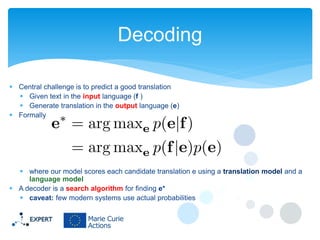
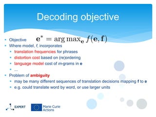
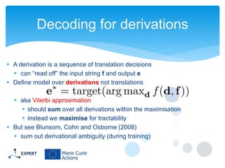
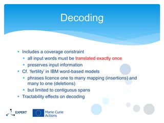
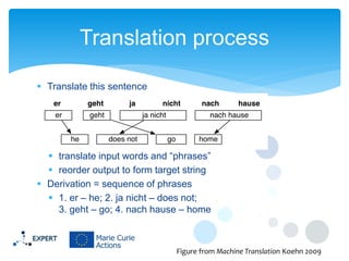
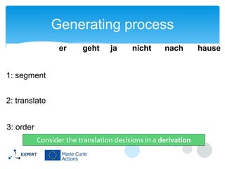
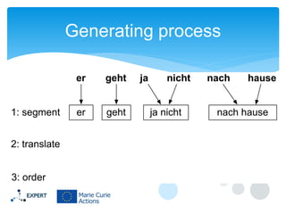
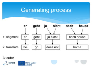
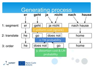
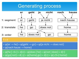
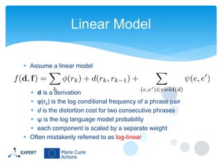
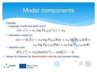
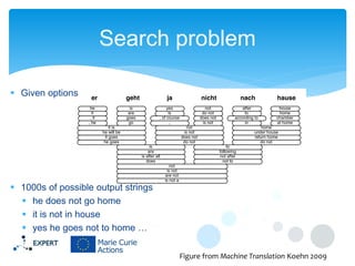
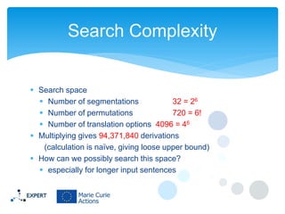
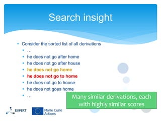
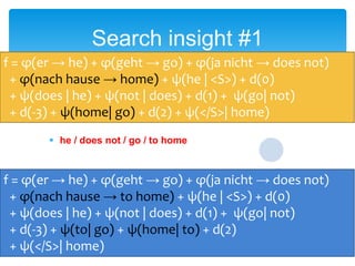
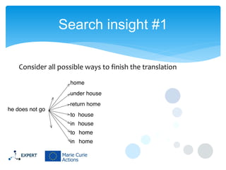
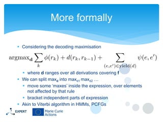
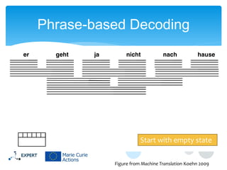
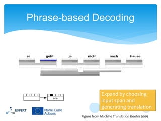
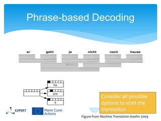
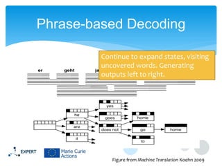
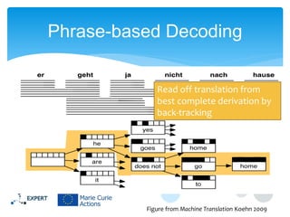
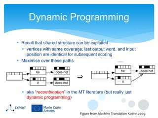
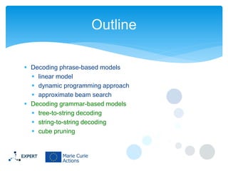
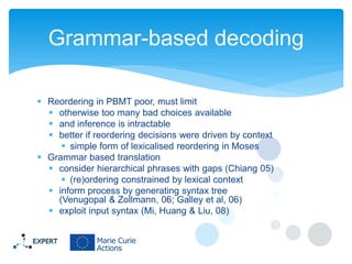
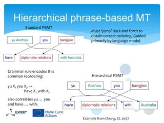
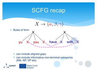
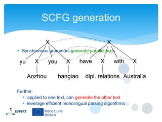
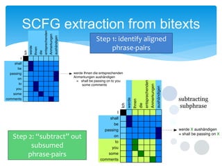
This document discusses statistical machine translation decoding. It begins with an overview of decoding objectives and challenges, such as ambiguity in possible translations. It then describes decoding phrase-based models using a linear model and dynamic programming approach, with approximations like beam search. Grammar-based decoding is also covered, including synchronous context-free grammar parsing and translation. Key challenges like search complexity and language model integration are addressed.

1. Statistical Machine Translation
Part II: Decoding
Trevor Cohn, U. Sheffield
EXPERT winter school
November 2013
Some figures taken from Koehn 2009

2. Recap
 You’ve seen several models of translation
 word-based models: IBM 1-5
 phrase-based models
 grammar-based models
 Methods for
 learning translation rules from bitexts
 learning rule weights
 learning several other features: language models,
reordering etc

3. Decoding
 Central challenge is to predict a good translation
 Given text in the input language (f )
 Generate translation in the output language (e)
 Formally
 where our model scores each candidate translation e using a translation model and a
language model
 A decoder is a search algorithm for finding e*
 caveat: few modern systems use actual probabilities

4. Outline
 Decoding phrase-based models
 linear model
 dynamic programming approach
 approximate beam search
 Decoding grammar-based models
 synchronous grammars
 string-to-string decoding

5. Decoding objective
 Objective
 Where model, f, incorporates
 translation frequencies for phrases
 distortion cost based on (re)ordering
 language model cost of m-grams in e
 ...
 Problem of ambiguity
 may be many different sequences of translation decisions mapping f to e
 e.g. could translate word by word, or use larger units

6. Decoding for derivations
 A derivation is a sequence of translation decisions
 can “read off” the input string f and output e
 Define model over derivations not translations
 aka Viterbi approximation
 should sum over all derivations within the maximisation
 instead we maximise for tractability
 But see Blunsom, Cohn and Osborne (2008)
 sum out derivational ambiguity (during training)

7. Decoding
 Includes a coverage constraint
 all input words must be translated exactly once
 preserves input information
 Cf. ‘fertility’ in IBM word-based models
 phrases licence one to many mapping (insertions) and
many to one (deletions)
 but limited to contiguous spans
 Tractability effects on decoding

8. Translation process
 Translate this sentence
 translate input words and “phrases”
 reorder output to form target string
 Derivation = sequence of phrases
 1. er – he; 2. ja nicht – does not;
3. geht – go; 4. nach hause – home
Figure from Machine Translation Koehn 2009

9. Generating process
er
geht
ja
nicht
nach
1: segment
2: translate
3: order
Consider the translation decisions in a derivation
hause

10. Generating process
er
1: segment
2: translate
3: order
geht
er
geht
ja
nicht
ja nicht
nach
hause
nach hause

11. Generating process
er
geht
1: segment
er
geht
ja nicht
nach hause
2: translate
he
go
does not
home
3: order
ja
nicht
nach
hause

12. Generating process
er
geht
1: segment
er
geht
ja nicht
1: uniform cost (ignore)
2: translate
he
3: order
he
go
ja
nicht
does not
2: TM probability
does not
go
3: distortion cost & LM
probability
nach
hause
nach hause
home
home

13. Generating process
er
geht
ja
1: segment
er
geht
ja nicht
nach hause
2: translate
he
go
does not
home
3: order
he
go
home
does not
nicht
nach
hause
f=0
+ φ(er → he) + φ(geht → go) + φ(ja nicht → does not)
+ φ(nach hause → home)
+ ψ(he | <S>) + d(0) + ψ(does | he) + ψ(not | does) + d(1)
+ ψ(go| not) + d(-3) + ψ(home| go) + d(2) + ψ(</S>| home)

14. Linear Model
 Assume a linear model
 d is a derivation
 φ(rk) is the log conditional frequency of a phrase pair
 d is the distortion cost for two consecutive phrases
 ψ is the log language model probability
 each component is scaled by a separate weight
 Often mistakenly referred to as log-linear

15. Model components
 Typically:
 language model and word count
 translation model (s)
 distortion cost
 Values of α learned by discriminative training (not covered today)

16. Search problem
 Given options
 1000s of possible output strings
 he does not go home
 it is not in house
 yes he goes not to home …
Figure from Machine Translation Koehn 2009

17. Search Complexity
 Search space
 Number of segmentations
32 = 26
 Number of permutations
720 = 6!
 Number of translation options 4096 = 46
 Multiplying gives 94,371,840 derivations
(calculation is naïve, giving loose upper bound)
 How can we possibly search this space?
 especially for longer input sentences

18. Search insight
 Consider the sorted list of all derivations
 …
 he does not go after home
 he does not go after house
 he does not go home
 he does not go to home
 he does not go to house
 he does not goes home
 …
Many similar
derivations, each
with highly similar scores

19. Search insight #1
f = φ(er → he) + φ(geht → go) + φ(ja nicht → does not)
+ φ(nach hause → home) + ψ(he | <S>) + d(0)
+ ψ(does | he) + ψ(not | does) + d(1) + ψ(go| not)
+ d(-3)  he / does not / go+/ d(2) + ψ(</S>| home)
+ ψ(home| go) home
 he / does not / go / to home
f = φ(er → he) + φ(geht → go) + φ(ja nicht → does not)
+ φ(nach hause → to home) + ψ(he | <S>) + d(0)
+ ψ(does | he) + ψ(not | does) + d(1) + ψ(go| not)
+ d(-3) + ψ(to| go) + ψ(home| to) + d(2)
+ ψ(</S>| home)

20. Search insight #1
Consider all possible ways to finish the translation

21. Search insight #1
Score ‘f’ factorises, with shared components across all options.
Can find best completion by maximising f.

22. Search insight #2
Several partial translations can be finished the same way

23. Search insight #2
Several partial translations can be finished the same way
Only need to consider maximal scoring partial translation

24. Dynamic Programming Solution
 Key ideas behind dynamic programming
 factor out repeated computation
 efficiently solve the maximisation problem
 What are the key components for “sharing”?
 don’t have to be exactly identical; need same:
 set of untranslated words
 righter-most output words
 last translated input word location
 The decoding algorithm aims to exploit this

25. More formally
 Considering the decoding maximisation
 where d ranges over all derivations covering f
 We can split maxd into maxd1 maxd2 …
 move some ‘maxes’ inside the expression, over elements
not affected by that rule
 bracket independent parts of expression
 Akin to Viterbi algorithm in HMMs, PCFGs

26. Phrase-based Decoding
Start with empty state
Figure from Machine Translation Koehn 2009

27. Phrase-based Decoding
Expand by choosing
input span and
generating translation
Figure from Machine Translation Koehn 2009

28. Phrase-based Decoding
Consider all possible
options to start the
translation
Figure from Machine Translation Koehn 2009

29. Phrase-based Decoding
Continue to expand states, visiting
uncovered words. Generating
outputs left to right.
Figure from Machine Translation Koehn 2009

30. Phrase-based Decoding
Read off translation from
best complete derivation by
back-tracking
Figure from Machine Translation Koehn 2009

31. Dynamic Programming
 Recall that shared structure can be exploited
 vertices with same coverage, last output word, and input
position are identical for subsequent scoring
 Maximise over these paths
⇒
 aka “recombination” in the MT literature (but really just
dynamic programming)
Figure from Machine Translation Koehn 2009

32. Complexity
 Even with DP search is still intractable
 word-based and phrase-based decoding is NP complete
 Knight 99; Zaslavskiy, Dymetman, and Cancedda, 2009
 whereas SCFG decoding is polynomial
 Complexity arises from
 reordering model allowing all permutations (limit)
 no more than 6 uncovered words
 many translation options (limit)
 no more than 20 translations per phrase
 coverage constraints, i.e., all words to be translated once

33. Pruning
 Limit the size of the search graph by eliminating bad paths
early
 Pharaoh / Moses
 divide partial derivations into stacks, based on number of
input words translated
 limit the number of derivations in each stack
 limit the score difference in each stack

34. Stack based pruning
Algorithm iteratively “grows” from one stack to the next
larger ones, while pruning the entries in each stack.
Figure from Machine Translation Koehn 2009

35. Future cost estimate
 Higher scores for translating easy parts first
 language model prefers common words
 Early pruning will eliminate derivations starting with the difficult words
 pruning must incorporate estimate of the cost of translating the
remaining words
 “future cost estimate” assuming unigram LM and monotone translation
 Related to A* search and admissible heuristics
 but incurs search error (see Chang & Collins, 2011)

36. Beam search complexity
 Limit the number of translation options per phrase to constant (often 20)
 # translations proportional to input sentence length
 Stack pruning
 number of entries & score ratio
 Reordering limits
 finite number of uncovered words (typically 6)
but see Lopez EACL 2009
 Resulting complexity
 O( stack size x sentence length )

37. k-best outputs
 Can recover not just the best solution
 but also 2nd, 3rd etc best derivations
 straight-forward extension of beam search
 Useful in discriminative training of feature weights, and other
applications

38. Alternatives for PBMT decoding
 FST composition (Kumar & Byrne, 2005)
 each process encoded in WFST or WFSA
 simply compose automata, minimise and solve
 A* search (Och, Ueffing & Ney, 2001)
 Sampling (Arun et al, 2009)
 Integer linear programming
 Germann et al, 2001
 Reidel & Clarke, 2009
 Lagrangian relaxation
 Chang & Collins, 2011

39. Outline
 Decoding phrase-based models
 linear model
 dynamic programming approach
 approximate beam search
 Decoding grammar-based models
 tree-to-string decoding
 string-to-string decoding
 cube pruning

40. Grammar-based decoding
 Reordering in PBMT poor, must limit
 otherwise too many bad choices available
 and inference is intractable
 better if reordering decisions were driven by context
 simple form of lexicalised reordering in Moses
 Grammar based translation
 consider hierarchical phrases with gaps (Chiang 05)
 (re)ordering constrained by lexical context
 inform process by generating syntax tree
(Venugopal & Zollmann, 06; Galley et al, 06)
 exploit input syntax (Mi, Huang & Liu, 08)

41. Hierarchical phrase-based MT
Standard PBMT
yu Aozhou
have
you
diplomatic relations
bangjiao
with Australia
Grammar rule encodes this
common reordering:
yu X1 you X2 →
have X2 with X1
also correlates yu … you
and have … with.
Must ‘jump’ back and forth to
obtain correct ordering. Guided
primarily by language model.
Hierarchical PBMT
yu
have
Aozhou
you
diplomatic relations
bangjiao
with
Example from Chiang, CL 2007
Australia

42. SCFG recap
 Rules of form
yu
X
X
you
X
X
have X
with X
 can include aligned gaps
 can include informative non-terminal categories
(NN, NP, VP etc)

43. SCFG generation
X
X
 Synchronous grammars generate parallel texts
yu
X
Aozhou
you
X
bangiao
have
X
with
X
dipl. relations Australia
Further:
 applied to one text, can generate the other text
 leverage efficient monolingual parsing algorithms

44. SCFG extraction from bitexts
Step 1: identify aligned
phrase-pairs
Step 2: “subtract” out
subsumed
phrase-pairs

45. Example grammar
X
yu
X1
you
X
X2
have X2 with X1
X
X
Aozhou
Australia
X
X
bangiao
diplomatic relations
S
S
X
X

46. Decoding as parsing
 Consider only the foreign side of grammar
Step 1: parse input text
X
yu
X
X
you
X
Aozhou bangiao
S
X
X
S
X
yu
X
Aozhou
you
X
bangiao

47. Step 2: Translate
S
S
X
X
yu
X
Aozhou
you
X
bangiao
with X
X
yu
has
you
dipl. rels
Australia
Traverse tree, replacing each input production
with its highest scoring output side
X
X
Australia
dipl. rels

48. Chart parsing
1. length = 1
X → Aozhou
X → bangjiao
S0,4
X0,4
S0,2
X2,4
X0,2
X1,2
0
4. length = 4
S→SX
X → yu X you X
X3,4
yu Aozhou you bangiao
1
2. length = 2
X → yu X
X → you X
S→X
2
3
4
Two derivations yielding S0,4
Take the one with
maximum score

49. Chart parsing for decoding
S0,4
X0,4
S0,2
X2,4
X0,2
X1,2
0
X3,4
yu Aozhou you bangiao
1
2
3
• starting at full sentence
S0,J
• traverse down to find
maximum score
derivation
• translate each rule
using the maximum
scoring right-hand side
• emit the output string
4

50. LM intersection
 Very efficient
 cost of parsing, i.e., O(n3)
 reduces to linear if we impose a maximum span limit
 translation step simple O(n) post-processing step
 But what about the language model?
 CYK assumes model scores decompose with the tree
structure
 but the language model must span constituents
Problem: LM doesn’t factorise!

51. LM intersection via lexicalised NTs
 Encode LM context in NT categories
(Bar-Hillel et al, 1964)
X → <yu X1 you X2, have X2 with X1>
haveXb
→ <yu aXb1 you cXd2, have aXb2 with cXd1>
left & right m-1 words in output translation
 When used in parent rule, LM can access boundary words
 score now factorises with tree

52. LM intersection via lexicalised NTs
X
yu
X
withXb
φTM
you
yu
X
you
φTM
Aozhou
➠
Aozhou
φTM
diplomaticXrelations
φTM
bangiao
bangiao
φTM
S
S
φTM
X
cXd
AustraliaXAustralia
X
X
aX b
φTM + ψ(with → c)
+ ψ(d → has)
+ ψ(has → a)
aXb
φTM + ψ(<S> → a)
+ ψ(b → </S>)

53. +LM Decoding
 Same algorithm as before
 Viterbi parse with input side grammar (CYK)
 for each production, find best scoring output side
 read off output string
 But input grammar has blown up
 number of non-terminals is O(T2)
 overall translation complexity of O(n3T4(m-1))
 Terrible!

54. Beam search and pruning
 Resort to beam search
 prune poor entries from chart cells during CYK parsing
 histogram, threshold as in phrase-based MT
 rarely have sufficient context for LM evaluation
 Cube pruning
 lower order LM estimate search heuristic
 follows approximate ‘best first’ order for incorporating child spans into
parent rule
 stops once beam is full
 For more details, see
 Chiang “Hierarchical phrase-based translation”. 2007. Computational
Linguistics 33(2):201–228.

55. Further work
 Synchronous grammar systems
 SAMT (Venugopal & Zollman, 2006)
 ISI’s syntax system (Marcu et al.,2006)
 HRGG (Chiang et al., 2013)
 Tree to string (Liu, Liu & Lin, 2006)
 Probabilistic grammar induction
 Blunsom & Cohn (2009)
 Decoding and pruning
 cube growing (Huang & Chiang, 2007)
 left to right decoding (Huang & Mi, 2010)

56. Summary
 What we covered
 word based translation and alignment
 linear phrase-based and grammar-based models
 phrase-based (finite state) decoding
 synchronous grammar decoding
 What we didn’t cover
 rule extraction process
 discriminative training
 tree based models
 domain adaptation
 OOV translation
 …