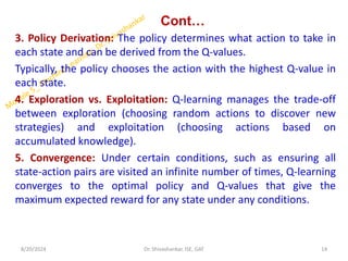
The document covers a machine learning module focused on reinforcement learning, detailing its principles, including how agents learn through feedback to maximize rewards. Key concepts such as positive and negative reinforcement, Q-learning, and the credit assignment problem are discussed, alongside algorithms used in AI applications. Additionally, the document includes examples and mathematical formulations for Q-value updates and explores the interplay between exploration and exploitation in reinforcement learning.

1. MACHINE LEARNING (INTEGRATED)
(21ISE62)
Module 5
Dr. Shivashankar
Professor
Department of Information Science & Engineering
GLOBAL ACADEMY OF TECHNOLOGY-Bengaluru
8/20/2024 1
Dr. Shivashankar, ISE, GAT
GLOBAL ACADEMY OF TECHNOLOGY
Ideal Homes Township, Rajarajeshwari Nagar, Bengaluru – 560 098
Department of Information Science & Engineering

2. Course Outcomes
After Completion of the course, student will be able to:
 Illustrate Regression Techniques and Decision Tree Learning
Algorithm.
 Apply SVM, ANN and KNN algorithm to solve appropriate problems.
 Apply Bayesian Techniques and derive effective learning rules.
 Illustrate performance of AI and ML algorithms using evaluation
techniques.
 Understand reinforcement learning and its application in real world
problems.
Text Book:
1. Tom M. Mitchell, Machine Learning, McGraw Hill Education, India Edition 2013.
2. EthemAlpaydın, Introduction to machine learning, MIT press, Second edition.
3. Pang-Ning Tan, Michael Steinbach, Vipin Kumar, Introduction to Data Mining,
Pearson, First Impression, 2014.
8/20/2024 2
Dr. Shivashankar, ISE, GAT

3. Module 5: Reinforcement Learning
• Reinforcement learning (RL) is a Machine Learning (ML) technique that
trains software to make decisions to achieve the most optimal results.
• It mimics the trial-and-error learning process that humans use to
achieve their goals.
• It is a feedback based ML approach, here an agent learns to which
action to perform by looking at the environment and result of action.
• For each correct action, the agents get positive feedback, and for each
incorrect action, the agent gets negative feedback or penalty.
8/20/2024 3
Dr. Shivashankar, ISE, GAT
Agent
Environment
Action
State
Rewards
Fig 5.1: Reinforcement Learning

4. Learning to Optimize Rewards
• The agent interact with environment and identify the possible action he can
perform.
• The primary goal of an agent in reinforcement learning is to perform actions by
looking at the environment and get the maximum positive rewards.
• In reinforcement learning, the agent learns automatically using feedbacks
without any labelled data, unlike supervised learning.
• Since there is no labelled data, so the agent is bound to learn by its experience
only.
• There are two types of reinforcement learning: Positive and negative.
• Positive reinforcement learning is a recurrence behavior due to positive
rewards.
• Rewards increase strength and frequency of a specific behavior.
• This encourages to execute similar action that yield maximum rewards.
• Similarly in negative reinforcement learning, negative rewards are used as
deterrent to weaken the behavior and to avoid it.
• Rewards decrease the strength and the frequency of a specific behavior.
8/20/2024 4
Dr. Shivashankar, ISE, GAT

5. Cont…
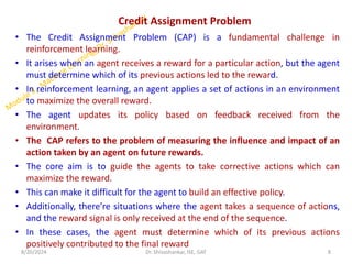
• The agent can take any path to reach to the final point, but he needs to make
it in possible fewer steps. Suppose the agent considers the path S9-S5-S1-S2-
S3, so he will get the +1-reward point.
• Action performed by the agent is referred to as "a"
• State occurred by performing the action is "s."
• The reward/feedback obtained for each good and bad action is "R."
• A discount factor is Gamma "γ."
V(s) = max [R(s,a) + γV(s`)]
8/20/2024 5
Dr. Shivashankar, ISE, GAT

6. Cont…
• V(s)= value calculated at a particular point.
• R(s,a) = Reward at a particular state s by performing an action.
• γ = Discount factor
• V(s`) = The value at the previous state.
How to represent the agent state?
• We can represent the agent state using the Markov State that contains all
the required information from the history. The State St is Markov state if it
follows the given condition:
P[St+1 | St ] = P[St +1 | S1,......, St]
• tuple of four elements (S, A, Pa, Ra):
• A set of finite States S
• A set of finite Actions A
• Rewards received after transitioning from state S to state S', due to action
a.
• Probability Pa.
8/20/2024 6
Dr. Shivashankar, ISE, GAT

7. Reinforcement Learning Algorithms
• Reinforcement learning algorithms are mainly used in AI applications and gaming
applications. The main used algorithms are:
• Q-Learning:
• Q-learning is an Off policy RL algorithm, which is used for the temporal difference
Learning. The temporal difference learning methods are the way of comparing
temporally successive predictions.
• It learns the value function Q (S, a), which means how good to take action "a" at a
particular state "s."
• The below flowchart explains the working of Q- learning:
8/20/2024 7
Dr. Shivashankar, ISE, GAT

8. Credit Assignment Problem
• The Credit Assignment Problem (CAP) is a fundamental challenge in
reinforcement learning.
• It arises when an agent receives a reward for a particular action, but the agent
must determine which of its previous actions led to the reward.
• In reinforcement learning, an agent applies a set of actions in an environment
to maximize the overall reward.
• The agent updates its policy based on feedback received from the
environment.
• The CAP refers to the problem of measuring the influence and impact of an
action taken by an agent on future rewards.
• The core aim is to guide the agents to take corrective actions which can
maximize the reward.
• This can make it difficult for the agent to build an effective policy.
• Additionally, there’re situations where the agent takes a sequence of actions,
and the reward signal is only received at the end of the sequence.
• In these cases, the agent must determine which of its previous actions
positively contributed to the final reward
8/20/2024 8
Dr. Shivashankar, ISE, GAT

9. Cont…
• Example: As the agent explores the maze, it receives a reward of +10 for
reaching the goal state. Additionally, if it hits a stone, we penalize the action by
providing a -10 reward.
Path 1: 1-5-9
Path 2: 1-4-8
Path 3: 1-2-3-6-9
Path 4: 1-2-5-9
and so on..
8/20/2024 9
Dr. Shivashankar, ISE, GAT

10. Temporal Difference Learning
• Temporal Difference Learning in reinforcement learning works as
an unsupervised learning method.
• It helps predict the total expected future reward.
• At its core, Temporal Difference Learning (TD Learning) aims to
predict a variable's future value in a state sequence. TD Learning
made a big leap in solving reward prediction problems.
8/20/2024 10
Dr. Shivashankar, ISE, GAT
Figure 3 : The temporal difference reinforcement learning algorithm.

11. Cont…
• More formally, according to the TD algorithm the prediction error δ(t) is
defined as the immediate reward R(t) plus the predicted future value V(t+1)
minus the current value prediction V(t) (Eqn (1)):
δ (t) = R(t) + γ · V (t+1) − V (t) -----(1)
• The Pe δ(t) is used to update the old value prediction (Eqn (2)):
V (t) new = Vt(old) + α · δ (t) ----(2)
• Alpha (α): learning rate
It shows how much our estimates should be adjusted, based on the error. This
rate varies between 0 and 1.
• Gamma (γ): the discount rate
This indicates how much future rewards are valued.
• The (exponential) discount factor 0<γ<1 in Eqn (1) accounts for the fact that
humans (and other animals) tend to discount the value of future reward.
• The learning rate 0<α<1 in Eqn (2) determines how much a specific event
affects future value predictions. A learning rate close to 1 would suggest that
the most recent outcome has a strong effect on the value prediction.
8/20/2024 11
Dr. Shivashankar, ISE, GAT

12. Q-learning
• Q-learning is a reinforcement learning algorithm that finds an
optimal action-selection policy for any finite Markov Decision
Process (MDP).
• It helps an agent learn to maximize the total reward over time
through repeated interactions with the environment, even when
the model of that environment is not known.
How Does Q-Learning Work
1. Learning and Updating Q-values:
• The algorithm maintains a table of Q-values for each state-action
pair.
• These Q-values represent the expected utility of taking a given
action in a given state and following the optimal policy after that.
• The Q-values are initialized arbitrarily and are updated iteratively
using the experiences gathered by the agent.
8/20/2024 12
Dr. Shivashankar, ISE, GAT

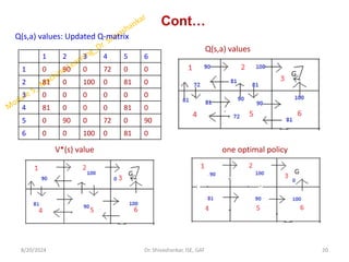
13. Q-learning
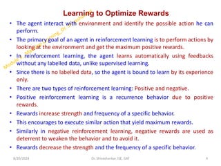
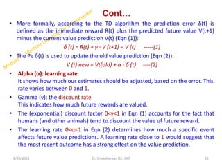
2. Q-value Update Rule:
The Q-values are updated using the formula:
𝑄(𝑠,𝑎)←𝑄(𝑠,𝑎)+𝛼[𝑟+𝛾max (𝑄(𝑠′,𝑎′)−𝑄(𝑠,𝑎))]
Q(s,a) = r(s,a) + 𝛼*max (𝑄(𝛿(s,a), ƴ
𝑎))
Where :
𝑠 is the current state,
𝑎 is the action taken,
r is the reward received after taking action 𝑎 in state 𝑠,
𝑠′ is the new state after action,
𝑎′ is any possible action from the new state 𝑠′,
𝛼 is the learning rate (0 < α ≤ 1),
𝛾 is the discount factor (0 ≤ γ < 1).
8/20/2024 13
Dr. Shivashankar, ISE, GAT

14. Cont…
3. Policy Derivation: The policy determines what action to take in
each state and can be derived from the Q-values.
Typically, the policy chooses the action with the highest Q-value in
each state.
4. Exploration vs. Exploitation: Q-learning manages the trade-off
between exploration (choosing random actions to discover new
strategies) and exploitation (choosing actions based on
accumulated knowledge).
5. Convergence: Under certain conditions, such as ensuring all
state-action pairs are visited an infinite number of times, Q-learning
converges to the optimal policy and Q-values that give the
maximum expected reward for any state under any conditions.
8/20/2024 14
Dr. Shivashankar, ISE, GAT

15. Q Learning Algorithm
For each s, a initialize the table entry ෡
𝑸(s,a) to zero.
Observe current state s.
Do forever:
 Select an action a and execute it.
 Receive immediate reward r
 Observe new state ƴ
𝒔
 Update the entry for ෡
𝑸(s,a) as follow:
Q(s,a) = r(s,a) + 𝛼*max (𝑄(𝛿(s,a), ƴ
𝑎))
෡
𝑸(s,a) ← 𝒓 + 𝜸 𝒎𝒂𝒙
ƴ
𝒂
෡
𝑸 ( ƴ
𝒔, ƴ
𝒂)
S ← ƴ
𝒔
8/20/2024 15
Dr. Shivashankar, ISE, GAT

16. Problem
Problem 1: Suppose there are 6 rooms in the given table, room 3 is the goal, have an
instant reward of 100, other rooms not directly connected to the target room have zero
reward. Each row contains an instant reward value. Construct a reward matrix, Q-learning
and calculate immediate reward value for each instant. Learning rate is 0.9.
Solution: Reward Matrix Q-learning Matrix
8/20/2024 16
Dr. Shivashankar, ISE, GAT
1 2 3 4 5 6
1 -1 0 -1 0 -1 -1
2 0 -1 100 -1 0 -1
3 -1 -1 0 -1 -1 -1
4 0 -1 -1 -1 0 -1
5 -1 0 -1 0 -1 0
6 -1 -1 100 -1 0 -1
1 2 3 4 5 6
1 0 0 0 0 0 0
2 0 0 0 0 0 0
3 0 0 0 0 0 0
4 0 0 0 0 0 0
5 0 0 0 0 0 0
6 0 0 0 0 0 0
R=
State
Action
Q=

17. Cont…
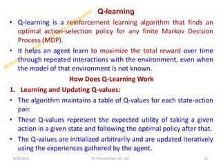
Q(state, action)= R(state, action) + Alpha * Max[Q(next state, all action)]
Q(s,a) = r(s,a) + 𝛼*max [𝑄(𝛿(s,a), ƴ
𝑎)]
At state 3: Q(2,3) = R(2,3) + 0.9 * max [Q(3,3)]
= 100 + 0.9 * max [0]
= 100 + 0 = 100
Q(6,3) = R(6,3) + 0.9 * max [Q(3,3)]
= 100 + 0.9 * max [0]
= 100 + 0 = 100
At state 2: Q(1,2) = R(1,2) + 0.9 * max [Q(2,3), Q(2,5)]
= 0 + 0.9 * max [100,0]
= 0.9*100 = 90
At state 1: Q(2,1) = R(2,1) + 0.9 * max [Q(1,2), Q(1,4)]
= 0 + 0.9 * max [90,0]
= 0.9*90 = 81
Q(4,1) = R(4,1) + 0.9 * max [Q(1,2), Q(1,4)]
= 0 + 0.9 * max [90,0]
= 0.9*90=81
8/20/2024 17
Dr. Shivashankar, ISE, GAT
Sate transition diagram

18. Cont…
At state 4: Q(1,4) = R(1,4) + 0.9 * max [Q(4,1), Q(4,5)]
= 0 + 0.9 * max [81,0]
= 0.9*81 = 72
At state 2: Q(5,2) = R(5,2) + 0.9 * max [Q(2,1), Q(2,3), Q(2,5)]
= 0 + 0.9 * max [81,100,0]
= 0.9*100 = 90
At state 4: Q(5,4) = R(5,4) + 0.9 * max [Q(4,1), Q(4,5)]
= 0 + 0.9 * max [81,0]
= 0.9*81 = 72
At state 5: Q(2,5) = R(2,5) + 0.9 * max [Q(5,2), Q(5,4), Q(5,6)]
= 0 + 0.9 * max [90, 72, 0]
= 0.9*90 = 81
Q(4,5) = R(4,5) + 0.9 * max [Q(5,2), Q(5,4), Q(5,6)]
= 0 + 0.9 * max [90, 72, 0]
= 0.9*90 = 81
8/20/2024 18
Dr. Shivashankar, ISE, GAT

19. Cont…
At state 5: Q(6,5) = R(6,5) + 0.9 * max [Q(5,2), Q(5,4), Q(5,6)]
= 0 + 0.9 * max [90, 72, 0]
= 0.9*90 = 81
At state 6: Q(5,6) = R(5,6) + 0.9 * max [Q(6,3), Q(6,5)]
= 0 + 0.9 * max [100,81]
= 0.9*100 = 90
8/20/2024 19
Dr. Shivashankar, ISE, GAT

20. Cont…
Q(s,a) values: Updated Q-matrix
Q(s,a) values
V*(s) value one optimal policy
8/20/2024 20
Dr. Shivashankar, ISE, GAT
1 2 3 4 5 6
1 0 90 0 72 0 0
2 81 0 100 0 81 0
3 0 0 0 0 0 0
4 81 0 0 0 81 0
5 0 90 0 72 0 90
6 0 0 100 0 81 0

21. Cont…
Problem 2: Suppose we have 5 rooms in a building connected by doors as shown in figure
below. We’ll number each room 0 through 4. The outside of the building can be thought of
us one big room (5). Note that doors 1 and 4 lead into the building from room 5 (outside).
The goal room is number 5. The doors that lead immediately to the goal have an instant
reward of 100. other rooms not directly connected the target room have 0 reward.
Construct a reward matrix, Q-learning and calculate immediate reward value for each
instant. Learning rate is 0.8.
8/20/2024 21
Dr. Shivashankar, ISE, GAT

22. Cont…
Solution:
Reward Matrix Q-Learning Matrix
R= Q=
8/20/2024 22
Dr. Shivashankar, ISE, GAT
0 1 2 3 4 5
0 -1 -1 -1 -1 0 -1
1 -1 -1 -1 0 -1 100
2 -1 -1 -1 0 -1 -1
3 -1 0 0 -1 0 -1
4 0 -1 -1 0 -1 100
5 -1 0 -1 -1 0 100
Action
State
0 1 2 3 4 5
0 0 0 0 0 0 0
1 0 0 0 0 0 0
2 0 0 0 0 0 0
3 0 0 0 0 0 0
4 0 0 0 0 0 0
5 0 0 0 0 0 0

23. Cont…
• Now let’s imagine what would happen if our agent were in state 5 (next state)
• Look at the 6th row of the reward matrix R(i.e. state 5)
• It has 3 possible actions: go to state 1,4, or 5.
Q(s,a) = r(s,a) + 𝛼*max [𝑄(𝛿(s,a), ƴ
𝑎)]
Q(state, action)= R(state, action) + Alpha * max[Q(next state, all action)]
At state 5:
Q(1,5) = R(1,5) + 0.8 * max [Q(5,1), Q(5,4)]
= 100 + 0.8 * max [Q(0,0)]
= 100 + 0.8*0 = 100
Q(4,5) = R(4,5) + 0.8 * max [Q(5,1), Q(5,4)]
= 100 + 0.8 * max [0,0]= 100
At state 1:
Now we imagine that we are in state 1(next state).
It has 2 possible actions: go to state 3 or state 5.
Then, we complete the Q value:
Q(3,1) = R(3,1) +0.8*Max(Q[1,3), Q(1,5)]
= 0 + 0.8 * max [0,100]
= 0 + 0.8*max(0,100) = 80
8/20/2024 23
Dr. Shivashankar, ISE, GAT

24. Cont…
Q(5,1) = R(5,1) + 0.8*max (Q(1,3), Q(1,5)]
= 0 + 0.8* max(64,100)]
0.8*100 = 80
At state 3:
Q(1,3) = R(1,3) + 0.8 * max [Q(3,1), Q(3,2), Q(3,4)]
= 0 + 0.8 * max [80, 0, 0]
= 0+ 0.8*80 = 64
Q(4,3) = R(4,3) + 0.8 * max [Q(3,4), Q(3,2), Q(3,1)]
= 0 + 0.8 * max [0, 0, 80]
= 0+ 0.8*80 = 64
Q(2,3) = R(2,3) + 0.8 * max [Q(3,2), Q(3,1), Q(3,4)]
= 0 + 0.8 * max [0, 80, 0]
= 0+ 0.8*80 = 64
At state 4:
Q(5, 4) = R(5, 4) + 0.8 * max [Q(4,5), Q(4,3), Q(4, 0)]
= 0 + 0.8 * max [100, 64, 0]
= 80
8/20/2024 24
Dr. Shivashankar, ISE, GAT

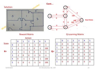
25. Cont…
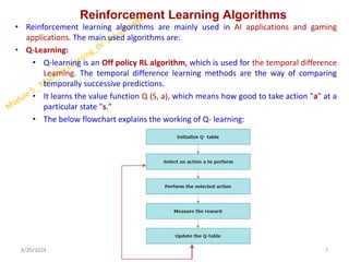
Q(3, 4) = R(3, 4) + 0.8 * max [Q(4,3), Q(4,5), Q(4, 0)]
= 0 + 0.8 * max [64,100, 0]= 80
Q(0, 4) = R(0, 4) + 0.8 * max [Q(4,0), Q(4,3), Q(4,5)]
= 0 + 0.8 * max [0, 0, 100] = 80
At state 2:
Q(3,2) = R(3,2) + 0.8*max[ Q(2,3)]
= 0 + 0.8*max[64] = 51
At state 0:
Q(4, 0) = R(4,0) + 0.8*max[Q(0,4)]
= 0 + 0.8 * 80 = 64
8/20/2024 25
Dr. Shivashankar, ISE, GAT
0 1 2 3 4 5
0 0 0 0 0 80 0
1 0 0 0 64 0 100
2 0 0 0 64 0 0
3 0 80 51 0 80 0
4 64 0 0 64 0 100
5 0 80 0 0 80 100
Updated state diagram
Final Updated Q-Learning Matrix

26. Cont…
Case Study:
Artificial Intelligence Powering Google Products,
Recent AI Tools leveraged by Tesla, AI for
Facebook,
Robo-Banking: Artificial Intelligence at JPMorgan
Chase, Audio AI,
A Machine Learning Approach — Building a Hotel
Recommendation Engine
8/20/2024 26
Dr. Shivashankar, ISE, GAT