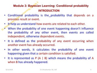
Module 3_Machine Learning Bayesian Learn

MACHINE LEARNING (INTEGRATED)
(21ISE62)
Module 3
Dr. Shivashankar
Professor
Department of Information Science & Engineering
GLOBAL ACADEMY OF TECHNOLOGY-Bengaluru
8/13/2024 1
Dr. Shivashankar, ISE, GAT
GLOBAL ACADEMY OF TECHNOLOGY
Ideal Homes Township, Rajarajeshwari Nagar, Bengaluru – 560 098
Department of Information Science & Engineering

Course Outcomes
After Completion of the course, student will be able to:
 Illustrate Regression Techniques and Decision Tree Learning
Algorithm.
 Apply SVM, ANN and KNN algorithm to solve appropriate problems.
 Apply Bayesian Techniques and derive effective learning rules.
 Illustrate performance of AI and ML algorithms using evaluation
techniques.
 Understand reinforcement learning and its application in real world
problems.
Text Book:
1. Tom M. Mitchell, Machine Learning, McGraw Hill Education, India Edition 2013.
2. EthemAlpaydın, Introduction to machine learning, MIT press, Second edition.
3. Pang-Ning Tan, Michael Steinbach, Vipin Kumar, Introduction to Data Mining,
Pearson, First Impression, 2014.
8/13/2024 2

Module 3: Bayesian Learning: Conditional probability
INTRODUCTION
• Conditional probability is the probability that depends on a
previous result or event.
• It help us understand how events are related to each other.
• When the probability of one event happening doesn’t influence
the probability of any other event, then events are called
independent, otherwise dependent events.
• It is defined as the probability of any event occurring when
another event has already occurred.
• In other words, it calculates the probability of one event
happening given that a certain condition is satisfied.
• It is represented as P (A | B) which means the probability of A
when B has already happened.
8/13/2024 3

Cont…
Conditional Probability Formula:
• When the intersection of two events happen, then the formula for conditional
probability for the occurrence of two events is given by;
• P(A|B) = N(A∩B)/N(B) or
• P(B|A) = N(A∩B)/N(A)
• Where P(A|B) represents the probability of occurrence of A given B has occurred.
• N(A ∩ B) is the number of elements common to both A and B.
• N(B) is the number of elements in B, and it cannot be equal to zero.
• Let N represent the total number of elements in the sample space.
• N(A ∩ B)/N can be written as P(A ∩ B) and N(B)/N as P(B).
𝑃 𝐴 𝐵 =
𝑃 𝐵 𝐴 𝑃(𝐴)
𝑃(𝐵)
• Therefore, P(A ∩ B) = P(B) P(A|B) if P(B) ≠ 0
• = P(A) P(B|A) if P(A) ≠ 0
• Similarly, the probability of occurrence of B when A has already occurred is given by,
• P(B|A) = P(B ∩ A)/P(A)
8/13/2024 4

Cont…
How to Calculate Conditional Probability?
To calculate the conditional probability, we can use the following method:
Step 1: Identify the Events. Let’s call them Event A and Event B.
Step 2: Determine the Probability of Event A i.e., P(A)
Step 3: Determine the Probability of Event B i.e., P(B)
Step 4: Determine the Probability of Event A and B i.e., P(A∩B).
Step 5: Apply the Conditional Probability Formula and calculate the required
probability.
Conditional Probability of Independent Events
For independent events, A and B, the conditional probability of A and B with respect to
each other is given as follows:
P(B|A) = P(B)
P(A|B) = P(A)
8/13/2024 5

Cont…
Problem 1: Two dies are thrown simultaneously, and the sum of the numbers obtained is
found to be 7. What is the probability that the number 3 has appeared at least once?
Solution:
• Event A indicates the combination in which 3 has appeared at least once.
• Event B indicates the combination of the numbers which sum up to 7.
• A = {(3, 1), (3, 2), (3, 3)(3, 4)(3, 5)(3, 6)(1, 3)(2, 3)(4, 3)(5, 3)(6, 3)}
• B = {(1, 6)(2, 5)(3, 4)(4, 3)(5, 2)(6, 1)}
• P(A) = 11/36
• P(B) = 6/36
• A ∩ B = 2
• P(A ∩ B) = 2/36
• Applying the conditional probability formula we get,
• P(A|B) = P(A∩B)/P(B) = (2/36)/(6/36) = ⅓
8/13/2024 6

Cont…
Problem 2: In a group of 100 computer buyers, 40 bought CPU, 30 purchased monitor,
and 20 purchased CPU and monitors. If a computer buyer chose at random and bought a
CPU, what is the probability they also bought a Monitor?
Solution:
As per the first event, 40 out of 100 bought CPU,
So, P(A) = 40% or 0.4
Now, according to the question, 20 buyers purchased both CPU and monitors. So, this is
the intersection of the happening of two events. Hence,
P(A∩B) = 20% or 0.2
Conditional probability is
P(B|A) = P(A∩B)/P(B)
P(B|A) = 0.2/0.4 = 2/4 = ½ = 0.5
The probability that a buyer bought a monitor, given that they purchased a CPU, is 50%.
8/13/2024 7

Cont…
Question 7: In a survey among a group of students, 70% play football, 60% play
basketball, and 40% play both sports. If a student is chosen at random and it is
known that the student plays basketball, what is the probability that the
student also plays football?
Solution:
Let’s assume there are 100 students in the survey.
Number of students who play football = n(A) = 70
Number of students who play basketball = n(B) = 60
Number of students who play both sports = n(A ∩ B) = 40
To find the probability that a student plays football given that they play
basketball, we use the conditional probability formula:
P(A|B) = n(A ∩ B) / n(B)
Substituting the values, we get:
P(A|B) = 40 / 60 = 2/3
Therefore, probability that a randomly chosen student who plays basketball also
plays football is 2/3.
8/13/2024 8

BAYES THEOREM
• Bayes’ theorem describes the probability of occurrence of an event related to any
condition.
• Bayes’ Theorem is used to determine the conditional probability of an event.
• Bayesian methods provide the basis for probabilistic learning methods that
accommodate knowledge about the prior probabilities of alternative hypotheses.
• To define Bayes theorem precisely:
• P(h) to denote the initial probability that hypothesis h holds.
• P(h) is often called the prior-probability of h and may reflect any background
knowledge, chance that h is a correct hypothesis.
• P(D) to denote the prior probability that training data D will be observed (i.e., the
probability of D given no knowledge about which hypothesis holds).
• P(D|h) to denote the probability of observing data D given some world in which
hypothesis h holds.
• P (h|D) is called the posterior-probability of h, because it reflects our confidence that h
holds.
• Notice the posterior probability P(h|D) reflects the influence of the training data D, in
contrast to the prior probability P(h) , which is independent of D.
8/13/2024 9

BAYES THEOREM
• If A and B are two events, then the formula for the Bayes theorem is given by:
• P(A|B) =
P(B|A) X P(A)
𝑃(𝐵)
• Where P(A|B) is the probability of condition when event A is occurring while event B has
already occurred.
P(A) – Probability of event A
P(B) – Probability of event B
P(A|B) – Probability of A given B
P(B|A) – Probability of B given A
From the definition of conditional probability, Bayes theorem can be derived for events as given
below:
P(A|B) = P(A ⋂ B)/ P(B), where P(B) ≠ 0
P(B|A) = P(B ⋂ A)/ P(A), where P(A) ≠ 0
• Since P(A∩ 𝐵)𝑎𝑛𝑑 𝑃(𝐵 ∩ 𝐴) are equal
• P(A|B) X P(B) = P(B|A) X P(A)
∴ P(A|B) =
P(B|A) X P(A)
𝑃(𝐵)
this is the Bays theorem.
8/13/2024 10
Likelihood
probability
Posterior
probability
Marginal
probability
Prior probability

Cont…
Problem 1: A patient takes a lab test for cancer diagnosis. There are two possible
outcomes in this case: ⊕(positive) and ⊖ (negative). The test returns a correct positive
results in only 98%. If the cases in which the diseases is actually present and a correct
negative result in only 97% of the cases in which the disease in present. Furthermore,
0.008 of the entire population have this cancer.
Compute the following values.
1). P(Cancer) 2). P(¬𝐶𝑎𝑛𝑐𝑒𝑟) 3). P(+ve Cancer)
4). P(-ve Cancer) 5). P(+| (¬𝐶𝑎𝑛𝑐𝑒𝑟) 4). P(-| (¬𝐶𝑎𝑛𝑐𝑒𝑟)
Solution:
• P(cancer)= 0.008 P(¬cancer)= 0.992
• P(⊕/cancer)=0.98 P(⊖/cancer)= 0.02
• P(⊕/¬cancer)=0.03 P(⊖/¬cancer)= 0.97 and
• P(⊕/cancer) P(cancer)=0.98 X 0.008 = 0.0078
• P(⊕/-cancer) P(-cancer)=0.03 X 0.992=0.0298
• Thus, ℎ𝑀𝐴𝑃 = -cancer.
• The exact posterior probabilities can also be determined by normalizing the above
quantities so that they sum to 1 (e.g., P(cancer/ ⊕) =
0.0078
0.0078+0.0298
= 0.207
8/13/2024 11

Cont…
Problem 3: Given that they passed the exam what is the probability it is a woman ?
Answer:
P(A): Probability of a woman passing the exam is 92/100 and it's equal to 0.92
P(B|A): probability of having a woman ; 100/200 and it's equal to 0.5
P(B): The probability of passing the exam ; 169/200 and it's equal to 0.845
P(A|B) = (P(0.5) x P(0.92 ) / P(0.845)
P(A|B) = 0.54
92/169 = 0.54 too
8/13/2024 12
Did not pass
the exam
Passed the
exam
Total
Women 8 92 100
Men 23 77 100
Total 31 169 200

Cont…
4. Covid-19 has taken over the world and the use of Covid19 tests is still relevant to block
the spread of the virus and protect our families.
If the Covid19 infection rate is 10% of the population, and thanks to the tests we have in
Algeria, 95% of infected people are positive with 5% false positive.
What would be the probability that I am really infected if I test positive?
Solution :
Parameters :
• P(A): 10% infected
• P(B|A): 95% Test positive while infected
• 5% False positive while non infected
• 90% not infected
• We will start multiplying the probability of infection (10%) by the probability of testing
positive given that be infected (95%) then we divided by the sum of the probability of
infection (10%) by the probability of testing positive given that be infected (95%) with
not infected (90%) multiplied by false positive (5%)
P(A|B) = P(A) * P(B|A) / Σ P(A) * P(B|A)
P(A|B) = 0.1 * 0.95 /(0.95 * 0.1) +(0.05*0.90)
P(A|B) = 0.095 / 0.095 + 0.045
P(A|B) = 0.678
8/13/2024 13

Cont…
2. Let A denote the event that a “patient has liver disease”, and B the event that a “patient
is an alcoholic”. It is known from experience that 10% of the patients entering the clinic
have liver disease and 5% of the patient are alcoholics.
Also, among those patients diagnosed with liver disease, 7% are alcoholic. Given that a
patient is alcoholic, what is the probability that he will have liver disease?
Solution:
A-”patient has liver disease”.
B-”patient is an alcoholic”.
P(A)=10%=0.1
P(B)=5%=0.05
P(B|A)=7%=0.07
P(A|B) =
P(B|A) X P(A)
𝑃(𝐵)
=
0.07𝑋0.10
0.05
= 0.14
8/13/2024 14

MAXIMUM LIKELIHOOD AND LEAST-SQUARED ERROR
HYPOTHESES
• Many learning approaches such as neural network learning, linear regression, and
polynomial curve fitting try to learn a continuous valued target function.
• Under certain assumptions any learning algorithm that minimizes the squared error
between output hypothesis predictions and the training data will output a MAXIMUM
LIKELIHOOD HYPOTHESIS.
• The significance of this result is that it provides a Bayesian justification (under certain
assumptions) for many neural network and other curve fitting methods that attempt to
minimize the sum of squared errors over the training data.
• In order to find the Maximum Likelihood Hypothesis in Bayesian learning for
continuous valued target function, we start with Maximum Likelihood Hypothesis
definition, but using lower case p to refer to the Probability Density Function
ℎ𝑀𝐿 = argmax
ℎ𝜖𝐻
𝑝 𝐷|ℎ
8/13/2024 15
The argument that gives the maximum
value from a target function

HYPOTHESES
• ℎ𝑀𝐿 = argmax
ℎ𝜖𝐻
𝑝 𝐷|ℎ where p: probability density function
• Assume that fixed set of training instances ( 𝑥1, 𝑥2 , 𝑥3 ,……. 𝑥𝑛 ) and data D
corresponding sequence of target values D=(𝑑1, 𝑑2, … . 𝑑𝑛)
• p(D|h) → product of p(𝑑𝑖|ℎ)
ℎ𝜖𝐻
ෑ
𝑖=1
𝑛
𝑝(𝑑𝑖|ℎ)
Assume target values are normally distributed
𝑓(𝑥|𝜇)=
1
2𝜋𝜎2
𝑒
−
𝑥−𝜇 2
2𝜎2
ℎ𝜖𝐻
ෑ
𝑖=1
𝑛
𝑝(𝑑𝑖|ℎ)
ℎ𝜖𝐻
ෑ
𝑖=1
𝑛
1
2𝜋𝜎2
𝑒
−
1
2𝜎2 𝑑𝑖−𝜇 2
ℎ𝜖𝐻
ෑ
𝑖=1
𝑛
1
2𝜋𝜎2
𝑒
−
1
2𝜎2 𝑑𝑖−ℎ(𝑥𝑖) 2
8/13/2024 16
Mean
Standard
Deviation
Target of
𝑖𝑡ℎ
input
output of hypothesis
𝑜𝑓 𝑖𝑡ℎ
input
Variance

Conti..
Rather than maximizing above calculated expression, we shall choose to maximize its (less
complicated) logarithmic.
This is justified because Ln(p) is a monotonic function of p. Therefore maximizing Ln p also
maximizes p.
ℎ𝜖𝐻
෍
𝑖=1
𝑚
𝑙𝑛
1
2𝜋𝜎2
−
1
2𝜎2 𝑑𝑖 − ℎ(𝑥𝑖 )2
First term is constant, discard it
ℎ𝜖𝐻
෍
𝑖=1
𝑚
−
1
2𝜎2 𝑑𝑖 − ℎ(𝑥𝑖 )2
Maximizing the negative quantity is equivalent to minimizing the corresponding position
quantity.
ℎ𝜖𝐻
෍
𝑖=1
𝑚
1
2𝜎2
𝑑𝑖 − ℎ(𝑥𝑖 )2
Finally we can again discard constants that are independent of h
ℎ𝜖𝐻
෍
𝑖=1
𝑚
8/13/2024 17
Leas square error hypothesis Bayesian
Learning for given continuous valued target

NAIVE BAYES CLASSIFIER
• Naïve Bayes algorithm is a supervised learning algorithm, which is based
on Bayes theorem (helps to determine the likelihood that one event will occur
with unclear information while another has already happened) and used for
solving classification problems.
• It is mainly used in text classification that includes a high-dimensional training
dataset.
• Naïve Bayes Classifier is one of the simple and most effective Classification
algorithms which helps in building the fast machine learning models that can
make quick predictions.
• It is a probabilistic classifier, which means it predicts on the basis of the
probability of an object.
• Naïve: It assumes that the occurrence of a certain feature is independent of
the occurrence of other features.
• Example: If the fruit is identified on the bases of color, shape, and taste, then
red, spherical, and sweet fruit is recognized as an apple. Hence each feature
individually contributes to identify that it is an apple without depending on
each other.
8/13/2024 18

Conti..
Naïve and Bayes algorithm : It is a way to calculate the value of P(B|A) with the
knowledge of P(A|B).
Working of Naïve Bayes' Classifier:
 Convert the given dataset into frequency tables (divide the number of rows
and columns).
 Generate Likelihood table by finding the probabilities of given features
(𝜇, 𝜎, 𝑥𝑖).
 Now, use Bayes theorem to calculate the posterior probability.
Steps to implement:
• Step 1: Data Pre-processing step
• Step 2: Fitting Naive Bayes to the Training set
• Step 3: Predicting the test result
• Step 4: Test accuracy of the result
• Step 5: Visualizing the test set result.
8/13/2024 19

• One highly practical Bayesian learning method is the naive Bayes learner, often called
the Naive Bayes classifier.
• The naive Bayes classifier applies to learning tasks where each instance x is described
by a conjunction of attribute values and where the target function f (x) can take on any
value from some finite set V.
• A set of training examples of the target function is provided, and a new instance is
presented, described by the tuple of attribute values 𝑎1, 𝑎2, 𝑎3, … , 𝑎𝑛 .
• The learner is asked to predict the target value, or classification, for this new instance.
• The naive Bayes classifier is based on the simplifying assumption that the attribute
values are conditionally independent given the target value.
• Naive Bayes classifier:
𝑉𝑁𝐵 = 𝑎𝑟𝑔𝑚𝑎𝑥
𝑣𝑗𝜖𝑣
𝑣𝑖 ෑ
𝑖
𝑃(𝑎𝑖|𝑣𝑗)
• where 𝑉𝑁𝐵 denotes the target value output by the Naive Bayes classifier.
• Notice that in a naive Bayes classifier the number of distinct 𝑃(𝑎𝑖|𝑣𝑗) terms that must
be estimated from the training data is just the number of distinct attribute values times
the number of distinct target values-a much smaller number than if we were to
estimate the P(𝑎1, 𝑎2, …, 𝑎𝑛 |𝑣𝑗) terms as first contemplated.
8/13/2024 20

NAÏVE BAYES CLASSIFIER
From Bays theorem
P(A|B) =
P(B|A) X P(A)
𝑃(𝐵)
Data set
X={𝑥1, 𝑥2, … … … . . 𝑥𝑛) using these features compute output {y} features.
Multiple features
𝑓1, 𝑓2, 𝑓3, 𝑦
𝑥1, 𝑥2, 𝑥3, 𝑦1 --- (1 record)
𝑥1, 𝑥2, 𝑥3, 𝑦2 --- (2 record)
For this kind of data set how (Bayes theorem) equation changes
To compute these features in y using Bayes theorem
P(y|𝑥1, 𝑥2, 𝑥3,….. 𝑥𝑛) =
(P(𝑥1 𝑦 ∗P(𝑥2|𝑦) ∗ P(𝑥3|𝑦),……..∗ P(𝑥𝑛|𝑦)∗P(y))
𝑃 𝑥1 𝑃 𝑥2 𝑃 𝑥3 ,………….𝑃(𝑥𝑛)
=
𝑃 𝑌 ∗ς1=1
𝑛 𝑃(𝑥𝑖|𝑦)
𝑃 𝑥1 𝑃 𝑥2 𝑃 𝑥3 ,………….𝑃(𝑥𝑛)
P(y|𝑥1, 𝑥2, 𝑥3,….. 𝑥𝑛) 𝛼 𝑃 𝑌 ∗ ς1=1
𝑛
𝑃 𝑥𝑖 𝑦
Y= argmax
𝑦
[𝑃 𝑌 ∗ ς1=1
𝑛
𝑃 𝑥𝑖 𝑦 ]
8/13/2024 21

Problem 1: Calculate play for TODAY
Check for dataset TODAY (outlook=Sunny, temperature= Hot)
Solution: Naive Base classifier is defined by
𝑣𝑗𝜖{𝑦𝑒𝑠,𝑛𝑜}
𝑃(𝑣𝑗) ς𝑖 𝑃(𝑎𝑖|𝑣𝑗)= 𝑎𝑟𝑔𝑚𝑎𝑥
𝑃(𝑣𝑗) P(0utlook = sunny|𝑣𝑗) P(Temperature = hotI 𝑣𝑗)
𝑉𝑁𝐵(Yes)= P(Yes|Today) =
𝑃 𝑇𝑜𝑑𝑎𝑦 𝑌𝑒𝑠 ∗𝑃(𝑌𝑒𝑠)
𝑃(𝑇𝑜𝑑𝑎𝑦)
=
𝑃 𝑆𝑢𝑛𝑛𝑦 𝑌𝑒𝑠 ∗𝑃 𝐻𝑜𝑡 𝑌𝑒𝑠 ∗𝑃(𝑌𝑒𝑠)
𝑃 𝑇𝑜𝑑𝑎𝑦 →𝑒𝑣𝑒𝑟𝑦 𝑟𝑒𝑐𝑜𝑟𝑑 𝑠𝑎𝑚𝑒,𝑠𝑜 𝑠𝑘𝑖𝑝
= 2/9*2/9*9/14
=0.031
𝑉𝑁𝐵(No)= P(No|Today) =
𝑃 𝑆𝑢𝑛𝑛𝑦 𝑁𝑜 ∗𝑃 𝐻𝑜𝑡 𝑁𝑜 ∗𝑃(𝑁𝑜)
=3/5*2/5*5/14 = 0.08571
To calculate P(Yes) for Today condition and normalized to one
𝑉𝑁𝐵(Yes)=
𝑉𝑁𝐵(Yes)
𝑉𝑁𝐵(Yes)+𝑉𝑁𝐵(No)
=
0.031
0.031+0.08571
≈0.27
𝑉𝑁𝐵(No)=
0.08571
0.031+0.08571
= 0.734
∴ 𝑉𝑁𝐵(No) probability is high , So for TODAY (Sunny, Hot)—Play is No
8/13/2024 22
Outlook
Yes No P(y) P(No)
Sunny 2 3 2/9 3/5
Overcast 4 0 4/9 0/5
Rainy 3 2 3/9 3/5
Total 9 5 100% 100%
Temperature
Yes No P(y) P(No)
Hot 2 2 2/9 2/5
Mild 4 2 4/9 2/5
Cool 3 1 3/9 1/5
Total 9 5 100% 100%

Problem 1: Apply the naive Bayes classifier to a concept learning problem, classifying days
according to whether someone will play tennis {outlook=sunny, temperature=cool,
humidity=high. Wind=strong}
8/13/2024 23
Day Outlook Temperature Humidity Wind Play_Tennis
D1 Sunny Hot High Weak No
D2 Sunny Hot High Strong No
D3 Overcast Hot High Weak Yes
D4 Rain Mild High Weak Yes
D5 Rain Cool Normal Weak Yes
D6 Rain Cool Normal Strong No
D7 Overcast Cool Normal Strong Yes
D8 Sunny Mild High Weak No
D9 Sunny Cool Normal Weak Yes
D10 Rain Mild Normal Weak Yes
D11 Sunny Mild Normal Strong Yes
D12 Overcast Mild High Strong Yes
D13 Overcast Hot Normal Weak Yes
D14 Rain Mild high Strong No

Cont…
Solution:
{Outlook=sunny, temperature=cool, Humidity=high, Wind=strong}
P(Play Tennis=yes)=9/14=0.6428
P(Play Tennis=No)=5/14=0.3571
𝑃(𝑣𝑗) ෑ
𝑖
= 𝑎𝑟𝑔𝑚𝑎𝑥
𝑃(𝑣𝑗) P(0utlook = sunny|𝑣𝑗) ∗P(Temperature = cool I 𝑣𝑗) ∗
P(Humidity =High | 𝑣𝑗) ∗ P(Wind = Strong | 𝑣𝑗)
𝑉𝑁𝐵(Yes)= P(Sunny|Yes) *P(Cool|Yes) *P(High|yes) *P(Strong|Yes)* P(yes)
= 2/9 * 3/9* 3/9*3/9* 0.6428 =0.0053
𝑉𝑁𝐵(No)= P(Sunny|No) *P(Cool|No) *P(High|No) *P(Strong|No)* P(No)
= 3/5 * 1/5* 4/5*3/5*0.3571=0.0206
𝑉𝑁𝐵(Yes)=
𝑉𝑁𝐵(Yes)
=
0.0053
0.0053+0.0206
= 0.205
𝑉𝑁𝐵(No)=
𝑉𝑁𝐵(No)
=
0.0206
0.0053+0.0206
= 0.795
Therefore, 𝑉𝑁𝐵(No)= 0.795 > 0.205, Play Tennis: No
8/13/2024 24
Outlook Y N
Sunny 2/9 3/5
Overcast 4/9 0
Rain 3/9 2/5
Temperature Y N
Hot 2/9 2/5
Mild 4/9 2/5
Cold 3/9 1/5
Humidity y N
High 3/9 4/5
Normal 6/9 1/5
Wind Y N
Strong 3/9 3/5
Weak 6/9 2/5

Cont…
Problem 2: Estimate the conditional probabilities of each attributes {color, legs, height,
smelly} for the species classes {M,H} using the data set given in the table. Using these
probabilities estimate the probability values for the new instance {color=green, legs=2,
height=tall and smelly=No}.
8/13/2024 25
No Color Legs Height Smelly Species
1 White 3 Short Yes M
2 Green 2 Tall No M
3 Green 3 Short Yes M
5 Green 2 Short No H
6 White 2 Tall No H
7 White 2 Tall No H
8 White 2 Short Yes H

Cont…
Solution : {color=green, legs=2, height=tall and smelly=No},
P(M)=4/8=0.5, P(H)=4/8=0.5
P(M/New instance)= P(M)*P(color=green/M) * P(legs=2/M) * P(Height=Tall/M) * P(Smelly=No/M)
= 0.5* 2/4 * 1/4 * 1/4 * 1/4 = 0.0039
P(H/New instance)= P(H)*P(color=green/H) * P(legs=2/H) * P(Height=Tall/H) * P(Smelly=No/H)
= 0.5* 1/4 * 4/4 * 2/4 * 3/4 = 0.048
Since P(H/New instance) > P(M/New instance)
Hence the new instance {color=green, legs=2, height=tall and smelly=No} belongs to H
8/13/2024 26
Color M H
White 2/4 3/4
Green 2/4 1/4
Legs M H
2 1/4 4/4
3 3/4 0/4
Height M H
Short 3/4 2/4
Tall 1/4 2/4
Smelly M H
Yes 3/4 1/4
No 1/4 3/4

Cont…
1. Estimate the conditional probabilities for P(A|+), P(B|+), P(C|+), P(A|-), P(B|-) and P(C|-)
2. Use the estimate of Conditional probabilities given to predict the class label for a test
sample (A=0, B=1, C=0), use Naïve Bays Approach.
3. Estimate the conditional probabilities using the m-estimate approach with P=1/2 and m=4.
solution:
1. Estimate the conditional probabilities for P(A|+), P(B|+), P(C|+)
P(A|-), P(B|-), P(C|-)
P(A=0|-)= 3/5=0.6
P(A=0|+)= 2/5=0.4
P(B=0|-)= 3/5=0.6
P(B=0|+)= 4/5=0.8
P(C=0|-)= 0/5=0.0
P(C=0|+)= 3/5=0.6
2. Classify the new instance (A=0, B=1, C=0)
P(𝐶𝑖|𝑥1, 𝑥2, 𝑥3,.., 𝑥𝑛)=
𝑃(𝑥1, 𝑥2, 𝑥3,.., 𝑥𝑛|𝐶𝑖. 𝑃(𝐶𝑖)
𝑃(𝑥1, 𝑥2, 𝑥3,.., 𝑥𝑛)
P(+|A=0, B=1, C=0)
=
𝑃 𝐴 = 0 + ∗𝑃 𝐵 = 1 + ∗𝑃 𝐶 = 0 + ∗𝑃(+)
𝑃(𝐴=0,𝐵=1,𝐶=0)
=
0.4∗0.2∗0.6∗0.5
𝐾
=
0.024
𝐾
8/13/2024 27
Record A B C Class
1 0 0 0 +
2 0 0 1 -
3 0 1 1 -
4 0 1 1 -
5 0 0 0 +
6 1 0 0 +
7 1 0 1 -
8 1 0 1 -
9 1 1 1 +
10 1 0 1 +

Cont…
P(-|A=0, B=1, C=0)
=
𝑃 𝐴 = 0 − ∗𝑃 𝐵 = 1 − ∗𝑃 𝐶 = 0 − ∗𝑃(−)
𝑃(𝐴=0,𝐵=1,𝐶=0)
=
𝟎
𝑲
The class label should be +since
0.024
𝐾
>
0
𝐾
3. Estimate the conditional probability using the m-estimate approach
With P=1/4, m=4.
The conditional probability using m-estimate:
Prob(A|B)=
𝑛𝑐+𝑚𝑝
𝑛+𝑚
Where, 𝑛𝑐: No. of times A^B happened
n: No. of times B happened in the training data
P(A=0|+)=
2+2
5+4
=
4
9
P(A=0|-)=
3+2
5+4
=
5
9
P(B=1|+)=
1+2
5+4
=
3
9
P(B=1|-)=
2+2
5+4
=
4
9
P(C=0|+)=
3+2
5+4
=
5
9
P(C=0|-)=
0+2
5+4
=
2
9
8/13/2024 28
P(A=1|-) =0.4
P(A=1|+) =0.6
P(B=1|-) =0.4
P(A=1|+) =0.2
P(C=1|-) =1
P(C=1|+) =0.4
P(A=0|-) =0.6
P(A=0|+) =0.4
P(B=0|-) =0.6
P(B=0|+) =0.8
P(C=0|-) =0
P(C=0|+) =0.6

Cont…
Problem 3: Classify the new estimate (A=0, B=1, C=0), using m-estimates approach with
P=1/2, m=4.
P(+|A=0, B=1, C=0) =
P(A=0|+) ∗ P(B=1|+)∗ P(C=0|+)∗ P(+)
P(A=0, B=1, C=0)
=
4
9
∗
3
9
∗
5
9
∗0.5
𝐾
=
0.0412
𝐾
P(-|A=0, B=1, C=0) =
P(A=0|−) ∗ P(B=1|−)∗ P(C=0|−)∗ P(−)
P(A=0, B=1, C=0)
=
5
9
∗
4
9
∗
2
9
∗0.5
𝐾
=
0.0274
𝐾
The class label should be belongs to +since
0.0412
𝐾
>
0.0274
𝐾
8/13/2024 29

Artificial Neural Networks
• Motivation behind neural network is human brain. Human brain is called as the best
processor even though it works slower than other computers.
• Human brain cells, called neurons, form a complex, highly interconnected network and
send electrical signals to each other to help humans process information.
• Similarly, an artificial neural network is made of artificial neurons that work together to
solve a real world problems.
• Artificial neurons are software modules, called nodes, and artificial neural networks
are software programs or algorithms that, at their core, use computing systems to
solve mathematical calculations.
8/13/2024 30
Fig 3.3: Artificial Neural Networks

Conti..
Input Layer
• This is the first layer in a typical neural network.
• Input layer neurons receive the input information from the outside world enters the artificial neural
network, process it through a mathematical function (activation function), and transmit output to the
next layer’s neurons based on comparison with a preset threshold value.
• We pre-process text, image, audio, video, and other types of data to derive their numeric representation.
Hidden Layer
• Hidden layers take their input from the input layer or other hidden layers and have a large number of
hidden layers. It contains the summation and activation function.
• Each hidden layer analyzes the output from the previous layer, processes it further, and passes it on to
the next layer. Here also, we multiply the data by edge weights as it is transmitted to the next layer.
Output Layer
• The output layer gives the final result of all the data processing by the artificial neural network. It can
have single or multiple nodes.
• For instance, if we have a binary (yes/no) classification problem, the output layer will have one output
node, which will give the result as 1 or 0.
• However, if we have a multi-class classification problem, the output layer might consist of more than one
output node.
8/13/2024 31

Conti..
• It is usually a computational network based on biological neural networks that
construct the structure of the human brain.
• Similar to a human brain has neurons interconnected to each other, artificial
neural networks also have neurons that are linked to each other in various
layers of the networks.
• These neurons are known as nodes.
• Artificial neural networks (ANNs) provide a general, practical method for
learning real-valued, discrete-valued, and vector-valued functions from
examples.
• ANN learning is robust to errors in the training data and has been successfully
applied to problems such as interpreting visual scenes, speech recognition,
and learning robot control strategies.
• The fastest neuron switching times are known to be on the order of 10−3
seconds--quite slow compared to computer switching speeds of 10−10
seconds.
8/13/2024 32

Biological Motivation
• The term "Artificial Neural Network(ANN)" refers to a biologically inspired sub-field of
artificial intelligence modeled after the brain.
• ANN has been inspired by biological learning system biological learning system is made
up of complex web of interconnected neurons.
• Artificial interconnected neurons like biological neurons making up an ANN.
• Each biological neuron is capable of taking a number of inputs and produce output.
• One motivation for ANN is that to work for a particular task identification through many
parallel processes.
Consider human brain:
• Number of neurons ~ 1011 neurons
• Connections per neurons ~ 104−5
• Neurons switching time ~ 10−3
seconds (0.001)
• Computer switching time ~ 10−10seconds
• Scene recognition time ~ 10−1seconds (0.1)
8/13/2024 33

NEURAL NETWORK REPRESENTATIONS
• In an artificial neural network, a neurone is a logistic unit.
 Feed input via input wires.
 Logistic unit does computation.
 Sends output down output wires
• That logistic computation is just like our previous logistic regression hypothesis
calculation.
• Input – 30* 32 grid – camera.
• Output – Vehicle is steered.
• Training – Observing steering commands of human driving the vehicle.
• 960 inputs – 30 output units – Steering command recommended most.
• ALVINN – acyclic graph.
8/13/2024 34

PERCEPTRONS
• One type of ANN system is based on a unit called a perceptron.
• A perceptron takes a vector of real-valued inputs, calculates a linear combination of these inputs,
then outputs a 1 if the result is greater than some threshold and -1 otherwise.
• More precisely, given inputs 𝑥1 through 𝑥2, the output o(𝑥1, … … 𝑥𝑛) computed by the perceptron
is o(𝑥1, … … 𝑥𝑛) =ቊ
1 𝑖𝑓 𝑤0 + 𝑤1𝑥1 + 𝑤2𝑥2 + ⋯ + 𝑤𝑛𝑥𝑛 > 0
−1 𝑜𝑡ℎ𝑟𝑒𝑤𝑖𝑠𝑒
• where each 𝒘𝒊 is a real-valued constant, or weight, that determines the contribution of input 𝒙𝒊 to
the perceptron output.
• We will sometimes write the perceptron function as
𝑎( Ԧ
𝑥) =sgn 𝑤. Ԧ
𝑥
• Where, sgn (y)=ቊ
1 𝑖𝑓 𝑦 > 0
−1 𝑜𝑡ℎ𝑟𝑒𝑤𝑖𝑠𝑒
• Learning a perceptron involves choosing values for the weights 𝑤0, … . . 𝑤𝑛. Therefore, the space H
of candidate hypotheses considered in perceptron learning is the set of all possible real-valued
weight vectors.
• H= 𝑤| 𝑤 𝜖 𝜏 𝑛+1
8/13/2024 35

Representational Power of Perceptron
• We can view the perceptron as representing a hyperplane decision surface in the n-
dimensional space of instances (i.e., points).
• The perceptron outputs a 1 for instances lying on one side of the hyperplane and
outputs and a -1 for instances lying on the other side.
• The equation for this decision hyperplane is 𝑤. Ԧ
𝑥 = 0.
• Of course, some sets of positive and negative examples cannot be separated by any
hyperplane.
• Those that can be separated are called linearly separable sets of examples.
• A single perceptron can be used to represent many boolean functions.
8/13/2024 36

Cont…
• AND and OR can be viewed as special cases of m-of-n functions: that is, functions
where at least m of the n inputs to the perceptron must be true.
• The OR function corresponds to m = 1 and the AND function to m = n.
• Any m-of-n function is easily represented using a perceptron by setting all input
weights to the same value (e.g., 0.5) and then setting the threshold t accordingly.
• Perceptron can represent all of the primitive boolean functions AND, OR, NAND (¬
AND), and NOR (¬ OR).
• The ability of perceptron to represent AND, OR, NAND, and NOR is important because
every boolean function can be represented by some network of interconnected units
based on these primitives.
8/13/2024 37

The Perceptron Training Rule
• learning problem is to determine a weight vector that causes the perceptron to
produce the correct output for each of the given training examples.
• One way to learn an acceptable weight vector is to begin with random weights, then
iteratively apply the perceptron to each training example, modifying the perceptron
weights whenever it misclassifies an example.
• This process is repeated, iterating through the training examples as many times as
needed until the perceptron classifies all training examples correctly.
• At every step of feeding a training example, when the perceptron fails to produce the
correct +1/-1, we revise every weight 𝑤𝑖 associated with every input 𝑥𝑖, according to
the following rule:
𝑤𝑖 ← 𝑤𝑖 + ∆𝑤𝑖
Where ∆𝑤𝑖=ƞ 𝑡 − 𝑜 𝑥𝑖
t is the target output for the current training example,
o is the output generated by the perceptron, and
ƞ is a positive constant called the learning rate. The role of the learning rate is to moderate
the degree to which weights are changed at each step.
∆ : This is the learning rate, or the step size.
8/13/2024 38

The Perceptron Training Rule
• In order to train the Perceptron f(X<W):
𝑤𝑖 ← 𝑤𝑖 + ∆𝑤𝑖
Where ∆𝑤𝑖=ƞ 𝑡 − 𝑜 𝑥𝑖
8/13/2024 39
 Initialize the weight, W, randomly.
 For as many times as necessary:
For each training examples x𝝐𝑿
 Compute f(x,W)
 If x is misclassified:
Modify the weight, 𝑤𝑖 associated with every 𝑥𝑖 in x.

Problem
• Problem 6: Compute AND gate using single perceptron training rule.
• Solution:
A
B
Y=ቊ
1 𝑖𝑓 𝑤𝑥 + 𝑏 > 0
0 𝑖𝑓 𝑤𝑥 + 𝑏 ≤ 0
• Assume w1=1, w2=1 and bias= -1
• Perceptron training rule : y= w1x1+w2x2+b
• If x1=0, x2=0, then 0+0-1= -1
0 1 0+1-1= 0 -1
1 0 1+0-1= 0 1 y=1
1 1 1+1-1= 1
1
8/13/2024 40
A B Y=A.B
0 0 0
0 1 0
1 0 0
1 1 1
Y=A.B
AND
b
x1
x2

Problems
• Problem 7: Compute OR gate using single perceptron training rule.
• Solution:
Y=ቊ
1 𝑖𝑓 𝑤𝑥 + 𝑏 > 0
0 𝑖𝑓 𝑤𝑥 + 𝑏 ≤ 0
• If x1=0, x2=0, then 0+0-1= -1
0 1 0+1-1= 0
But output y= 0 and target =1, misclassification, let us change the w1=1, w2=2.
Then, y= w1x1+w2x2+b and w1=1, w2=2, b=-1
For (0,0), y= 0+0 -1= -1
(0,1), y= 1x0 +2x1-1 = 1
(1,0), y= 1x1+2x0 -1=0, But output = 0 and target =1,
misclassification, so let us change the w1=2 and w2=2
(0,0), y= 0+0 -1= -1
(0,1), y= 2x0 +2x1-1 = 1
(1,0), y= 2x1+0x2-1 = 1
(1,1), y= 2x1+2x1-1= 3
8/13/2024 41
A B Y=A+B
0 0 0
0 1 1
1 0 1
1 1 1
OR
b
x1
x2
2
2
Y=1
-1

Problems
• Problem 7: Compute NAND gate using single perceptron training rule.
• Solution:
• If x1=0, x2=0, then 0+0-1= -1
• Change w1=1, w2=1 and bias= 1
if (0,0), y= 1√
(0,1), y= 2√
(1,0), y= 2√
(1,1), y= 3 X
Change w1= -1, w2= -1 and bias= 2
if (0,0), y= 2√
(0,1), y= 1√
(1,0), y= 1√
(1,1), y= 0 √
8/13/2024 42
A B Y=𝐴. 𝐵
0 0 1
0 1 1
1 0 1
1 1 0
NAND
b
x1
x2
-1
-1
Y=1
2

Problem
• Problem 6: Compute NOR gate using single perceptron training rule.
• Solution:
• Assume w1=-1, w2=-1 and bias= 1
• If x1=0, x2=0, then 0+0+1= -1
0 1 0-1+1= 0
1 0 -1+0+1= 0
1 1 -1-1+1= 1
8/13/2024 43
A B Y=𝐴 + 𝐵
0 0 1
0 1 0
1 0 0
1 1 0
NOR
b
x1
x2
1
-1
-1 Y=1

Problem
• Problem 8: Compute NOT gate using single perceptron training rule.
• Solution:
• Y=O=wx+b, when w=1 and b=-1
• When x=0, y=1X1-1=0, misclassification, change b=1 if we change w value it doesn't
reflect any changes.
W=1, b=1, now if x=0, y=0+1=1. both output and target are mapping.
If x=1, y=wx+b=1+1=2, misclassification of the output and target value.
So change w=-1 and b=1
If x=0, y=1x0+1=1
x=-1, y= -1x1+1=0, both output and target values are mapping.
8/13/2024 44
NOT
b
x
+1
1
y

Problem
Problem 1: Assume 𝑤1 = 0.6 𝑎𝑛𝑑 𝑤2 = 0.6, 𝑡ℎ𝑟𝑒𝑠ℎ𝑜𝑙𝑑 = 1 𝑎𝑛𝑑 𝑙𝑒𝑎𝑟𝑛𝑖𝑛𝑔 𝑟𝑎𝑡𝑒 ƞ=0.5.
Compute OR gate using perceptron training rule.
Solution : 1. A=0, B=0 and target=0
𝑤𝑖𝑥𝑖 = 𝑤1𝑥1+𝑤2𝑥2
=0.6*0+0.6*0=0
This is not greater than the threshold value of 1.
So the output =0
2. A=0, B=1 and target =1
𝑤𝑖𝑥𝑖 = 0.6 ∗ 0 +0.6*1= 0.6
This is not greater than the threshold value of 1. So the output =0.
𝑤𝑖=𝑤𝑖+ƞ(t-o) 𝑥𝑖
𝑤1=0.6+0.5(1-0)0=0.6
𝑤2=0.6+0.5(1-0)1=1.1
Now 𝒘𝟏=0.6, 𝒘𝟐=1.1, threshold = 1 and learning rate ƞ=0.5
8/13/2024 45
A B Y=A+B
(Target)
0 0 0
0 1 1
1 0 1
1 1 1

Problem
• Now 𝒘𝟏=0.6, 𝒘𝟐=1.1, threshold = 1 and learning rate ƞ=0.5
1. A=0, B=0 and target=0
=0.6*0+1.1*0=0
So the output =0
𝑤𝑖𝑥𝑖 = 0.6 ∗ 0 +1.1*1= 1.1
This is greater than the threshold value of 1.
So the output =1.
𝑤𝑖𝑥𝑖 = 0.6 ∗ 1 +1.1*0= 0.6
So the output =0.
𝑤𝑖=𝑤𝑖+ƞ(t-0) 𝑥𝑖
𝑤1=0.6+0.5(1-0)1=1.1
𝑤2=1.1+0.5(1-0)0=1.1
8/13/2024 46

Problem
• Now 𝒘𝟏=1.1, 𝒘𝟐=1.1, threshold = 1 and learning rate ƞ=0.5
=1.1*0+1.1*0=0
So the output =0
𝑤𝑖𝑥𝑖 = 1.1 ∗ 0 +1.1*1= 1.1
So the output =1.
𝑤𝑖𝑥𝑖 = 1.1 ∗ 1 +1.1*0= 1.1
So the output =1.
4. A=1. B=1 and target =1
𝑤𝑖=1.1*1+1.1*1=2.2
So the output =1.
8/13/2024 47
B
A
1.1
1.1
∈ 𝜃 = 1
𝑂𝑢𝑡𝑝𝑢𝑡

Problem
Problem 2: Assume 𝑤1 = 1.2 𝑎𝑛𝑑 𝑤2 = 0.6, 𝑡ℎ𝑟𝑒𝑠ℎ𝑜𝑙𝑑 = 1 𝑎𝑛𝑑 𝑙𝑒𝑎𝑟𝑛𝑖𝑛𝑔 𝑟𝑎𝑡𝑒 ƞ=0.5.
Compute AND gate using perceptron training rule.
Solution : 1. A=0, B=0 and target=0
=1.2*0+0.6*0=0
So the output =0
𝑤𝑖𝑥𝑖 = 1.2 ∗ 0 +0.6*1= 0.6
This is not greater than the threshold value of 1, So the output =0.
𝑤𝑖𝑥𝑖 = 1.2 ∗ 1 +0.6*0= 1.2
This is greater than the threshold value of 1, So the output =1.
𝑤𝑖=𝑤𝑖+ƞ(t-o) 𝑥𝑖
𝑤1=1.2+0.5(0-1)1=0.7
𝑤2=0.6+0.5(0-1)0=0.6
Now 𝒘𝟏=0.7, 𝒘𝟐=0.6, threshold = 1 and learning rate ƞ=0.5
8/13/2024 48
A B Y=A+B
(Target)
0 0 0
0 1 0
1 0 0
1 1 1

Problems
For 𝒘𝟏=0.7, 𝒘𝟐=0.6, threshold = 1 and learning rate ƞ=0.5
=0.7*0+0.6*0=0
So the output =0
𝑤𝑖𝑥𝑖 = 0.7 ∗ 0 +0.6*1= 0.6
So the output =0.
𝑤𝑖𝑥𝑖 = 0.7 ∗ 1 +0.6*0= 0.7
So the output =0.
𝑤𝑖𝑥𝑖 = 0.7 ∗ 1 +0.6*1= 1.3
So the output =1.
8/13/2024 49
A
B
0.7
0.6
∈ 𝜃 = 1
Weighted sum
Output

Problem
• Problem 3: consider X-OR gate, compute Perceptron training rule with threshold =1 and
learning rate=1.5.
• Solution: y=𝑥1 ҧ
𝑥2 + ҧ
𝑥1𝑥2
• Y=𝑍1+𝑍2
• Where, 𝑍1 = 𝑥1 ҧ
𝑥2(𝐹𝑢𝑛𝑐𝑡𝑖𝑜𝑛 1),
• 𝑍2= ҧ
𝑥1𝑥2 (Function 2)
• Y=𝑍1 OR 𝑍2(Function 3)
• First function: 𝑍1 = 𝑥1 ҧ
𝑥2
• Assume the initial weights are 𝑊11=𝑊21=1
• Threshold =1 and Learning rate=1.5
8/13/2024 50
𝑥1 𝑥2 y
0 0 0
0 1 1
1 0 1
1 1 0
𝑋1
𝑋2
𝑍1
Y
𝑍2
𝑥1 𝑤11
𝑥2
𝑤12
𝑤21
𝑤22
𝑦1
𝑦2
y
𝑥1 𝑥2 𝑍1
0 0 0
0 1 0
1 0 1
1 1 0

Problem
(0,0) 𝑍1𝑖𝑛=𝑤𝑖,𝑗 ∗ 𝑥𝑖 = 1 ∗ 0 + 1 ∗ 0 = 0 (output=0)
(0,1) 𝑍1𝑖𝑛=1 ∗ 0 + 1 ∗ 1 = 1 (output=1)
𝑤𝑖,𝑗=𝑤𝑖,𝑗+ƞ(t-o)𝑥𝑖
𝑤11=1+1.5(0-1)0=1
𝑤21=1+1.5(0-1)1=-0.5
Now, 𝑤11=1, 𝑤21=-0.5, threshold=1 and learning rate=1.5
(0,0) 𝑍1𝑖𝑛=𝑤𝑖,𝑗 ∗ 𝑥𝑖 = 1 ∗ 0 + (−0.5) ∗ 0 = 0 (output=0)
(0,1) 𝑍1𝑖𝑛=𝑤𝑖,𝑗 ∗ 𝑥𝑖 = 1 ∗ 0 + −0.5 ∗ 1 = −0.5 (output=0)
(1,0) 𝑍1𝑖𝑛=𝑤𝑖,𝑗 ∗ 𝑥𝑖 = 1 ∗ 1 + (−0.5) ∗ 0 = 1 (output=1)
(1,1) 𝑍1𝑖𝑛=𝑤𝑖,𝑗 ∗ 𝑥𝑖 = 1 ∗ 1 + (−0.5) ∗ 1 = 0.5 (output=0)
……………………………………………………………………………………………………………………………………
Second function: 𝑍2= ҧ
𝑥1𝑥2
• Assume the initial weights are 𝑊12=𝑊22=1
• Threshold =1 and Learning rate=1.5
• (0,0) 𝑍2𝑖𝑛=𝑤𝑖,𝑗 ∗ 𝑥𝑖 = 1 ∗ 0 + 1 ∗ 0 = 0 (output=0)
• (0,1) 𝑍2𝑖𝑛=1 ∗ 0 + 1 ∗ 1 = 1 (output=1)
• (1,0) 𝑍2𝑖𝑛=1 ∗ 1 + 1 ∗ 0 = 1 (output=1)
8/13/2024 51
𝑥1 𝑥2 𝑧2
0 0 0
0 1 1
1 0 0
0 0 0

Problem
𝑤𝑖,𝑗=𝑤𝑖,𝑗+ƞ(t-o)𝑥𝑖
𝑤12=1+1.5(0-1)1= -0.5
𝑤22=1+1.5(0-1)0= 1
Now, 𝑤12= -0.5, 𝑤22= 1, threshold=1, learning rate=1.5
• (0,0) 𝑍2𝑖𝑛=𝑤𝑖,𝑗 ∗ 𝑥𝑖 = −0.5 ∗ 0 + 1 ∗ 0 = 0 (output=0)
• (0,1) 𝑍2𝑖𝑛=(-0.5) ∗ 0 + 1 ∗ 1 = 1 (output=1)
• (1,0) 𝑍2𝑖𝑛= −0.5 ∗ 1 + 1 ∗ 0 = −0.5 (output=0)
• (1,1) 𝑍2𝑖𝑛= −0.5 ∗ 1 + 1 ∗ 1 = 0.5 (output=0)
• Y=𝑍1 OR 𝑍2 𝑦𝑖𝑛 = 𝑍1𝑣1 + 𝑍2𝑣2
• Assume the initial weights are XOR table
• 𝑣1 = 𝑣2 = 1, threshold=1, learning rate=1.5
• (0,0) 𝑦𝑖𝑛=𝑣𝑖 ∗ 𝑧𝑖 = 1 ∗ 0 + 1 ∗ 0 = 0 (output=0)
• (0,1) 𝑦𝑖𝑛=1 ∗ 0 + 1 ∗ 1 = 1 (output=1)
• (1,0) 𝑦𝑖𝑛=1 ∗ 1 + 1 ∗ 0 =1 (output=1)
• (0,0) 𝑦𝑖𝑛=1 ∗ 0 + 1 ∗ 0 = 0 (output=0)
• ∴ 𝑤11 = 1, 𝑤12 = −0.5, 𝑤21 = −0.5, 𝑤22 = 1
• 𝑣1 = 𝑣2 = 1.
8/13/2024 52
𝑥1 𝑥2 𝑍1 𝑍2 𝑦𝑖𝑛
0 0 0 0 0
0 1 0 1 1
1 0 1 0 1
1 1 0 0 0

Problem
• Problem 4: Consider NAND gate, compute Perceptron training rule with W1=1.2,
W2=0.6 threshold =-1 and learning rate=1.5.
• Solution:
8/13/2024 53
A B Y=𝐴. 𝐵
0 0 1
0 1 1
1 0 1
1 1 0

Problem
• Problem 5: Consider NOR gate, compute Perceptron training rule with W1=0.6, W1=1.
threshold =-0.5 and learning rate=1.5.
• Solution:
8/13/2024 54
A B Y=𝐴 + 𝐵
0 0 1
0 1 0
1 0 0
1 1 0

Gradient Descent and the Delta Rule
• It is also important because gradient descent can serve as the basis for learning algorithms that
must search through hypothesis spaces.
• The delta training rule is best understood by considering the task of training an unthresholded
perceptron; that is, a linear unit for which the output o is given by
o=𝑤0 + 𝑤1𝑥1 + 𝑤2𝑥2 +…………..+𝑤𝑛𝑥𝑛
O( Ԧ
𝑥)=𝑤. Ԧ
𝑥
Thus, a linear unit corresponds to the first stage of a perceptron, without the threshold.
 Although there are many ways to define this error, one common measure that will turn out to be
especially convenient is
 𝐸 𝑤 =
1
2
σ𝑑𝜖𝐷 𝑡𝑑 − 𝑜𝑑
2
 where D is the set of training examples, 𝑡𝑑 is the target output for training example d, and 𝑜𝑑is the
output of the linear unit for training example d.
Gradient Descent and the Delta Rule for each weight changed by
∆𝑤𝑗𝑖=ƞ𝛿𝑗𝑂𝑗
𝛿𝑗=𝑂𝑗(1=𝑂𝑗) (𝑡𝑗 − 𝑂𝑗) if j is an output unit
𝛿𝑗=𝑂𝑗(1=𝑂𝑗)σ𝑘 𝛿𝑘𝑤𝑘𝑗 if j is a hidden unit
Where ƞ is a constant called the learning rate
𝑡𝑗is the correct teacher output for unit j
𝛿𝑗is the error measure for unit j
8/13/2024 55

The Backpropagation Algorithm
• Backpropagation is an effective algorithm used to train artificial neural networks, especially in
feed-forward neural networks.
• Its an iterative algorithm, that helps to minimize the cost function by determining which weights
and biases should be adjusted to minimize the loss by moving down towards the gradient of the
error.
Let us Consider networks with multiple output units rather than single units as before, we begin by
redefining E to sum the errors over all of the network output units
𝐸 𝑤 =
1
2
෍
𝑑𝜖𝐷
෍
𝑘𝜖𝑜𝑢𝑡𝑝𝑢𝑡𝑠
𝑡𝑘𝑑 − 𝑜𝑘𝑑
2
Where, outputs is the set of output units in the network, and 𝑡𝑘𝑑 and 𝑜𝑘𝑑 are the target and output
values associated with the kth output unit and training example d.
8/13/2024 56

Case 1: Compute and derive the increment (∆) for output unit weight in The
Backpropagation Algorithm (𝒐𝒋)
Derivation:
𝜕𝐸𝑑
𝑗𝑛𝑒𝑡𝑗
=
𝜕𝐸𝑑𝜕0𝑗
𝜕0𝑗 𝑗𝑛𝑒𝑡𝑗
𝜕𝑜𝑗
=
𝜕
𝜕𝑜𝑗
1
2
σ𝑘𝜖𝑜𝑢𝑡𝑝𝑢𝑡𝑠 𝑡𝑘 − 𝑜𝑘
2
=
𝜕
𝜕𝑜𝑗
1
2
𝑡𝑗 − 𝑜𝑗
2
=
1
2
* 2(𝑡𝑗 − 𝑜𝑗)
𝜕(𝑡𝑗−𝑜𝑗)
𝑗𝑜𝑗
= -(𝑡𝑗−𝑜𝑗)

𝜕𝐸𝑑
= -(𝑡𝑗−𝑜𝑗) 𝑜𝑗(1 − 𝑜𝑗) = -𝑜𝑗 (1 − 𝑜𝑗) (𝑡𝑗−𝑜𝑗)
And
𝛿𝑗 ≠ −
𝜕𝐸𝑑
= 𝑜𝑗 (1 − 𝑜𝑗) (𝑡𝑗−𝑜𝑗) .
∆𝑤𝑗𝑖 = ƞ𝛿𝑗𝑥𝑗𝑖= ƞ𝑜𝑗 (1 − 𝑜𝑗) (𝑡𝑗−𝑜𝑗) 𝑥𝑗𝑖 . 𝒐𝒋
8/13/2024 57
Type
equation
here.
∈ +
𝑛𝑒𝑡𝑗 𝛿

The Backpropagation Algorithm
BACKPROPOGATION (training_examples, ƞ, 𝒏𝒊𝒏, 𝒏𝒐𝒖𝒕, 𝒏𝒉𝒐𝒅𝒅𝒆𝒏)
Each training example is a pair of the form ( Ԧ
𝑥,Ԧ
𝑡), where Ԧ
𝑥 is the vector of network input values,
and 𝑡 is the vector of target network output values.
ƞ is the learning rate (e.g., .O5). 𝑛𝑖𝑛, is the number of network inputs, 𝑛ℎ𝑖𝑑𝑑𝑒𝑛 the number of
units in the hidden layer, and 𝑛𝑜𝑢𝑡, the number of output units.
The input from unit i into unit j is denoted 𝑥𝑖,𝑗, and the weight from unit i to unit j is
denoted 𝑤𝑖,𝑗.
 Create a feed-forward network with 𝑛𝑖𝑛 inputs, 𝑛ℎ𝑖𝑑𝑑𝑒𝑛 hidden units, and 𝑛𝑜𝑢𝑡 output units.
 Until the termination condition is met, do
 For each ( Ԧ
𝑥,Ԧ
𝑡) in training_examples, do
Propagate the input forward through the network:
1, Input the instance Ԧ
𝑥 to the network and compute the output 𝑜𝑢 of
every unit u in the network: 𝑎𝑗 = σ𝑗 𝑤𝑖𝑗 ∗ 𝑥𝑖 𝑎𝑛𝑑 𝑦𝑗 = 𝐹 𝑎𝑗 =
1
1+𝑒
−𝑎𝑗
Propagate the errors backward through the network:
2. For each network output unit k, calculate its error term 𝛿𝑘.
𝛿𝑘 ← 𝑜𝑘 1 − 𝑜𝑘 𝑡𝑘 − 𝑜𝑘
3. For each hidden unit h, calculate its error term 𝛿ℎ.
𝛿𝑘 ← 𝑜ℎ 1 − 𝑜ℎ ෍
𝑘𝜖𝑜𝑢𝑡𝑝𝑢𝑡𝑠
𝑤𝑘ℎ𝛿𝑘
4. Update each network weight 𝑤𝑗𝑖
𝑤𝑗𝑖 ← 𝑤𝑗𝑖+∆𝑤𝑗𝑖
where , ∆𝑤𝑗𝑖=ƞ𝛿𝑗𝑥𝑗𝑖
8/13/2024 58

Problems
Problem 1: Assume that the neurons have a sigmoid activation function, perform a forward pass and
backward pass on the network. Assume that the actual output of y is 0.5 and learning rate is 1.
Perform another forward pass.
Solution: Forward pass: compute output for 𝑦3, 𝑦4 and 𝑦5
𝑎𝑗 = ෍
𝑗
𝑤𝑖𝑗 ∗ 𝑥𝑖 𝑦𝑗 = 𝐹 𝑎𝑗 =
1
1 + 𝑒−𝑎𝑗
𝑎3 = 𝑤13 ∗ 𝑥1 + 𝑤23 ∗ 𝑥2 = 0.1*0.35+0.8*0.9 = 0.755
𝑦3 = 𝑓(𝑎3)=
1
1+𝑒−0.755=0.68
𝑎4 = 𝑤14 ∗ 𝑥1 + 𝑤24 ∗ 𝑥2 = 0.4*0.35+0.6*0.9 = 0.68
𝑦4 = 𝑓(𝑎4)=
1
1+𝑒−0.68=0.6637
𝑎5 = 𝑤35 ∗ 𝑦3 + 𝑤45 ∗ 𝑦4 = 0.3*0.68+0.9*0.66 7= 0.801
8/13/2024 59
𝑥1 = 0.35
𝑥2 = 0.9
𝐻3
𝐻4
𝑂5
𝑤13 = 0.1
𝑤14 = 0.4
𝑤23 = 0.8
𝑤24 = 0.6 𝑤45 = 0.9
𝑤35 = 0.3
𝑦5
Output y
𝑦3
𝑦4

Conti..
𝑦5 = 𝑓(𝑎5)=
1
1+𝑒−0.801=0.69 (Network output)
∴ 𝐸𝑟𝑟𝑜𝑟 = 𝑦𝑡𝑎𝑟𝑔𝑒𝑡−𝑦5= 0.5-0.69= -0.19
…………………………………………………………………………………………………………………………………………
Each weight changed by
Backward pass : Compute 𝛿3, 𝛿4 𝑎𝑛𝑑 𝛿5
For output unit:
𝛿5= 𝑦5 1 − 𝑦5 ( 𝑦𝑡𝑎𝑟𝑔𝑒𝑡− 𝑦5)=0.69 * (1- 0.69) * (0.5-0.69)= -0.0406
For hidden unit:
𝛿3= 𝑦3 1 − 𝑦3 ( 𝑤35∗ 𝛿5)=0.68 * (1- 0.68) * (0.3 * -0.0406)= -0.00265
𝛿4= 𝑦4 1 − 𝑦4 ( 𝑤45∗ 𝛿5)=0.6637 * (1- 0.6637) * (0.9 * -0.0406)= -0.0082
8/13/2024 60

Conti..
Compute new weights:
∆𝑤45=ƞ𝛿5𝑦4= 1 * -0.0406*0.6637= -0.0269
𝑤45(new)=∆𝑤45+𝑤45(old) = -0.0269 +0.9= 0.8731
∆𝑤14=ƞ𝛿4𝑥1= 1 * -0.0082 * 0.35 = -0.00287
𝑤14(𝑛𝑒𝑤)= ∆𝑤14+𝑤14(𝑜𝑙𝑑)= -0.00287+0.4= 0.3971
Similarly, update all other weights
8/13/2024 61
i J 𝑤𝑖𝑗 𝛿𝑗 𝑥𝑖 ƞ Updated
𝑤𝑖𝑗
1 3 0.1 -0.00265 0.35 1 0.0991
2 3 0.8 -0.00265 0.9 1 0.7976
1 4 0.4 -0.0082 0.35 1 0.3971
2 4 0.6 -0.0082 0.9 1 0.5926
3 5 0.3 -0.0406 0.68 1 0.2724
4 5 0.9 -0.0406 0.6637 1 0.8731

Conti..
Updated network
2nd time Forward pass: Forward pass: compute output for 𝒚𝟑, 𝒚𝟒 and 𝒚𝟓
𝑎𝑗 = ෍
𝑗
1
1 + 𝑒−𝑎𝑗
𝑎1 = 𝑤13 ∗ 𝑥1 + 𝑤23 ∗ 𝑥2 = 0.0991*0.35+0.7976*0.9= 0.7525
𝑦3 = 𝑓(𝑎1)=
1
1+𝑒−0.7525 = 0.6797
𝑎2 = 𝑤14 ∗ 𝑥1 + 𝑤24 ∗ 𝑥2 = 0.3971*0.35+0.5926*0.9= 0.6723
𝑦4 = 𝑓(𝑎2)=
1
1+𝑒−0.6723 = 0.6620
𝑎3 = 𝑤35 ∗ 𝑦3 + 𝑤45 ∗ 𝑦4 = 0.2724*0.6797+0.8731*0.6620 = 0.7631
𝑦5 = 𝑓(𝑎3)=
1
1+𝑒−0.7631 = 0.6820 (Network output)
Error = 𝑦𝑡𝑎𝑟𝑔𝑒𝑡 − 𝑦5 = 0.5 − 0.6820= -0.182
8/13/2024 62

Problems
Problem 1: Assume that the neurons have a sigmoid activation function, perform a forward pass and
backward pass on the network. Assume that the actual output of y is 0.5 and learning rate is 1.
Perform another forward pass.
Solution: Forward pass: compute output for 𝑦3, 𝑦4 and 𝑦5
𝑎𝑗 = ෍
𝑗
1
1 + 𝑒−𝑎𝑗
𝑎1 = 𝑤13 ∗ 𝑥1 + 𝑤23 ∗ 𝑥2 = 0.1*0.35+0.8*0.9 = 0.755
𝑦3 = 𝑓(𝑎1)=
1
1+𝑒−0.755=0.68
𝑎2 = 𝑤14 ∗ 𝑥1 + 𝑤24 ∗ 𝑥2 = 0.4*0.35+0.6*0.9 = 0.68
𝑦4 = 𝑓(𝑎2)=
1
1+𝑒−0.68=0.6637
𝑎3 = 𝑤35 ∗ 𝑦3 + 𝑤45 ∗ 𝑦4 = 0.3*0.68+0.9*0.66 7= 0.801
8/13/2024 63
𝑥1 = 0.35
𝑥2 = 0.9
𝐻3
𝐻4
𝑂5
𝑤13 = 0.1
𝑤14 = 0.4
𝑤23 = 0.8
𝑤24 = 0.6 𝑤45 = 0.9
𝑤35 = 0.3
𝑦5
Output y
𝑦3
𝑦4

Conti..
𝑦5 = 𝑓(𝑎3)=
1
1+𝑒−0.801=0.69 (Network output)
∴ 𝐸𝑟𝑟𝑜𝑟 = 𝑦𝑡𝑎𝑟𝑔𝑒𝑡−𝑦5= 0.5-0.69= -0.19
…………………………………………………………………………………………………………………………………………
Each weight changed by
Backward pass : Compute 𝛿3, 𝛿4 𝑎𝑛𝑑 𝛿5
For output unit:
𝛿5= 𝑦5 1 − 𝑦5 ( 𝑦𝑡𝑎𝑟𝑔𝑒𝑡− 𝑦5)=0.69 * (1- 0.69) * (0.5-0.69)= -0.0406
For hidden unit:
𝛿3= 𝑦3 1 − 𝑦3 ( 𝑤35∗ 𝛿5)=0.68 * (1- 0.68) * (0.3 * -0.0406)= -0.00265
𝛿4= 𝑦4 1 − 𝑦4 ( 𝑤45∗ 𝛿5)=0.6637 * (1- 0.6637) * (0.9 * -0.0406)= -0.0082
8/13/2024 64

Conti..
Compute new weights:
∆𝑤45=ƞ𝛿5𝑦4= 1 * -0.0406*0.6637= -0.0269
𝑤45(new)=∆𝑤45+𝑤45(old) = -0.0269 +0.9= 0.8731
∆𝑤14=ƞ𝛿4𝑥1= 1 * -0.0082 * 0.35 = -0.00287
𝑤14(𝑛𝑒𝑤)= ∆𝑤14+𝑤14(𝑜𝑙𝑑)= -0.00287+0.4= 0.3971
Similarly, update all other weights
8/13/2024 65
i J 𝑤𝑖𝑗 𝛿𝑗 𝑥𝑖 ƞ Updated
𝑤𝑖𝑗
1 3 0.1 -0.00265 0.35 1 0.0991
2 3 0.8 -0.00265 0.9 1 0.7976
1 4 0.4 -0.0082 0.35 1 0.3971
2 4 0.6 -0.0082 0.9 1 0.5926
3 5 0.3 -0.0406 0.68 1 0.2724
4 5 0.9 -0.0406 0.6637 1 0.8731

Conti..
Updated network
2nd time Forward pass: Forward pass: compute output for 𝒚𝟑, 𝒚𝟒 and 𝒚𝟓
𝑎𝑗 = ෍
𝑗
1
1 + 𝑒−𝑎𝑗
𝑎1 = 𝑤13 ∗ 𝑥1 + 𝑤23 ∗ 𝑥2 = 0.0991*0.35+0.7976*0.9= 0.7525
𝑦3 = 𝑓(𝑎1)=
1
1+𝑒−0.7525 = 0.6797
𝑎2 = 𝑤14 ∗ 𝑥1 + 𝑤24 ∗ 𝑥2 = 0.3971*0.35+0.5926*0.9= 0.6723
𝑦4 = 𝑓(𝑎2)=
1
1+𝑒−0.6723 = 0.6620
𝑎3 = 𝑤35 ∗ 𝑦3 + 𝑤45 ∗ 𝑦4 = 0.2724*0.6797+0.8731*0.6620 = 0.7631
𝑦5 = 𝑓(𝑎3)=
1
1+𝑒−0.7631 = 0.6820 (Network output)
Error = 𝑦𝑡𝑎𝑟𝑔𝑒𝑡 − 𝑦5 = 0.5 − 0.6820= -0.182
8/13/2024 66

Conti..
Problem 2: Assume that the neurons have a sigmoid activation function, perform a
forward pass and a backward pass on the network. Assume that the actual output of y is 1
and learning rate is 0.9. Perform another forward pass.
Solution:
Forward pass: Compute output for 𝑦4, 𝑦5 and 𝑦6
8/13/2024 67
𝑥1 = 1
𝑥3 = 1
𝑥2 = 0
𝐻4
𝐻5
𝑂6
𝑤1,5 = −0.3
𝑤1,4 =0.2
𝑤2,5 =0.1
𝑤2,4 =0.4
𝑤3,4 = −0.5
𝑤3,5 =0.2
𝑤4,6 =-0.3
𝑤5,6 =-0.2
𝐴𝑐𝑡𝑢𝑎𝑙𝑜𝑢𝑝𝑢𝑡 = 1
𝜃4 =-0.4 or Bias
𝜃5 =0.2
𝜃6 =0.1

Conti..
𝑎𝑗 = ෍
𝑗
1
1 + 𝑒−𝑎𝑗
𝑎4 = 𝑤14 ∗ 𝑥1 + 𝑤24 ∗ 𝑥2 + 𝑤34 ∗ 𝑥3 +𝜃4(or bias)= (0.2*1)+(0.4*0)+(-0.5*1)+(-0.4) = -0.7
𝑜(𝐻4)=𝑦4 = 𝑓(𝑎4)=
1
1+𝑒0.7 = 0.332
𝑎5 = 𝑤15 ∗ 𝑥1 + 𝑤25 ∗ 𝑥2 + 𝑤35 ∗ 𝑥3 +𝜃5= (-0.3*1)+(0.1*0)+(0.2*1)+0.2= 0.1
𝑜(𝐻5)=𝑦5 = 𝑓(𝑎5)=
1
1+𝑒−0.1 = 0.525
𝑎6 = 𝑤46 ∗ 𝐻4 + 𝑤56 ∗ 𝐻5 + 𝜃6= (-0.3*0.332)+(-0.2*0.525)+0.1= -0.105
𝑜(𝑂6)=𝑦6 = 𝑓(𝑎6)=
1
1+𝑒0.105 = 0.474
Error= 𝑦𝑡𝑎𝑟𝑔𝑒𝑡 - 𝑦6=1- 0.474 = 0.526
.................................................................................................................................................
Backward pass:
For output unit:
𝛿6
=𝑦6(1 - 𝑦6)(𝑦𝑡𝑎𝑟𝑔𝑒𝑡 - 𝑦6)=0.474*(1-0.474)=0.1311
For hidden unit:
𝛿5
=𝑦5(1 - 𝑦5) 𝑤56*𝛿6
= 0.525*(1-0.525)*(-0.2*0.1311)= -0.0065
𝛿4
=𝑦4(1 - 𝑦4) 𝑤46*𝛿6
= 0.332*(1-0.332)*(-0.3*0.1331)= -0.0087
8/13/2024 68

Conti..
Compute new weights
∆𝑤𝑖𝑗 =ƞ𝛿𝑗𝑜𝑖
∆𝑤46 =ƞ𝛿6𝑦4=0.9*0.1311*0.332 = 0.03917
𝑤46(new)=∆𝑤46 + 𝑤46(old)=0.03917+(-0.3)= -0.261
∆𝑤14 =ƞ𝛿4𝑥1=0.9* -0.0087*1= -0.0078
𝑤14(new)=∆𝑤14 + 𝑤14(old)= -0.0076+0.2= 0.192
8/13/2024 69
i j 𝑤𝑖𝑗 𝛿𝑖 𝑥𝑖 ƞ Updated 𝑤𝑖𝑗
4 6 -0.3 0.1311 0.332 0.9 -0.261
5 6 -0.2 0.1311 0.525 0.9 -0.138
1 4 0.2 -0.0087 1 0.9 0.192
1 5 -0.3 -0.0065 1 0.9 -0.306
2 4 0.4 -0.0087 0 0.9 0.4
2 5 0.1 -0.0065 0 0.9 0.1
3 4 -0.5 -0.0087 1 0.9 -0.508
3 5 0.2 -0.0065 1 0.9 0.194

Conti..
Updated network:
2nd time Forward pass: Forward pass: compute output for 𝒚𝟒, 𝒚𝟓 and 𝒚𝟔
𝑎4 = 𝑤14 ∗ 𝑥1 + 𝑤24 ∗ 𝑥2 + 𝑤34 ∗ 𝑥3 +𝜃4= (0.192*1)+(0.4*0)+(-0.508*1)+(-0.408)= -0.724
𝑜(𝐻4)=𝑦4 = 𝑓(𝑎4)=
1
1+𝑒0.724= 0.327
𝑎5 = 𝑤15 ∗ 𝑥1 + 𝑤25 ∗ 𝑥2 + 𝑤35 ∗ 𝑥3 +𝜃5= (-0.306*1)+(0.1*0)+(0.194*1)+(0.194)= 0.082
𝑜(𝐻5)=𝑦5 = 𝑓(𝑎5)=
1
1+𝑒−0.082= 0.520
𝑎6 = 𝑤46 ∗ 𝐻4 + 𝑤56 ∗ 𝐻5 + 𝜃6= (-0.261* 0.327)+(-0.138*0.520)+0.218= 0.061
𝑜(𝑂6)=𝑦6 = 𝑓(𝑎6)=
1
1+𝑒−0.061.= 0.515 (Network Output)
Error= 𝑦𝑡𝑎𝑟𝑔𝑒𝑡 - 𝑦6= 1- 0.515= 0.485
8/13/2024 70

Bayesian Learning: Conditional probability
• Conditional probability is the probability that depends on a
previous result or event.
• It help us understand how events are related to each other.
• When the probability of one event happening doesn’t influence
the probability of any other event, then events are called
independent, otherwise dependent events.
• It is defined as the probability of any event occurring when
another event has already occurred.
• In other words, it calculates the probability of one event
happening given that a certain condition is satisfied.
• It is represented as P (A | B) which means the probability of A
when B has already happened.
8/13/2024 71

Cont…
Conditional Probability Formula:
• When the intersection of two events happen, then the formula for conditional
probability for the occurrence of two events is given by;
• P(A|B) = N(A∩B)/N(B) or
• P(B|A) = N(A∩B)/N(A)
• Where P(A|B) represents the probability of occurrence of A given B has occurred.
• N(A ∩ B) is the number of elements common to both A and B.
• N(B) is the number of elements in B, and it cannot be equal to zero.
• Let N represent the total number of elements in the sample space.
• N(A ∩ B)/N can be written as P(A ∩ B) and N(B)/N as P(B).
𝑃 𝐴 𝐵 =
𝑃 𝐵 𝐴 𝑃(𝐴)
𝑃(𝐵)
• Therefore, P(A ∩ B) = P(B) P(A|B) if P(B) ≠ 0
• = P(A) P(B|A) if P(A) ≠ 0
• Similarly, the probability of occurrence of B when A has already occurred is given by,
• P(B|A) = P(B ∩ A)/P(A)
8/13/2024 72

Cont…
How to Calculate Conditional Probability?
To calculate the conditional probability, we can use the following method:
Step 1: Identify the Events. Let’s call them Event A and Event B.
Step 2: Determine the Probability of Event A i.e., P(A)
Step 3: Determine the Probability of Event B i.e., P(B)
Step 4: Determine the Probability of Event A and B i.e., P(A∩B).
Step 5: Apply the Conditional Probability Formula and calculate the required
probability.
Conditional Probability of Independent Events
For independent events, A and B, the conditional probability of A and B with respect to
each other is given as follows:
P(B|A) = P(B)
P(A|B) = P(A)
8/13/2024 73

Cont…
Problem 1: Two dies are thrown simultaneously, and the sum of the numbers obtained is
found to be 7. What is the probability that the number 3 has appeared at least once?
Solution:
• Event A indicates the combination in which 3 has appeared at least once.
• Event B indicates the combination of the numbers which sum up to 7.
• A = {(3, 1), (3, 2), (3, 3)(3, 4)(3, 5)(3, 6)(1, 3)(2, 3)(4, 3)(5, 3)(6, 3)}
• B = {(1, 6)(2, 5)(3, 4)(4, 3)(5, 2)(6, 1)}
• P(A) = 11/36
• P(B) = 6/36
• A ∩ B = 2
• P(A ∩ B) = 2/36
• Applying the conditional probability formula we get,
• P(A|B) = P(A∩B)/P(B) = (2/36)/(6/36) = ⅓
8/13/2024 74

Cont…
Problem 2: In a group of 100 computer buyers, 40 bought CPU, 30 purchased monitor,
and 20 purchased CPU and monitors. If a computer buyer chose at random and bought a
CPU, what is the probability they also bought a Monitor?
Solution:
As per the first event, 40 out of 100 bought CPU,
So, P(A) = 40% or 0.4
Now, according to the question, 20 buyers purchased both CPU and monitors. So, this is
the intersection of the happening of two events. Hence,
P(A∩B) = 20% or 0.2
Conditional probability is
P(B|A) = P(A∩B)/P(B)
P(B|A) = 0.2/0.4 = 2/4 = ½ = 0.5
The probability that a buyer bought a monitor, given that they purchased a CPU, is 50%.
8/13/2024 75

Cont…
Question 7: In a survey among a group of students, 70% play football, 60% play
basketball, and 40% play both sports. If a student is chosen at random and it is
known that the student plays basketball, what is the probability that the
student also plays football?
Solution:
Let’s assume there are 100 students in the survey.
Number of students who play football = n(A) = 70
Number of students who play basketball = n(B) = 60
Number of students who play both sports = n(A ∩ B) = 40
To find the probability that a student plays football given that they play
basketball, we use the conditional probability formula:
P(A|B) = n(A ∩ B) / n(B)
Substituting the values, we get:
P(A|B) = 40 / 60 = 2/3
Therefore, probability that a randomly chosen student who plays basketball also
plays football is 2/3.
8/13/2024 76

BAYES THEOREM
• Bayes’ theorem describes the probability of occurrence of an event related to any
condition.
• Bayes’ Theorem is used to determine the conditional probability of an event.
• Bayesian methods provide the basis for probabilistic learning methods that
accommodate knowledge about the prior probabilities of alternative hypotheses.
• To define Bayes theorem precisely:
• P(h) to denote the initial probability that hypothesis h holds.
• P(h) is often called the prior-probability of h and may reflect any background
knowledge, chance that h is a correct hypothesis.
• P(D) to denote the prior probability that training data D will be observed (i.e., the
probability of D given no knowledge about which hypothesis holds).
• P(D|h) to denote the probability of observing data D given some world in which
hypothesis h holds.
• P (h|D) is called the posterior-probability of h, because it reflects our confidence that h
holds.
• Notice the posterior probability P(h|D) reflects the influence of the training data D, in
contrast to the prior probability P(h) , which is independent of D.
8/13/2024 77

BAYES THEOREM
• If A and B are two events, then the formula for the Bayes theorem is given by:
• P(A|B) =
P(B|A) X P(A)
𝑃(𝐵)
• Where P(A|B) is the probability of condition when event A is occurring while event B has
already occurred.
P(A) – Probability of event A
P(B) – Probability of event B
P(A|B) – Probability of A given B
P(B|A) – Probability of B given A
From the definition of conditional probability, Bayes theorem can be derived for events as given
below:
P(A|B) = P(A ⋂ B)/ P(B), where P(B) ≠ 0
P(B|A) = P(B ⋂ A)/ P(A), where P(A) ≠ 0
• Since P(A∩ 𝐵)𝑎𝑛𝑑 𝑃(𝐵 ∩ 𝐴) are equal
• P(A|B) X P(B) = P(B|A) X P(A)
∴ P(A|B) =
P(B|A) X P(A)
𝑃(𝐵)
8/13/2024 78
Likelihood
probability
Posterior
probability
Marginal
probability
Prior probability

Cont…
Problem 1: A patient takes a lab test for cancer diagnosis. There are two possible
outcomes in this case: ⊕(positive) and ⊖ (negative). The test returns a correct positive
results in only 98%. If the cases in which the diseases is actually present and a correct
negative result in only 97% of the cases in which the disease in present. Furthermore,
0.008 of the entire population have this cancer.
Compute the following values.
1). P(Cancer) 2). P(¬𝐶𝑎𝑛𝑐𝑒𝑟) 3). P(+ve Cancer)
4). P(-ve Cancer) 5). P(+| (¬𝐶𝑎𝑛𝑐𝑒𝑟) 4). P(-| (¬𝐶𝑎𝑛𝑐𝑒𝑟)
Solution:
• P(cancer)= 0.008 P(¬cancer)= 0.992
• P(⊕/cancer)=0.98 P(⊖/cancer)= 0.02
• P(⊕/¬cancer)=0.03 P(⊖/¬cancer)= 0.97 and
• P(⊕/cancer) P(cancer)=0.98 X 0.008 = 0.0078
• P(⊕/-cancer) P(-cancer)=0.03 X 0.992=0.0298
• Thus, ℎ𝑀𝐴𝑃 = -cancer.
• The exact posterior probabilities can also be determined by normalizing the above
quantities so that they sum to 1 (e.g., P(cancer/ ⊕) =
0.0078
0.0078+0.0298
= 0.207
8/13/2024 79

Cont…
Problem 3: Given that they passed the exam what is the probability it is a woman ?
Answer:
P(A): Probability of a woman passing the exam is 92/100 and it's equal to 0.92
P(B|A): probability of having a woman ; 100/200 and it's equal to 0.5
P(B): The probability of passing the exam ; 169/200 and it's equal to 0.845
P(A|B) = (P(0.5) x P(0.92 ) / P(0.845)
P(A|B) = 0.54
92/169 = 0.54 too
8/13/2024 80
Did not pass
the exam
Passed the
exam
Total
Women 8 92 100
Men 23 77 100
Total 31 169 200

Cont…
4. Covid-19 has taken over the world and the use of Covid19 tests is still relevant to block
the spread of the virus and protect our families.
If the Covid19 infection rate is 10% of the population, and thanks to the tests we have in
Algeria, 95% of infected people are positive with 5% false positive.
What would be the probability that I am really infected if I test positive?
Solution :
Parameters :
• P(A): 10% infected
• P(B|A): 95% Test positive while infected
• 5% False positive while non infected
• 90% not infected
• We will start multiplying the probability of infection (10%) by the probability of testing
positive given that be infected (95%) then we divided by the sum of the probability of
infection (10%) by the probability of testing positive given that be infected (95%) with
not infected (90%) multiplied by false positive (5%)
P(A|B) = P(A) * P(B|A) / Σ P(A) * P(B|A)
P(A|B) = 0.1 * 0.95 /(0.95 * 0.1) +(0.05*0.90)
P(A|B) = 0.095 / 0.095 + 0.045
P(A|B) = 0.678
8/13/2024 81

Cont…
2. Let A denote the event that a “patient has liver disease”, and B the event that a “patient
is an alcoholic”. It is known from experience that 10% of the patients entering the clinic
have liver disease and 5% of the patient are alcoholics.
Also, among those patients diagnosed with liver disease, 7% are alcoholic. Given that a
patient is alcoholic, what is the probability that he will have liver disease?
Solution:
A-”patient has liver disease”.
B-”patient is an alcoholic”.
P(A)=10%=0.1
P(B)=5%=0.05
P(B|A)=7%=0.07
P(A|B) =
P(B|A) X P(A)
𝑃(𝐵)
=
0.07𝑋0.10
0.05
= 0.14
8/13/2024 82

HYPOTHESES
• Many learning approaches such as neural network learning, linear regression, and
polynomial curve fitting try to learn a continuous valued target function.
• Under certain assumptions any learning algorithm that minimizes the squared error
between output hypothesis predictions and the training data will output a MAXIMUM
LIKELIHOOD HYPOTHESIS.
• The significance of this result is that it provides a Bayesian justification (under certain
assumptions) for many neural network and other curve fitting methods that attempt to
minimize the sum of squared errors over the training data.
• In order to find the Maximum Likelihood Hypothesis in Bayesian learning for
continuous valued target function, we start with Maximum Likelihood Hypothesis
definition, but using lower case p to refer to the Probability Density Function
ℎ𝜖𝐻
𝑝 𝐷|ℎ
8/13/2024 83
The argument that gives the maximum
value from a target function

HYPOTHESES
• ℎ𝑀𝐿 = argmax
ℎ𝜖𝐻
𝑝 𝐷|ℎ where p: probability density function
• Assume that fixed set of training instances ( 𝑥1, 𝑥2 , 𝑥3 ,……. 𝑥𝑛 ) and data D
corresponding sequence of target values D=(𝑑1, 𝑑2, … . 𝑑𝑛)
• p(D|h) → product of p(𝑑𝑖|ℎ)
ℎ𝜖𝐻
ෑ
𝑖=1
𝑛
𝑝(𝑑𝑖|ℎ)
Assume target values are normally distributed
𝑓(𝑥|𝜇)=
1
2𝜋𝜎2
𝑒
−
𝑥−𝜇 2
2𝜎2
ℎ𝜖𝐻
ෑ
𝑖=1
𝑛
𝑝(𝑑𝑖|ℎ)
ℎ𝜖𝐻
ෑ
𝑖=1
𝑛
1
2𝜋𝜎2
𝑒
−
1
2𝜎2 𝑑𝑖−𝜇 2
ℎ𝜖𝐻
ෑ
𝑖=1
𝑛
1
2𝜋𝜎2
𝑒
−
1
2𝜎2 𝑑𝑖−ℎ(𝑥𝑖) 2
8/13/2024 84
Mean
Standard
Deviation
Target of
𝑖𝑡ℎ
input
output of hypothesis
𝑜𝑓 𝑖𝑡ℎ
input
Variance

Conti..
Rather than maximizing above calculated expression, we shall choose to maximize its (less
complicated) logarithmic.
This is justified because Ln(p) is a monotonic function of p. Therefore maximizing Ln p also
maximizes p.
ℎ𝜖𝐻
෍
𝑖=1
𝑚
𝑙𝑛
1
2𝜋𝜎2
−
1
2𝜎2 𝑑𝑖 − ℎ(𝑥𝑖 )2
First term is constant, discard it
ℎ𝜖𝐻
෍
𝑖=1
𝑚
−
1
2𝜎2 𝑑𝑖 − ℎ(𝑥𝑖 )2
Maximizing the negative quantity is equivalent to minimizing the corresponding position
quantity.
ℎ𝜖𝐻
෍
𝑖=1
𝑚
1
2𝜎2
Finally we can again discard constants that are independent of h
ℎ𝜖𝐻
෍
𝑖=1
𝑚
8/13/2024 85
Leas square error hypothesis Bayesian
Learning for given continuous valued target

• Naïve Bayes algorithm is a supervised learning algorithm, which is based
on Bayes theorem (helps to determine the likelihood that one event will occur
with unclear information while another has already happened) and used for
solving classification problems.
• It is mainly used in text classification that includes a high-dimensional training
dataset.
• Naïve Bayes Classifier is one of the simple and most effective Classification
algorithms which helps in building the fast machine learning models that can
make quick predictions.
• It is a probabilistic classifier, which means it predicts on the basis of the
probability of an object.
• Naïve: It assumes that the occurrence of a certain feature is independent of
the occurrence of other features.
• Example: If the fruit is identified on the bases of color, shape, and taste, then
red, spherical, and sweet fruit is recognized as an apple. Hence each feature
individually contributes to identify that it is an apple without depending on
each other.
8/13/2024 86

Conti..
Naïve and Bayes algorithm : It is a way to calculate the value of P(B|A) with the
knowledge of P(A|B).
Working of Naïve Bayes' Classifier:
 Step 1: Convert the given dataset into frequency tables (divide the number of
rows and columns).
 Step 2: Generate Likelihood table by finding the probabilities of given features
(𝜇, 𝜎, 𝑥𝑖).
 Step 3: Now, use Bayes theorem to calculate the posterior probability.
Steps to implement:
• Data Pre-processing step
• Fitting Naive Bayes to the Training set
• Predicting the test result
• Test accuracy of the result
• Visualizing the test set result.
8/13/2024 87

• One highly practical Bayesian learning method is the naive Bayes learner, often called
the Naive Bayes classifier.
• The naive Bayes classifier applies to learning tasks where each instance x is described
by a conjunction of attribute values and where the target function f (x) can take on any
value from some finite set V.
• A set of training examples of the target function is provided, and a new instance is
presented, described by the tuple of attribute values 𝑎1, 𝑎2, 𝑎3, … , 𝑎𝑛 .
• The learner is asked to predict the target value, or classification, for this new instance.
• The naive Bayes classifier is based on the simplifying assumption that the attribute
values are conditionally independent given the target value.
• Naive Bayes classifier:
𝑣𝑗𝜖𝑣
𝑣𝑖 ෑ
𝑖
• where 𝑉𝑁𝐵 denotes the target value output by the Naive Bayes classifier.
• Notice that in a naive Bayes classifier the number of distinct 𝑃(𝑎𝑖|𝑣𝑗) terms that must
be estimated from the training data is just the number of distinct attribute values times
the number of distinct target values-a much smaller number than if we were to
estimate the P(𝑎1, 𝑎2, …, 𝑎𝑛 |𝑣𝑗) terms as first contemplated.
8/13/2024 88

NAÏVE BAYES CLASSIFIER
From Bays theorem
P(A|B) =
P(B|A) X P(A)
𝑃(𝐵)
Data set
X={𝑥1, 𝑥2, … … … . . 𝑥𝑛) using these features compute output {y} features.
Multiple features
𝑓1, 𝑓2, 𝑓3, 𝑦
𝑥1, 𝑥2, 𝑥3, 𝑦1 --- (1 record)
𝑥1, 𝑥2, 𝑥3, 𝑦2 --- (2 record)
For this kind of data set how (Bayes theorem) equation changes
To compute these features in y using Bayes theorem
P(y|𝑥1, 𝑥2, 𝑥3,….. 𝑥𝑛) =
(P(𝑥1 𝑦 ∗P(𝑥2|𝑦) ∗ P(𝑥3|𝑦),……..∗ P(𝑥𝑛|𝑦)∗P(y))
𝑃 𝑥1 𝑃 𝑥2 𝑃 𝑥3 ,………….𝑃(𝑥𝑛)
=
𝑃 𝑌 ∗ς1=1
𝑛 𝑃(𝑥𝑖|𝑦)
𝑃 𝑥1 𝑃 𝑥2 𝑃 𝑥3 ,………….𝑃(𝑥𝑛)
P(y|𝑥1, 𝑥2, 𝑥3,….. 𝑥𝑛) 𝛼 𝑃 𝑌 ∗ ς1=1
𝑛
𝑃 𝑥𝑖 𝑦
Y= argmax
𝑦
[𝑃 𝑌 ∗ ς1=1
𝑛
𝑃 𝑥𝑖 𝑦 ]
8/13/2024 89

Problem 1: Calculate play for TODAY
Check for dataset TODAY (outlook=Sunny, temperature= Hot)
Solution: Naive Base classifier is defined by
𝑃(𝑣𝑗) ς𝑖 𝑃(𝑎𝑖|𝑣𝑗)= 𝑎𝑟𝑔𝑚𝑎𝑥
𝑃(𝑣𝑗) P(0utlook = sunny|𝑣𝑗) P(Temperature = hotI 𝑣𝑗)
𝑉𝑁𝐵(Yes)= P(Yes|Today) =
𝑃 𝑇𝑜𝑑𝑎𝑦 𝑌𝑒𝑠 ∗𝑃(𝑌𝑒𝑠)
𝑃(𝑇𝑜𝑑𝑎𝑦)
=
𝑃 𝑆𝑢𝑛𝑛𝑦 𝑌𝑒𝑠 ∗𝑃 𝐻𝑜𝑡 𝑌𝑒𝑠 ∗𝑃(𝑌𝑒𝑠)
= 2/9*2/9*9/14
=0.031
𝑉𝑁𝐵(No)= P(No|Today) =
𝑃 𝑆𝑢𝑛𝑛𝑦 𝑁𝑜 ∗𝑃 𝐻𝑜𝑡 𝑁𝑜 ∗𝑃(𝑁𝑜)
=3/5*2/5*5/14 = 0.08571
To calculate P(Yes) for Today condition and normalized to one
𝑉𝑁𝐵(Yes)=
𝑉𝑁𝐵(Yes)
=
0.031
0.031+0.08571
≈0.27
𝑉𝑁𝐵(No)=
0.08571
0.031+0.08571
= 0.734
∴ 𝑉𝑁𝐵(No) probability is high , So for TODAY (Sunny, Hot)—Play is No
8/13/2024 90
Outlook
Yes No P(y) P(No)
Sunny 2 3 2/9 3/5
Overcast 4 0 4/9 0/5
Rainy 3 2 3/9 3/5
Total 9 5 100% 100%
Temperature
Yes No P(y) P(No)
Hot 2 2 2/9 2/5
Mild 4 2 4/9 2/5
Cool 3 1 3/9 1/5
Total 9 5 100% 100%

Problem 1: Apply the naive Bayes classifier to a concept learning problem, classifying days
according to whether someone will play tennis {outlook=sunny, temperature=cool,
humidity=high. Wind=strong}
8/13/2024 91
Day Outlook Temperature Humidity Wind Play_Tennis
D1 Sunny Hot High Weak No
D2 Sunny Hot High Strong No
D3 Overcast Hot High Weak Yes
D4 Rain Mild High Weak Yes
D5 Rain Cool Normal Weak Yes
D6 Rain Cool Normal Strong No
D7 Overcast Cool Normal Strong Yes
D8 Sunny Mild High Weak No
D9 Sunny Cool Normal Weak Yes
D10 Rain Mild Normal Weak Yes
D11 Sunny Mild Normal Strong Yes
D12 Overcast Mild High Strong Yes
D13 Overcast Hot Normal Weak Yes
D14 Rain Mild high Strong No

Cont…
Solution:
{Outlook=sunny, temperature=cool, Humidity=high, Wind=strong}
P(Play Tennis=yes)=9/14=0.6428
P(Play Tennis=No)=5/14=0.3571
𝑃(𝑣𝑗) ෑ
𝑖
= 𝑎𝑟𝑔𝑚𝑎𝑥
𝑃(𝑣𝑗) P(0utlook = sunny|𝑣𝑗) ∗P(Temperature = cool I 𝑣𝑗) ∗
P(Humidity =High | 𝑣𝑗) ∗ P(Wind = Strong | 𝑣𝑗)
𝑉𝑁𝐵(Yes)= P(Sunny|Yes) *P(Cool|Yes) *P(High|yes) *P(Strong|Yes)* P(yes)
= 2/9 * 3/9* 3/9*3/9* 0.6428 =0.0053
𝑉𝑁𝐵(No)= P(Sunny|No) *P(Cool|No) *P(High|No) *P(Strong|No)* P(No)
= 3/5 * 1/5* 4/5*3/5*0.3571=0.0206
𝑉𝑁𝐵(Yes)=
𝑉𝑁𝐵(Yes)
=
0.0053
0.0053+0.0206
= 0.205
𝑉𝑁𝐵(No)=
𝑉𝑁𝐵(No)
=
0.0206
0.0053+0.0206
= 0.795
Therefore, 𝑉𝑁𝐵(No)= 0.795 > 0.205, Play Tennis: No
8/13/2024 92
Outlook Y N
Sunny 2/9 3/5
Overcast 4/9 0
Rain 3/9 2/5
Temperature Y N
Hot 2/9 2/5
Mild 4/9 2/5
Cold 3/9 1/5
Humidity y N
High 3/9 4/5
Normal 6/9 1/5
Wind Y N
Strong 3/9 3/5
Weak 6/9 2/5

Cont…
Problem 2: Estimate the conditional probabilities of each attributes {color, legs, height,
smelly} for the species classes {M,H} using the data set given in the table. Using these
probabilities estimate the probability values for the new instance {color=green, legs=2,
height=tall and smelly=No}.
8/13/2024 93
No Color Legs Height Smelly Species
2 Green 2 Tall No M
3 Green 3 Short Yes M
5 Green 2 Short No H
6 White 2 Tall No H
7 White 2 Tall No H
8 White 2 Short Yes H

Cont…
Solution : {color=green, legs=2, height=tall and smelly=No},
P(M)=4/8=0.5, P(H)=4/8=0.5
P(M/New instance)= P(M)*P(color=green/M) * P(legs=2/M) * P(Height=Tall/M) * P(Smelly=No/M)
= 0.5* 2/4 * 1/4 * 1/4 * 1/4 = 0.0039
P(H/New instance)= P(H)*P(color=green/H) * P(legs=2/H) * P(Height=Tall/H) * P(Smelly=No/H)
= 0.5* 1/4 * 4/4 * 2/4 * 3/4 = 0.048
Since P(H/New instance) > P(M/New instance)
Hence the new instance {color=green, legs=2, height=tall and smelly=No} belongs to H
8/13/2024 94
Color M H
White 2/4 3/4
Green 2/4 1/4
Legs M H
2 1/4 4/4
3 3/4 0/4
Height M H
Short 3/4 2/4
Tall 1/4 2/4
Smelly M H
Yes 3/4 1/4
No 1/4 3/4

Cont…
1. Estimate the conditional probabilities for P(A|+), P(B|+), P(C|+), P(A|-), P(B|-) and P(C|-)
2. Use the estimate of Conditional probabilities given to predict the class label for a test
sample (A=0, B=1, C=0), use Naïve Bays Approach.
3. Estimate the conditional probabilities using the m-estimate approach with P=1/2 and m=4.
solution:
1. Estimate the conditional probabilities for P(A|+), P(B|+), P(C|+)
P(A|-), P(B|-), P(C|-)
P(A=0|-)= 3/5=0.6
P(A=0|+)= 2/5=0.4
P(B=0|-)= 3/5=0.6
P(B=0|+)= 4/5=0.8
P(C=0|-)= 0/5=0.0
P(C=0|+)= 3/5=0.6
2. Classify the new instance (A=0, B=1, C=0)
P(𝐶𝑖|𝑥1, 𝑥2, 𝑥3,.., 𝑥𝑛)=
𝑃(𝑥1, 𝑥2, 𝑥3,.., 𝑥𝑛|𝐶𝑖. 𝑃(𝐶𝑖)
𝑃(𝑥1, 𝑥2, 𝑥3,.., 𝑥𝑛)
P(+|A=0, B=1, C=0)
=
𝑃 𝐴 = 0 + ∗𝑃 𝐵 = 1 + ∗𝑃 𝐶 = 0 + ∗𝑃(+)
𝑃(𝐴=0,𝐵=1,𝐶=0)
=
0.4∗0.2∗0.6∗0.5
𝐾
=
0.024
𝐾
8/13/2024 95
Record A B C Class
1 0 0 0 +
2 0 0 1 -
3 0 1 1 -
4 0 1 1 -
5 0 0 0 +
6 1 0 0 +
7 1 0 1 -
8 1 0 1 -
9 1 1 1 +
10 1 0 1 +

Cont…
P(-|A=0, B=1, C=0)
=
𝑃 𝐴 = 0 − ∗𝑃 𝐵 = 1 − ∗𝑃 𝐶 = 0 − ∗𝑃(−)
𝑃(𝐴=0,𝐵=1,𝐶=0)
=
𝟎
𝑲
The class label should be +since
0.024
𝐾
>
0
𝐾
3. Estimate the conditional probability using the m-estimate approach
With P=1/4, m=4.
The conditional probability using m-estimate:
Prob(A|B)=
𝑛𝑐+𝑚𝑝
𝑛+𝑚
Where, 𝑛𝑐: No. of times A^B happened
n: No. of times B happened in the training data
P(A=0|+)=
2+2
5+4
=
4
9
P(A=0|-)=
3+2
5+4
=
5
9
P(B=1|+)=
1+2
5+4
=
3
9
P(B=1|-)=
2+2
5+4
=
4
9
P(C=0|+)=
3+2
5+4
=
5
9
P(C=0|-)=
0+2
5+4
=
2
9
8/13/2024 96
P(A=1|-) =0.4
P(A=1|+) =0.6
P(B=1|-) =0.4
P(A=1|+) =0.2
P(C=1|-) =1
P(C=1|+) =0.4
P(A=0|-) =0.6
P(A=0|+) =0.4
P(B=0|-) =0.6
P(B=0|+) =0.8
P(C=0|-) =0
P(C=0|+) =0.6

Cont…
Problem 3: Classify the new estimate (A=0, B=1, C=0), using m-estimates approach with
P=1/2, m=4.
P(+|A=0, B=1, C=0) =
P(A=0|+) ∗ P(B=1|+)∗ P(C=0|+)∗ P(+)
P(A=0, B=1, C=0)
=
4
9
∗
3
9
∗
5
9
∗0.5
𝐾
=
0.0412
𝐾
P(-|A=0, B=1, C=0) =
P(A=0|−) ∗ P(B=1|−)∗ P(C=0|−)∗ P(−)
P(A=0, B=1, C=0)
=
5
9
∗
4
9
∗
2
9
∗0.5
𝐾
=
0.0274
𝐾
The class label should be belongs to +since
0.0412
𝐾
>
0.0274
𝐾
8/13/2024 97

Module 3_Machine Learning Bayesian Learn

More Related Content

What's hot

Similar to Module 3_Machine Learning Bayesian Learn

More from Dr. Shivashankar

Recently uploaded

Module 3_Machine Learning Bayesian Learn