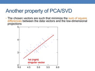
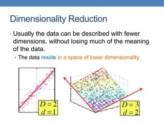
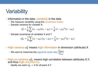
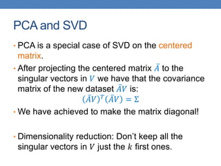
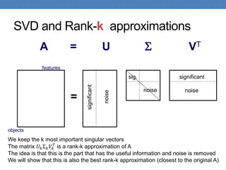
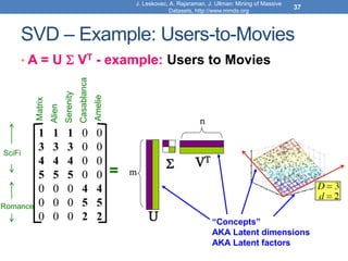
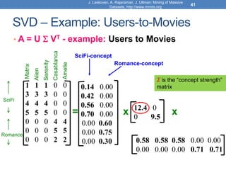
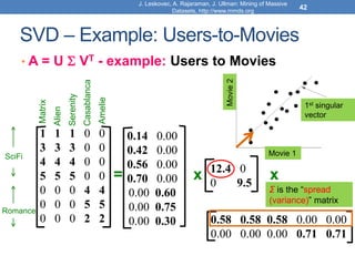
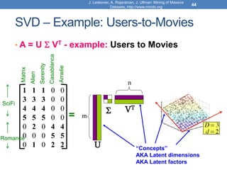
Dimensionality reduction techniques like principal component analysis (PCA) and singular value decomposition (SVD) are important for analyzing high-dimensional data by finding patterns in the data and expressing the data in a lower-dimensional space. PCA and SVD decompose a data matrix into orthogonal principal components/singular vectors that capture the maximum variance in the data, allowing the data to be represented in fewer dimensions without losing much information. Dimensionality reduction is useful for visualization, removing noise, discovering hidden correlations, and more efficiently storing and processing the data.

1. DATA MINING
LECTURE 6
Dimensionality Reduction
PCA – SVD
(Thanks to Jure Leskovec, Evimaria Terzi)

2. The curse of dimensionality
• Real data usually have thousands, or millions of
dimensions
• E.g., web documents, where the dimensionality is the
vocabulary of words
• Facebook graph, where the dimensionality is the
number of users
• Huge number of dimensions causes problems
• Data becomes very sparse, some algorithms become
meaningless (e.g. density based clustering)
• The complexity of several algorithms depends on the
dimensionality and they become infeasible (e.g. nearest
neighbor search).

3. Dimensionality Reduction
• Usually the data can be described with fewer
dimensions, without losing much of the meaning
of the data.
• The data reside in a space of lower dimensionality

4. Example
• In this data matrix the dimension is essentially 3
• There are three types of products and three types of
users
TID A1 A2 A3 A4 A5 A6 A7 A8 A9 A10 B1 B2 B3 B4 B5 B6 B7 B8 B9 B10 C1 C2 C3 C4 C5 C6 C7 C8 C9 C10
1 1 1 1 1 1 1 1 1 1 1 0 0 0 0 0 0 0 0 0 0 0 0 0 0 0 0 0 0 0 0
2 1 1 1 1 1 1 1 1 1 1 0 0 0 0 0 0 0 0 0 0 0 0 0 0 0 0 0 0 0 0
3 1 1 1 1 1 1 1 1 1 1 0 0 0 0 0 0 0 0 0 0 0 0 0 0 0 0 0 0 0 0
4 1 1 1 1 1 1 1 1 1 1 0 0 0 0 0 0 0 0 0 0 0 0 0 0 0 0 0 0 0 0
5 1 1 1 1 1 1 1 1 1 1 0 0 0 0 0 0 0 0 0 0 0 0 0 0 0 0 0 0 0 0
6 0 0 0 0 0 0 0 0 0 0 1 1 1 1 1 1 1 1 1 1 0 0 0 0 0 0 0 0 0 0
7 0 0 0 0 0 0 0 0 0 0 1 1 1 1 1 1 1 1 1 1 0 0 0 0 0 0 0 0 0 0
8 0 0 0 0 0 0 0 0 0 0 1 1 1 1 1 1 1 1 1 1 0 0 0 0 0 0 0 0 0 0
9 0 0 0 0 0 0 0 0 0 0 1 1 1 1 1 1 1 1 1 1 0 0 0 0 0 0 0 0 0 0
10 0 0 0 0 0 0 0 0 0 0 1 1 1 1 1 1 1 1 1 1 0 0 0 0 0 0 0 0 0 0
11 0 0 0 0 0 0 0 0 0 0 0 0 0 0 0 0 0 0 0 0 1 1 1 1 1 1 1 1 1 1
12 0 0 0 0 0 0 0 0 0 0 0 0 0 0 0 0 0 0 0 0 1 1 1 1 1 1 1 1 1 1
13 0 0 0 0 0 0 0 0 0 0 0 0 0 0 0 0 0 0 0 0 1 1 1 1 1 1 1 1 1 1
14 0 0 0 0 0 0 0 0 0 0 0 0 0 0 0 0 0 0 0 0 1 1 1 1 1 1 1 1 1 1
15 0 0 0 0 0 0 0 0 0 0 0 0 0 0 0 0 0 0 0 0 1 1 1 1 1 1 1 1 1 1

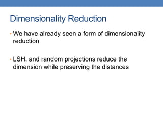
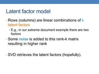
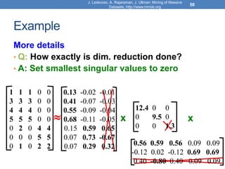
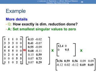
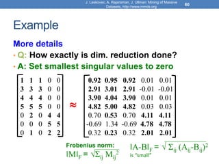
5. Example
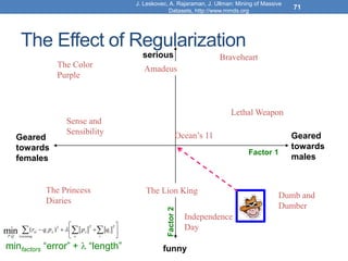
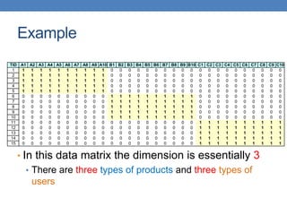
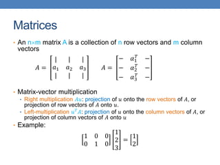
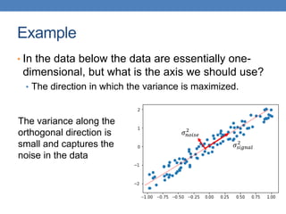
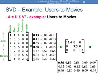
• Cloud of points 3D space:
• Think of point positions
as a matrix:
• We can rewrite coordinates more efficiently!
• Old basis vectors: [1 0 0] [0 1 0] [0 0 1]
• New basis vectors: [1 2 1] [-2 -3 1]
• Then A has new coordinates: [1 0]. B: [0 1], C: [1 -1]
• Notice: We reduced the number of coordinates!
1 row per point:
A
B
C
A
J. Leskovec, A. Rajaraman, J. Ullman: Mining of Massive
Datasets, http://www.mmds.org
5

6. Dimensionality Reduction
• Find the “true dimension” of the data
• In reality things are never as clear and simple as in this
example, but we can still reduce the dimension.
• Essentially, we assume that some of the data is
useful signal and some data is noise, and that we
can approximate the useful part with a lower
dimensionality space.
• Dimensionality reduction does not just reduce the
amount of data, it often brings out the useful part of the
data

7. Dimensionality Reduction
• Goal of dimensionality reduction is to
discover the axis of data!
Rather than representing
every point with 2 coordinates
we represent each point with
1 coordinate (corresponding to
the position of the point on
the red line).
By doing this we incur a bit of
error as the points do not
exactly lie on the line
J. Leskovec, A. Rajaraman, J. Ullman: Mining of Massive
Datasets, http://www.mmds.org
7

8. Why Reduce Dimensions?
• Discover hidden correlations/topics
• E.g., in documents, words that occur commonly
together
• Remove redundant and noisy features
• E.g., in documents, not all words are useful
• Interpretation and visualization
• Easier storage and processing of the data
J. Leskovec, A. Rajaraman, J. Ullman: Mining of Massive
Datasets, http://www.mmds.org
8

9. Dimensionality Reduction
• We have already seen a form of dimensionality
reduction
• LSH, and random projections reduce the
dimension while preserving the distances

10. Data in the form of a matrix
• We are given 𝑛 objects and 𝑑 attributes describing
the objects. Each object has 𝑑 numeric values
describing it.
• We will represent the data as a 𝑛 × 𝑑 real matrix A.
• We can now use tools from linear algebra to process the
data matrix
• Our goal is to produce a new 𝑛 × 𝑘 matrix B such that
• It preserves as much of the information in the original matrix
A as possible
• It reveals something about the structure of the data in A

11. Example: Document matrices
n documents
d terms
(e.g., theorem, proof, etc.)
Aij = frequency of the j-th
term in the i-th document
Find subsets of terms that bring documents
together

12. Example: Recommendation systems
n customers
d movies
Aij = rating of j-th
product by the i-th
customer
Find subsets of movies that capture the
behavior or the customers

13. Linear algebra
• We assume that vectors are column vectors.
• We use 𝑣𝑇 for the transpose of vector 𝑣 (row vector)
• Dot product: 𝑢𝑇𝑣 (1𝑛, 𝑛1 → 11)
• The dot product is the projection of vector 𝑣 on 𝑢 (and vice versa)
• 1, 2, 3
4
1
2
= 12
• 𝑢𝑇𝑣 = 𝑣 𝑢 cos(𝑢, 𝑣)
• If ||𝑢|| = 1 (unit vector) then 𝑢𝑇𝑣 is the projection length of 𝑣 on 𝑢
• −1, 2, 3
4
−1
2
= 0 : orthogonal vectors
• Orthonormal vectors: two unit vectors that are orthogonal

14. Matrices
• An nm matrix A is a collection of n row vectors and m column
vectors
𝐴 =
| | |
𝑎1 𝑎2 𝑎3
| | |
𝐴 =
− 𝛼1
𝑇
−
− 𝛼2
𝑇
−
− 𝛼3
𝑇
−
• Matrix-vector multiplication
• Right multiplication 𝐴𝑢: projection of 𝑢 onto the row vectors of 𝐴, or
projection of row vectors of 𝐴 onto 𝑢.
• Left-multiplication 𝑢𝑇
𝐴: projection of 𝑢 onto the column vectors of 𝐴, or
projection of column vectors of 𝐴 onto 𝑢
• Example:
1 0 0
0 1 0
1
2
3
=
1
2

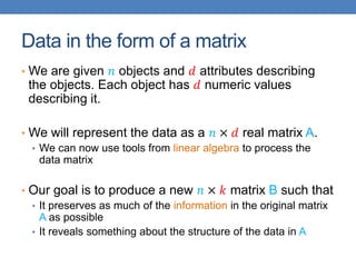
15. Change of basis
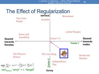
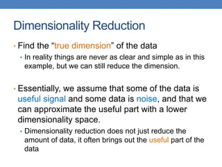
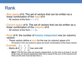
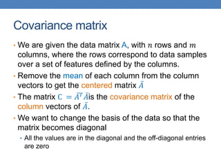
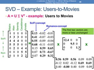
• By default a vector is expressed in the axis-aligned basis.
• For example, for vector [-1,2] we have:
•
−1
2
= −1
1
0
+ 2
0
1
• With a projection we can change the basis over which a
vector is expressed.
√2
2
√2
2
−
√2
2
√2
2
−1
2
=
3√2
2
√2
2

16. Rank
• Row space of A: The set of vectors that can be written as a
linear combination of the rows of A
• All vectors of the form 𝑣 = 𝑢𝑇
𝐴
• Column space of A: The set of vectors that can be written as a
linear combination of the columns of A
• All vectors of the form 𝑣 = 𝐴𝑢.
• Rank of A: the number of linearly independent row (or column)
vectors
• These vectors define a basis for the row (or column) space of A
• All vectors in the row (column) space are linear combinations of the basis vectors
• Example
• Matrix A = has rank r=2
• Why? The first two rows are linearly independent, so the rank is at least 2, but all
three rows are linearly dependent (the first is equal to the sum of the second and
third) so the rank must be less than 3.

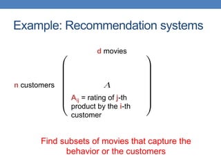
17. Rank-1 matrices
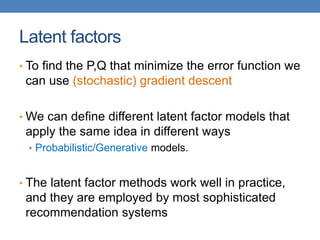
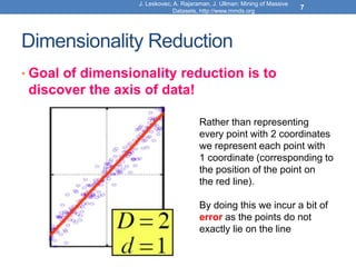
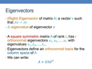
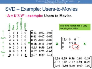
• In a rank-1 matrix, all columns (or rows) are multiples
of the same column (or row) vector
𝐴 =
1 2 −1
2 4 −2
3 6 −3
• All rows are multiples of 𝑟𝑇
= [1,2, −1]
• All columns are multiples of 𝑐 =
1
2
3
• External product: 𝑢𝑣𝑇
(𝑛1 , 1𝑚 → 𝑛𝑚)
• The resulting 𝑛𝑚 has rank 1: all rows (or columns) are
linearly dependent
• 𝐴 = 𝑐𝑟𝑇

18. Eigenvectors
• (Right) Eigenvector of matrix A: a vector v such
that 𝐴𝑣 = 𝜆𝑣
• 𝜆: eigenvalue of eigenvector 𝑣
• A square symmetric matrix A of rank r, has r
orthonormal eigenvectors 𝑢1, 𝑢2, … , 𝑢𝑟 with
eigenvalues 𝜆1, 𝜆2, … , 𝜆𝑟.
• Eigenvectors define an orthonormal basis for the
column space of A
• We can write:
𝐴 = 𝑈Λ𝑈𝑇

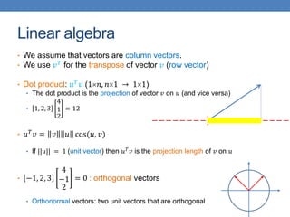
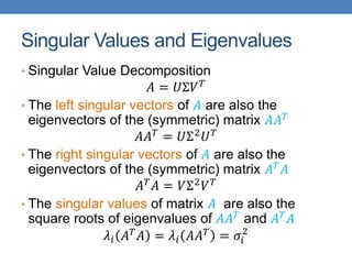
19. Singular Value Decomposition
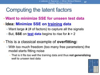
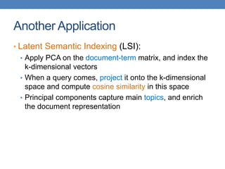
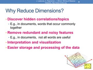
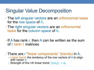
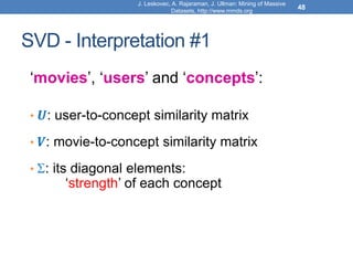
𝐴 = 𝑈 Σ 𝑉𝑇 = 𝑢1, 𝑢2, ⋯ , 𝑢𝑟
𝜎1
𝜎2
0
0
⋱
𝜎𝑟
𝑣1
𝑇
𝑣2
𝑇
⋮
𝑣𝑟
𝑇
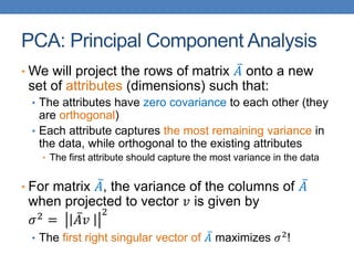
• 𝜎1, ≥ 𝜎2 ≥ ⋯ ≥ 𝜎𝑟: singular values of matrix 𝐴
• 𝑢1, 𝑢2, … , 𝑢𝑟: left singular vectors of 𝐴
• 𝑣1, 𝑣2, … , 𝑣𝑟: right singular vectors of 𝐴
𝐴 = 𝜎1𝑢1𝑣1
𝑇
+ 𝜎2𝑢2𝑣2
𝑇
+ ⋯ + 𝜎𝑟𝑢𝑟𝑣𝑟
𝑇
[n×r] [r×r] [r×m]
r: rank of matrix A
[n×m] =

20. Singular Value Decomposition
• The left singular vectors are an orthonormal basis
for the row space of A.
• The right singular vectors are an orthonormal
basis for the column space of A.
• If A has rank r, then A can be written as the sum
of r rank-1 matrices
• There are r “linear components” (trends) in A.
• Linear trend: the tendency of the row vectors of A to align
with vector v
• Strength of the i-th linear trend: ||𝐴𝒗𝒊|| = 𝝈𝒊

21. Symmetric matrices
• Special case: A is symmetric positive definite
matrix
𝐴 = 𝜆1𝑢1𝑢1
𝑇
+ 𝜆2𝑢2𝑢2
𝑇
+ ⋯ + 𝜆𝑟𝑢𝑟𝑢𝑟
𝑇
• 𝜆1 ≥ 𝜆2 ≥ ⋯ ≥ 𝜆𝑟 ≥ 0: Eigenvalues of A
• 𝑢1, 𝑢2, … , 𝑢𝑟: Eigenvectors of A

22. Singular Values and Eigenvalues
• Singular Value Decomposition
𝐴 = 𝑈Σ𝑉𝑇
• The left singular vectors of 𝐴 are also the
eigenvectors of the (symmetric) matrix 𝐴𝐴𝑇
𝐴𝐴𝑇 = 𝑈Σ2𝑈𝑇
• The right singular vectors of 𝐴 are also the
eigenvectors of the (symmetric) matrix 𝐴𝑇𝐴
𝐴𝑇
𝐴 = 𝑉Σ2
𝑉𝑇
• The singular values of matrix 𝐴 are also the
square roots of eigenvalues of 𝐴𝐴𝑇 and 𝐴𝑇𝐴
𝜆𝑖 𝐴𝑇𝐴 = 𝜆𝑖 𝐴𝐴𝑇 = 𝜎𝑖
2

23. SVD properties
• Singular Value Decomposition has three useful
properties that we will study now:
• It provides the important (principal) directions
(dimensions) in the data – Principal Component
Analysis
• It provides the best low rank approximation for our
matrix
• It minimizes the reconstruction error (squared distance
between real data points and their estimates)

24. Principal Component Analysis
• Goal: reduce the dimensionality while preserving
the “information in the data”.
• In the new space we want to:
• Maximize the amount of information
• Minimize redundancy – remove the redundant
dimensions
• Minimize the noise in the data.

25. Variability
• Information in the data: variability in the data
• We measure variability using the covariance matrix.
• Sample variance for variable X:
𝜎𝑋
2
=
1
𝑁
𝑖
𝑥𝑖 − 𝜇𝑋 𝑥𝑖 − 𝜇𝑋 =
1
𝑁
𝑥 − 𝜇𝑋
𝑇
𝑥 − 𝜇𝑋
• Sample covariance of variables X and Y
𝜎𝑋𝑌
2
=
1
𝑁
𝑖
(𝑥𝑖 − 𝜇𝑋) (𝑦𝑖 − 𝜇𝑌) =
1
𝑁
𝑥 − 𝜇𝑋
𝑇
𝑦 − 𝜇𝑌
• High variance 𝜎𝑋
2
means high information in dimension (attribute) X
• We want to maximize the signal-to-noise ratio
𝜎𝑠𝑖𝑔𝑛𝑎𝑙
2
𝜎𝑛𝑜𝑖𝑠𝑒
2
• High co-variance 𝜎𝑋𝑌
2
means high correlation between attributes X,Y,
and thus high redundancy.
• Ideally we want 𝜎𝑋𝑌
2
= 0 for all pairs X,Y

26. Example
• In the data below the data are essentially one-
dimensional, but what is the axis we should use?
• The direction in which the variance is maximized.
𝜎𝑠𝑖𝑔𝑛𝑎𝑙
2
𝜎𝑛𝑜𝑖𝑠𝑒
2
The variance along the
orthogonal direction is
small and captures the
noise in the data

27. Covariance matrix
• We are given the data matrix A, with 𝑛 rows and 𝑚
columns, where the rows correspond to data samples
over a set of features defined by the columns.
• Remove the mean of each column from the column
vectors to get the centered matrix 𝐴
• The matrix C = 𝐴𝑇
𝐴is the covariance matrix of the
column vectors of 𝐴.
• We want to change the basis of the data so that the
matrix becomes diagonal
• All the values are in the diagonal and the off-diagonal entries
are zero

28. PCA: Principal Component Analysis
• We will project the rows of matrix 𝐴 onto a new
set of attributes (dimensions) such that:
• The attributes have zero covariance to each other (they
are orthogonal)
• Each attribute captures the most remaining variance in
the data, while orthogonal to the existing attributes
• The first attribute should capture the most variance in the data
• For matrix 𝐴, the variance of the columns of 𝐴
when projected to vector 𝑣 is given by
𝜎2
= 𝐴𝑣
2
• The first right singular vector of 𝐴 maximizes 𝜎2!

29. PCA and SVD
• PCA is a special case of SVD on the centered
matrix.
• After projecting the centered matrix 𝐴 to the
singular vectors in 𝑉 we have that the covariance
matrix of the new dataset 𝐴𝑉 is:
𝐴𝑉 𝑇
𝐴𝑉 = Σ
• We have achieved to make the matrix diagonal!
• Dimensionality reduction: Don’t keep all the
singular vectors in 𝑉 just the 𝑘 first ones.

30. 4.0 4.5 5.0 5.5 6.0
2
3
4
5
PCA
Input: 2-d dimensional points
Output:
1st (right)
singular vector
1st (right) singular vector:
direction of maximal variance,
2nd (right)
singular
vector
2nd (right) singular vector:
direction of maximal variance,
after removing the projection of
the data along the first singular
vector.

31. Singular values
1: measures data variance
along the first singular vector.
2: measures how much of the
data variance is explained by
the second singular vector.
1
4.0 4.5 5.0 5.5 6.0
2
3
4
5
1st (right)
singular vector
2nd (right)
singular
vector

32. Singular values tell us something about
the variance
• The variance in the direction of the k-th principal component
is given by the corresponding singular value σk
2
• Singular values can be used to estimate how many
components to keep
• Rule of thumb: keep enough to explain 85% of the
variation:
85
.
0
1
2
1
2





n
j
j
k
j
j



33. A VT

U
=
objects
features
significant
noise
noise
noise
significant
sig.
=
SVD and Rank-k approximations
We keep the k most important singular vectors
The matrix 𝑈𝑘Σ𝑘𝑉𝑘
𝑇
is a rank-k approximation of A
The idea is that this is the part that has the useful information and noise is removed
We will show that this is also the best rank-k approximation (closest to the original A)

34. Example
𝐴 =
𝑎11 ⋯ 𝑎1𝑛
⋮ ⋱ ⋮
𝑎𝑛1 ⋯ 𝑎𝑛𝑛
𝐴 = 𝑈Σ𝑉𝑇
• First right singular vector 𝑣1
• More or less same weight to all drugs
• Discriminates heavy from light users
• Second right singular vector
• Positive values for legal drugs, negative for illegal
students
drugs
legal illegal
𝑎𝑖𝑗: usage of student i of drug j
Drug 2
Drug 1

35. SVD for matrix reconstruction
• We will now see how we can use the fact that
SVD gives the best rank-k approximation for a
data matrix A.
• The idea is that we assume that the “true” matrix
is rank-k, and rank is increased due to noise
• We use SVD to find the best rank-k
approximation for A, and thus the best
approximation of the “true” matrix

36. An (extreme) example
• User-Movie matrix
• Blue and Red rows (colums) are linearly dependent
• There are two prototype users (vectors of movies): blue and
red
• To describe the data is enough to describe the two prototypes, and the
projection weights for each row
• A is a rank-2 matrix
𝐴 = 𝑤1, 𝑤2
𝑑1
𝑇
𝑑2
𝑇
A =

37. SVD – Example: Users-to-Movies
• A = U  VT - example: Users to Movies
J. Leskovec, A. Rajaraman, J. Ullman: Mining of Massive
Datasets, http://www.mmds.org
37
=
SciFi
Romance
Matrix
Alien
Serenity
Casablanca
Amelie
1 1 1 0 0
3 3 3 0 0
4 4 4 0 0
5 5 5 0 0
0 0 0 4 4
0 0 0 5 5
0 0 0 2 2

m
n
U
VT
“Concepts”
AKA Latent dimensions
AKA Latent factors

38. SVD – Example: Users-to-Movies
• A = U  VT - example: Users to Movies
J. Leskovec, A. Rajaraman, J. Ullman: Mining of Massive
Datasets, http://www.mmds.org
38
SciFi-concept
Romance-concept
=
SciFi
Romance
x x
Matrix
Alien
Serenity
Casablanca
Amelie
0.14 0.00
0.42 0.00
0.56 0.00
0.70 0.00
0.00 0.60
0.00 0.75
0.00 0.30
12.4 0
0 9.5
0.58 0.58 0.58 0.00 0.00
0.00 0.00 0.00 0.71 0.71
1 1 1 0 0
3 3 3 0 0
4 4 4 0 0
5 5 5 0 0
0 0 0 4 4
0 0 0 5 5
0 0 0 2 2

39. SVD – Example: Users-to-Movies
• A = U  VT - example: Users to Movies
J. Leskovec, A. Rajaraman, J. Ullman: Mining of Massive
Datasets, http://www.mmds.org
39
SciFi-concept
Romance-concept
=
SciFi
Romance
x x
Matrix
Alien
Serenity
Casablanca
Amelie
0.14 0.00
0.42 0.00
0.56 0.00
0.70 0.00
0.00 0.60
0.00 0.75
0.00 0.30
12.4 0
0 9.5
0.58 0.58 0.58 0.00 0.00
0.00 0.00 0.00 0.71 0.71
1 1 1 0 0
3 3 3 0 0
4 4 4 0 0
5 5 5 0 0
0 0 0 4 4
0 0 0 5 5
0 0 0 2 2
U is “user-to-concept”
similarity matrix

40. SVD – Example: Users-to-Movies
• A = U  VT - example: Users to Movies
J. Leskovec, A. Rajaraman, J. Ullman: Mining of Massive
Datasets, http://www.mmds.org
40
SciFi-concept
Romance-concept
=
SciFi
Romance
x x
Matrix
Alien
Serenity
Casablanca
Amelie
0.14 0.00
0.42 0.00
0.56 0.00
0.70 0.00
0.00 0.60
0.00 0.75
0.00 0.30
12.4 0
0 9.5
0.58 0.58 0.58 0.00 0.00
0.00 0.00 0.00 0.71 0.71
1 1 1 0 0
3 3 3 0 0
4 4 4 0 0
5 5 5 0 0
0 0 0 4 4
0 0 0 5 5
0 0 0 2 2
V is “movie to concept”
similarity matrix

41. SVD – Example: Users-to-Movies
• A = U  VT - example: Users to Movies
J. Leskovec, A. Rajaraman, J. Ullman: Mining of Massive
Datasets, http://www.mmds.org
41
SciFi-concept
Romance-concept
=
SciFi
Romance
x x
Matrix
Alien
Serenity
Casablanca
Amelie
0.14 0.00
0.42 0.00
0.56 0.00
0.70 0.00
0.00 0.60
0.00 0.75
0.00 0.30
12.4 0
0 9.5
0.58 0.58 0.58 0.00 0.00
0.00 0.00 0.00 0.71 0.71
1 1 1 0 0
3 3 3 0 0
4 4 4 0 0
5 5 5 0 0
0 0 0 4 4
0 0 0 5 5
0 0 0 2 2
Σ is the “concept strength”
matrix

42. SVD – Example: Users-to-Movies
• A = U  VT - example: Users to Movies
J. Leskovec, A. Rajaraman, J. Ullman: Mining of Massive
Datasets, http://www.mmds.org
42
=
SciFi
Romance
x x
Matrix
Alien
Serenity
Casablanca
Amelie
0.14 0.00
0.42 0.00
0.56 0.00
0.70 0.00
0.00 0.60
0.00 0.75
0.00 0.30
12.4 0
0 9.5
0.58 0.58 0.58 0.00 0.00
0.00 0.00 0.00 0.71 0.71
1 1 1 0 0
3 3 3 0 0
4 4 4 0 0
5 5 5 0 0
0 0 0 4 4
0 0 0 5 5
0 0 0 2 2
Movie 1
Movie
2
1st singular
vector
Σ is the “spread
(variance)” matrix

43. An (more realistic) example
• User-Movie matrix
• There are two prototype users and movies but
they are noisy
A =

44. SVD – Example: Users-to-Movies
• A = U  VT - example: Users to Movies
J. Leskovec, A. Rajaraman, J. Ullman: Mining of Massive
Datasets, http://www.mmds.org
44
=
SciFi
Romance
Matrix
Alien
Serenity
Casablanca
Amelie
1 1 1 0 0
3 3 3 0 0
4 4 4 0 0
5 5 5 0 0
0 2 0 4 4
0 0 0 5 5
0 1 0 2 2

m
n
U
VT
“Concepts”
AKA Latent dimensions
AKA Latent factors

45. SVD – Example: Users-to-Movies
• A = U  VT - example: Users to Movies
J. Leskovec, A. Rajaraman, J. Ullman: Mining of Massive
Datasets, http://www.mmds.org
45
=
SciFi
Romance
x x
Matrix
Alien
Serenity
Casablanca
Amelie
1 1 1 0 0
3 3 3 0 0
4 4 4 0 0
5 5 5 0 0
0 2 0 4 4
0 0 0 5 5
0 1 0 2 2
0.13 -0.02 -0.01
0.41 -0.07 -0.03
0.55 -0.09 -0.04
0.68 -0.11 -0.05
0.15 0.59 0.65
0.07 0.73 -0.67
0.07 0.29 0.32
12.4 0 0
0 9.5 0
0 0 1.3
0.56 0.59 0.56 0.09 0.09
-0.12 0.02 -0.12 0.69 0.69
0.40 -0.80 0.40 0.09 0.09

46. SVD – Example: Users-to-Movies
• A = U  VT - example: Users to Movies
J. Leskovec, A. Rajaraman, J. Ullman: Mining of Massive
Datasets, http://www.mmds.org
46
=
SciFi
Rom
x x
Matrix
Alien
Serenity
Casablanca
Amelie
1 1 1 0 0
3 3 3 0 0
4 4 4 0 0
5 5 5 0 0
0 2 0 4 4
0 0 0 5 5
0 1 0 2 2
0.13 -0.02 -0.01
0.41 -0.07 -0.03
0.55 -0.09 -0.04
0.68 -0.11 -0.05
0.15 0.59 0.65
0.07 0.73 -0.67
0.07 0.29 0.32
12.4 0 0
0 9.5 0
0 0 1.3
0.56 0.59 0.56 0.09 0.09
-0.12 0.02 -0.12 0.69 0.69
0.40 -0.80 0.40 0.09 0.09
SciFi-concept
Romance-concept
The first two vectors are
more or less unchanged

47. SVD – Example: Users-to-Movies
• A = U  VT - example: Users to Movies
J. Leskovec, A. Rajaraman, J. Ullman: Mining of Massive
Datasets, http://www.mmds.org
47
=
SciFi
Rom
x x
Matrix
Alien
Serenity
Casablanca
Amelie
1 1 1 0 0
3 3 3 0 0
4 4 4 0 0
5 5 5 0 0
0 2 0 4 4
0 0 0 5 5
0 1 0 2 2
0.13 -0.02 -0.01
0.41 -0.07 -0.03
0.55 -0.09 -0.04
0.68 -0.11 -0.05
0.15 0.59 0.65
0.07 0.73 -0.67
0.07 0.29 0.32
12.4 0 0
0 9.5 0
0 0 1.3
0.56 0.59 0.56 0.09 0.09
-0.12 0.02 -0.12 0.69 0.69
0.40 -0.80 0.40 0.09 0.09
The third vector has a very
low singular value

48. J. Leskovec, A. Rajaraman, J. Ullman: Mining of Massive
Datasets, http://www.mmds.org
48
SVD - Interpretation #1
‘movies’, ‘users’ and ‘concepts’:
• 𝑼: user-to-concept similarity matrix
• 𝑽: movie-to-concept similarity matrix
• : its diagonal elements:
‘strength’ of each concept

49. Rank-k approximation
• In this User-Movie matrix
• We have more than two singular vectors, but the
strongest ones are still about the two types.
• The third models the noise in the data
• By keeping the two strongest singular vectors we
obtain most of the information in the data.
• This is a rank-2 approximation of the matrix A
A =

50. Rank-k approximations (Ak)
𝑼𝒌 (𝑽𝒌): orthogonal matrix containing the top k left (right)
singular vectors of A.
𝜮𝒌: diagonal matrix containing the top k singular values of A
Ak is an approximation of A
n x d n x k k x k k x d
Ak is the best approximation of A

51. SVD as an optimization
• The rank-k approximation matrix 𝐴𝑘 produced by
the top-k singular vectors of A minimizes the
Frobenious norm of the difference with the matrix A
𝐴𝑘 = arg max
𝐵:𝑟𝑎𝑛𝑘 𝐵 =𝑘
𝐴 − 𝐵 𝐹
2
𝐴 − 𝐵 𝐹
2
=
𝑖,𝑗
𝐴𝑖𝑗 − 𝐵𝑖𝑗
2
Explanation: The (𝑖, 𝑗) cell in 𝐴𝑘is close on average with the 𝑖, 𝑗 cell of 𝐴

52. What does this mean?
• We can project the row (and column) vectors of
the matrix A into a k-dimensional space and
preserve most of the information
• (Ideally) The k dimensions reveal latent
features/aspects/topics of the term (document)
space.
• (Ideally) The 𝐴𝑘 approximation of matrix A,
contains all the useful information, and what is
discarded is noise

53. Latent factor model
• Rows (columns) are linear combinations of k
latent factors
• E.g., in our extreme document example there are two
factors
• Some noise is added to this rank-k matrix
resulting in higher rank
• SVD retrieves the latent factors (hopefully).

54. A VT

U
=
objects
features
significant
noise
noise
noise
significant sig.
=
SVD and Rank-k approximations

55. Example
More details
• Q: How exactly is dim. reduction done?
• A: Compute SVD
J. Leskovec, A. Rajaraman, J. Ullman: Mining of Massive
Datasets, http://www.mmds.org
55
= x x
1 1 1 0 0
3 3 3 0 0
4 4 4 0 0
5 5 5 0 0
0 2 0 4 4
0 0 0 5 5
0 1 0 2 2
12.4 0 0
0 9.5 0
0 0 1.3
0.13 -0.02 -0.01
0.41 -0.07 -0.03
0.55 -0.09 -0.04
0.68 -0.11 -0.05
0.15 0.59 0.65
0.07 0.73 -0.67
0.07 0.29 0.32 0.56 0.59 0.56 0.09 0.09
-0.12 0.02 -0.12 0.69 0.69
0.40 -0.80 0.40 0.09 0.09

56. Example
More details
• Q: How exactly is dim. reduction done?
• A: Set smallest singular values to zero
J. Leskovec, A. Rajaraman, J. Ullman: Mining of Massive
Datasets, http://www.mmds.org
56
= x x
1 1 1 0 0
3 3 3 0 0
4 4 4 0 0
5 5 5 0 0
0 2 0 4 4
0 0 0 5 5
0 1 0 2 2
12.4 0 0
0 9.5 0
0 0 1.3
0.13 -0.02 -0.01
0.41 -0.07 -0.03
0.55 -0.09 -0.04
0.68 -0.11 -0.05
0.15 0.59 0.65
0.07 0.73 -0.67
0.07 0.29 0.32 0.56 0.59 0.56 0.09 0.09
-0.12 0.02 -0.12 0.69 0.69
0.40 -0.80 0.40 0.09 0.09

57. Example
More details
• Q: How exactly is dim. reduction done?
• A: Set smallest singular values to zero
J. Leskovec, A. Rajaraman, J. Ullman: Mining of Massive
Datasets, http://www.mmds.org
57
x x
1 1 1 0 0
3 3 3 0 0
4 4 4 0 0
5 5 5 0 0
0 2 0 4 4
0 0 0 5 5
0 1 0 2 2
12.4 0 0
0 9.5 0
0 0 1.3

0.13 -0.02 -0.01
0.41 -0.07 -0.03
0.55 -0.09 -0.04
0.68 -0.11 -0.05
0.15 0.59 0.65
0.07 0.73 -0.67
0.07 0.29 0.32 0.56 0.59 0.56 0.09 0.09
-0.12 0.02 -0.12 0.69 0.69
0.40 -0.80 0.40 0.09 0.09

58. Example
More details
• Q: How exactly is dim. reduction done?
• A: Set smallest singular values to zero
J. Leskovec, A. Rajaraman, J. Ullman: Mining of Massive
Datasets, http://www.mmds.org
58
x x
1 1 1 0 0
3 3 3 0 0
4 4 4 0 0
5 5 5 0 0
0 2 0 4 4
0 0 0 5 5
0 1 0 2 2
12.4 0 0
0 9.5 0
0 0 1.3

0.13 -0.02 -0.01
0.41 -0.07 -0.03
0.55 -0.09 -0.04
0.68 -0.11 -0.05
0.15 0.59 0.65
0.07 0.73 -0.67
0.07 0.29 0.32 0.56 0.59 0.56 0.09 0.09
-0.12 0.02 -0.12 0.69 0.69
0.40 -0.80 0.40 0.09 0.09

59. Example
More details
• Q: How exactly is dim. reduction done?
• A: Set smallest singular values to zero
J. Leskovec, A. Rajaraman, J. Ullman: Mining of Massive
Datasets, http://www.mmds.org
59
 x x
1 1 1 0 0
3 3 3 0 0
4 4 4 0 0
5 5 5 0 0
0 2 0 4 4
0 0 0 5 5
0 1 0 2 2
12.4 0
0 9.5
0.13 -0.02
0.41 -0.07
0.55 -0.09
0.68 -0.11
0.15 0.59
0.07 0.73
0.07 0.29 0.56 0.59 0.56 0.09 0.09
-0.12 0.02 -0.12 0.69 0.69

60. Example
More details
• Q: How exactly is dim. reduction done?
• A: Set smallest singular values to zero
J. Leskovec, A. Rajaraman, J. Ullman: Mining of Massive
Datasets, http://www.mmds.org
60

1 1 1 0 0
3 3 3 0 0
4 4 4 0 0
5 5 5 0 0
0 2 0 4 4
0 0 0 5 5
0 1 0 2 2
0.92 0.95 0.92 0.01 0.01
2.91 3.01 2.91 -0.01 -0.01
3.90 4.04 3.90 0.01 0.01
4.82 5.00 4.82 0.03 0.03
0.70 0.53 0.70 4.11 4.11
-0.69 1.34 -0.69 4.78 4.78
0.32 0.23 0.32 2.01 2.01
Frobenius norm:
ǁMǁF = Σij Mij
2
ǁA-BǁF =  Σij (Aij-Bij)2
is “small”

61. Application: Recommender systems
• Data: Users rating movies
• Sparse and often noisy
• Assumption: There are k basic user profiles, and
each user is a linear combination of these profiles
• E.g., action, comedy, drama, romance
• Each user is a weighted combination of these profiles
• The “true” matrix has rank k
• If we had the matrix A with all ratings of all users
for all movies, the matrix 𝐴𝑘 would tell us the true
preferences of the users for the movies

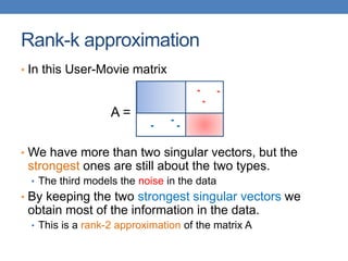
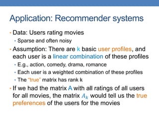
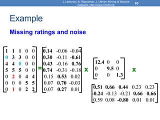
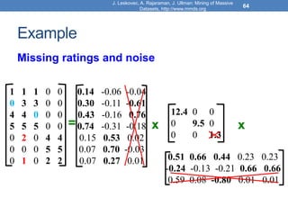
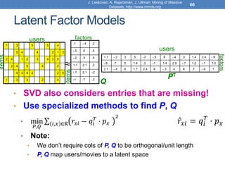
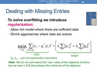
62. Model-based Recommendation Systems
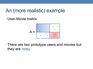
• What we observe is a noisy, and incomplete
version of this matrix 𝐴 ̃
• Given matrix 𝐴 and we would like to get the
missing ratings that 𝐴𝑘 would produce
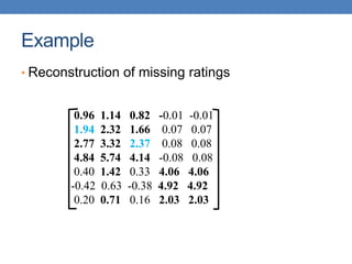
• Algorithm: compute the rank-k approximation 𝐴𝑘
of and matrix 𝐴 predict for user 𝑢 and movie 𝑚,
the value 𝐴𝑘[𝑚, 𝑢].
• The rank-k approximation 𝐴𝑘 is provably close to 𝐴𝑘
• Model-based collaborative filtering

63. Example
Missing ratings and noise
J. Leskovec, A. Rajaraman, J. Ullman: Mining of Massive
Datasets, http://www.mmds.org
63
= x x
1 1 1 0 0
0 3 3 0 0
4 4 0 0 0
5 5 5 0 0
0 2 0 4 4
0 0 0 5 5
0 1 0 2 2
0.14 -0.06 -0.04
0.30 -0.11 -0.61
0.43 -0.16 0.76
0.74 -0.31 -0.18
0.15 0.53 0.02
0.07 0.70 -0.03
0.07 0.27 0.01
12.4 0 0
0 9.5 0
0 0 1.3
0.51 0.66 0.44 0.23 0.23
-0.24 -0.13 -0.21 0.66 0.66
0.59 0.08 -0.80 0.01 0.01

64. Example
Missing ratings and noise
J. Leskovec, A. Rajaraman, J. Ullman: Mining of Massive
Datasets, http://www.mmds.org
64
= x x
1 1 1 0 0
0 3 3 0 0
4 4 0 0 0
5 5 5 0 0
0 2 0 4 4
0 0 0 5 5
0 1 0 2 2
0.14 -0.06 -0.04
0.30 -0.11 -0.61
0.43 -0.16 0.76
0.74 -0.31 -0.18
0.15 0.53 0.02
0.07 0.70 -0.03
0.07 0.27 0.01
12.4 0 0
0 9.5 0
0 0 1.3
0.51 0.66 0.44 0.23 0.23
-0.24 -0.13 -0.21 0.66 0.66
0.59 0.08 -0.80 0.01 0.01

65. Example
• Reconstruction of missing ratings
0.96 1.14 0.82 -0.01 -0.01
1.94 2.32 1.66 0.07 0.07
2.77 3.32 2.37 0.08 0.08
4.84 5.74 4.14 -0.08 0.08
0.40 1.42 0.33 4.06 4.06
-0.42 0.63 -0.38 4.92 4.92
0.20 0.71 0.16 2.03 2.03

66. Latent Factor Models
• SVD also considers entries that are missing!
• Use specialized methods to find P, Q
• min
𝑃,𝑄 𝑖,𝑥 ∈R 𝑟𝑥𝑖 − 𝑞𝑖
𝑇
⋅ 𝑝𝑥
2
• Note:
• We don’t require cols of P, Q to be orthogonal/unit length
• P, Q map users/movies to a latent space
J. Leskovec, A. Rajaraman, J. Ullman: Mining of Massive
Datasets, http://www.mmds.org
66
4
5
5
3
1
3
1
2
4
4
5
5
3
4
3
2
1
4
2
2
4
5
4
2
5
2
2
4
3
4
4
2
3
3
1
.2
-.4
.1
.5
.6
-.5
.5
.3
-.2
.3
2.1
1.1
-2
2.1
-.7
.3
.7
-1
-.9
2.4
1.4
.3
-.4
.8
-.5
-2
.5
.3
-.2
1.1
1.3
-.1
1.2
-.7
2.9
1.4
-1
.3
1.4
.5
.7
-.8
.1
-.6
.7
.8
.4
-.3
.9
2.4
1.7
.6
-.4
2.1

PT
Q
users
items
𝑟𝑥𝑖 = 𝑞𝑖
𝑇
⋅ 𝑝𝑥
factors
factors
items
users

67. Computing the latent factors
• Want to minimize SSE for unseen test data
• Idea: Minimize SSE on training data
• Want large k (# of factors) to capture all the signals
• But, SSE on test data begins to rise for k > 2
• This is a classical example of overfitting:
• With too much freedom (too many free parameters) the
model starts fitting noise
• That is it fits too well the training data and thus not generalizing
well to unseen test data
67
1 3 4
3 5 5
4 5 5
3
3
2 ? ?
?
2 1 ?
3 ?
1
J. Leskovec, A. Rajaraman, J. Ullman: Mining of Massive
Datasets, http://www.mmds.org

68. Dealing with Missing Entries
• To solve overfitting we introduce
regularization:
• Allow rich model where there are sufficient data
• Shrink aggressively where data are scarce
68








 

 i
i
x
x
training
x
T
i
xi
Q
P
q
p
p
q
r
2
2
2
1
2
,
)
(
min 

1 3 4
3 5 5
4 5 5
3
3
2 ? ?
?
2 1 ?
3 ?
1
1, 2 … user set regularization parameters
“error” “length”
Note: We do not care about the “raw” value of the objective function,
but we care in P,Q that achieve the minimum of the objective
J. Leskovec, A. Rajaraman, J. Ullman: Mining of Massive
Datasets, http://www.mmds.org

69. Geared
towards
females
Geared
towards
males
serious
funny
The Effect of Regularization
69
J. Leskovec, A. Rajaraman, J. Ullman: Mining of Massive
Datasets, http://www.mmds.org
The Princess
Diaries
The Lion King
Braveheart
Lethal Weapon
Independence
Day
Amadeus
The Color
Purple
Dumb and
Dumber
Ocean’s 11
Sense and
Sensibility
Factor 1
Factor
2
minfactors “error” +  “length”








 

 i
i
x
x
training
x
i
xi
Q
P
q
p
p
q
r
2
2
2
,
)
(
min 

70. Geared
towards
females
Geared
towards
males
serious
funny
The Effect of Regularization
70
J. Leskovec, A. Rajaraman, J. Ullman: Mining of Massive
Datasets, http://www.mmds.org
The Lion King
Braveheart
Lethal Weapon
Independence
Day
Amadeus
The Color
Purple
Dumb and
Dumber
Ocean’s 11
Sense and
Sensibility
Factor 1
Factor
2
The Princess
Diaries
minfactors “error” +  “length”








 

 i
i
x
x
training
x
i
xi
Q
P
q
p
p
q
r
2
2
2
,
)
(
min 

71. Geared
towards
females
Geared
towards
males
serious
funny
The Effect of Regularization
71
J. Leskovec, A. Rajaraman, J. Ullman: Mining of Massive
Datasets, http://www.mmds.org
The Lion King
Braveheart
Lethal Weapon
Independence
Day
Amadeus
The Color
Purple
Dumb and
Dumber
Ocean’s 11
Sense and
Sensibility
Factor 1
Factor
2
minfactors “error” +  “length”
The Princess
Diaries








 

 i
i
x
x
training
x
i
xi
Q
P
q
p
p
q
r
2
2
2
,
)
(
min 

72. Geared
towards
females
Geared
towards
males
serious
funny
The Effect of Regularization
72
J. Leskovec, A. Rajaraman, J. Ullman: Mining of Massive
Datasets, http://www.mmds.org
The Lion King
Braveheart
Lethal Weapon
Independence
Day
Amadeus
The Color
Purple
Dumb and
Dumber
Ocean’s 11
Sense and
Sensibility
Factor 1
Factor
2
The Princess
Diaries
minfactors “error” +  “length”








 

 i
i
x
x
training
x
i
xi
Q
P
q
p
p
q
r
2
2
2
,
)
(
min 

73. Latent factors
• To find the P,Q that minimize the error function we
can use (stochastic) gradient descent
• We can define different latent factor models that
apply the same idea in different ways
• Probabilistic/Generative models.
• The latent factor methods work well in practice,
and they are employed by most sophisticated
recommendation systems

74. Another Application
• Latent Semantic Indexing (LSI):
• Apply PCA on the document-term matrix, and index the
k-dimensional vectors
• When a query comes, project it onto the k-dimensional
space and compute cosine similarity in this space
• Principal components capture main topics, and enrich
the document representation

75. Another property of PCA/SVD
• The chosen vectors are such that minimize the sum of square
differences between the data vectors and the low-dimensional
projections
4.0 4.5 5.0 5.5 6.0
2
3
4
5
1st (right)
singular vector

76. SVD is “the Rolls-Royce and the Swiss
Army Knife of Numerical Linear
Algebra.”*
*Dianne O’Leary, MMDS ’06

77. Computation of eigenvectors
• Consider a symmetric square matrix 𝑀
• Power-method:
• Start with the vector 𝑣 of all 1’s
• Compute 𝑣 = 𝑀𝑣
• Normalize by the length of 𝑣
• Repeat until the vector does not change
• This will give us the first eigenvector.
• The first eigenvalue is 𝜆 = 𝑣𝑇
𝑀𝑣
• For the second one, compute the first eigenvector of
the matrix 𝑀∗
= 𝑀 − 𝜆𝑣𝑣𝑇

78. Singular Values and Eigenvalues
• The left singular vectors of 𝐴 are also the
eigenvectors of 𝐴𝐴𝑇
• The right singular vectors of 𝐴 are also the
eigenvectors of 𝐴𝑇
𝐴
• The singular values of matrix 𝐴 are also the
square roots of eigenvalues of 𝐴𝐴𝑇 and 𝐴𝑇𝐴

79. Computing singular vectors
• Compute the eigenvectors and eigenvalues of the
matrices 𝑀𝑀𝑇 and 𝑀𝑇𝑀