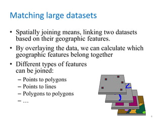
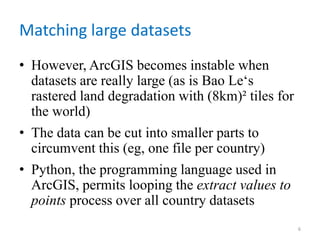
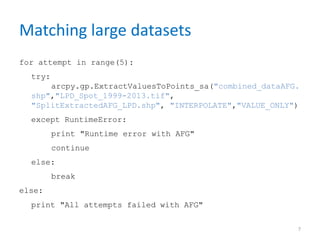
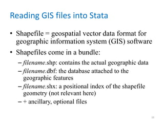
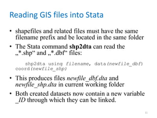
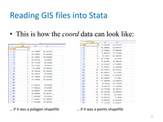
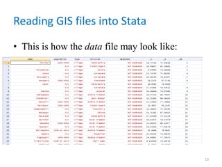
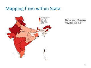
This document discusses several empirical approaches for analyzing large geographic datasets: 1) Matching datasets in ArcGIS by spatially joining points and polygons using tools like Extract Values to Points for large raster datasets. 2) Reading shapefile and database files into Stata using the shp2dta command to link geographic and attribute information. 3) Comparing the costs of action vs. inaction in biomodeling by predicting outcomes under different land management scenarios. 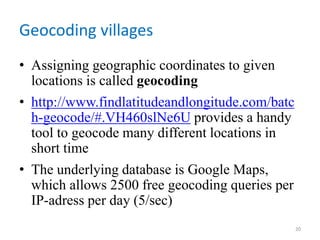4) Geocoding villages without geographic coordinates using online tools to assign latitude and longitude for merging external geographic data. 5) Standardizing country names in Stata using the kountry command to facilitate linking datasets based on country information.

1. Economics of Land Degradation and
Improvement
Jann Goedecke
ZEF Interdisciplinary Course 2014

2. 4. Empirical approaches
1. Matching large datasets based on geographical
information in ArcGIS
2. Reading GIS files into Stata
3. Cost of action vs cost of inaction – the
biomodelling approach
4. Geocoding villages
5. Stata‘s kountry command
2

3. 1. Matching large datasets
based on geographical
information in ArcGIS
3

4. Matching large datasets
• Spatially joining means, linking two datasets
based on their geographic features.
• By overlaying the data, we can calculate which
geographic features belong together
• Different types of features
can be joined:
– Points to polygons
– Points to lines
– Polygons to polygons
– …
4

5. Matching large datasets
• Often, we want to join point information to
geographic polygons
• Points are usually stored in shapefiles
• Polygons, however, are sometimes stored as
raster data (i.e. in quadratic tiles), sometimes
also as shapefiles
• ArcGIS provides tools for either way:
– Extract values to points does the job with rasters
– Spatial join with option „points to polygons“ is
suitable for shapefiles
5

6. Matching large datasets
• However, ArcGIS becomes instable when
datasets are really large (as is Bao Le‘s
rastered land degradation with (8km)² tiles for
the world)
• The data can be cut into smaller parts to
circumvent this (eg, one file per country)
• Python, the programming language used in
ArcGIS, permits looping the extract values to
points process over all country datasets
6

7. Matching large datasets
for attempt in range(5):
try:
arcpy.gp.ExtractValuesToPoints_sa("combined_dataAFG.
shp","LPD_Spot_1999-2013.tif",
"SplitExtractedAFG_LPD.shp", "INTERPOLATE","VALUE_ONLY")
except RuntimeError:
print "Runtime error with AFG"
continue
else:
break
else:
print "All attempts failed with AFG"
7

8. Matching large datasets
for attempt in range(5):
try:
arcpy.gp.ExtractValuesToPoints_sa("combined_dataBRA.
shp","LPD_Spot_1999-2013.tif",
"SplitExtractedBRA_LPD.shp", "INTERPOLATE","VALUE_ONLY")
except RuntimeError:
print "Runtime error with BRA"
continue
else:
break
else:
print "All attempts failed with BRA"
8

9. 2. Reading GIS files into Stata
9

10. Reading GIS files into Stata
• Shapefile = geospatial vector data format for
geographic information system (GIS) software
• Shapefiles come in a bundle:
– filename.shp: contains the actual geographic data
– filename.dbf: the database attached to the
geographic features
– filename.shx: a positional index of the shapefile
geometry (not relevant here)
– + ancillary, optional files
10

11. Reading GIS files into Stata
• shapefiles and related files must have the same
filename prefix and be located in the same folder
• The Stata command shp2dta can read the
„*.shp“ and „*.dbf“ files:
shp2dta using filename, data(newfile_dbf)
coord(newfile_shp)
• This produces files newfile_dbf.dta and
newfile_shp.dta in current working folder
• Both created datasets now contain a new variable
_ID through which they can be linked.
11

12. Reading GIS files into Stata
• This is how the coord data can look like:
12
… if it was a polygon shapefile … if it was a points shapefile

13. Reading GIS files into Stata
• This is how the data file may look like:
13

14. Mapping from within Stata
• The user-written command spmap allows to
map with Stata‘s graph features
• See Maurizio Pisati‘s excellent presentation
for more information
• Be aware that both commands need to be
installed first
14

15. Mapping from within Stata
15
The product of spmap
may look like this

16. 2. Cost of action vs cost of
inaction – the biomodelling
approach
16

17. Cost of action vs cost of inaction – the
biomodelling approach
• Biomodeled data predicts outcomes for a given pixel for different scenarios:
– Irrigated vs rainfed
– ISFM vs business as usual land management
– Type of crop grown
– Year (next 40)
Variables of interest:
– LD costs, component 1: future costs of not switching to ISFM today in degraded areas
– LD costs, component 2: productivity decline in areas already under ISFM due to external
factors
– Total co2 sequest: loss: future value of foregone carbon sequestration due to not switching to
ISFM today in degraded areas
– Co2 sequestration loss isfm: lost value of carbon sequestration in areas already under ISFM due
to external factors
• C:UsersjgoedeckeDropboxZEFIndia Review PaperStata_filesJawoo_costs.do
17

18. 4. Geocoding villages
18

19. Geocoding villages
• Sometimes our initial dataset originates from a
survey where no GIS information has been
collected
• But usually the state, district, and village is
documented
• Ideally, we would like to merge (external)
geographic data (such as land characteristics)
to our main data
19

20. Geocoding villages
• Assigning geographic coordinates to given
locations is called geocoding
• http://www.findlatitudeandlongitude.com/batc
h-geocode/#.VH460slNe6U provides a handy
tool to geocode many different locations in
short time
• The underlying database is Google Maps,
which allows 2500 free geocoding queries per
IP-adress per day (5/sec)
20

21. Geocoding villages
• Another tool developed by researchers from
University of Tokyo in a large scale project is the
India place finder: http://india.csis.u-tokyo.ac.jp/csvmode
• Unique and very powerful, since information was
gathered from many different sources
• They also created a „global place finder“, which
is, however, only based on Google Maps. So there
is probably not much added value to longitude
and latitude finder.
21

22. 5. Stata‘s kountry command
22

23. Stata‘s kountry command
• Back to Stata: if we deal with world-wide data,
at some point we usually encounter issues of
linking datasets based on country information
• Unfortunately, countries have a range of
possible names under which they are stored
– Russia / Russian Federation
– Cote d‘Ivoire / Ivory Coast
– Iran / Islamic Republic of Iran
– …
23

24. Stata‘s kountry command
• Thus we need standardized names to link datasets
based on country names
• Another user-written tool, kountry, is helpful
kountry kountryvar, from(other)
stuck
• That generates a new (numeric) standardized
variable called _ISO3N_
24

25. Stata‘s kountry command
• This, in turn, can be recoded into well-known
formats such as the World Bank ISO codes:
• kountry iso3n, from(iso3n) to(iso3c)
• which creates the variable _ISO3C_, as issued
by the World Bank.
• Other common formats are possible as well.
Check
25

26. 26