Downloaded 24 times


![!25
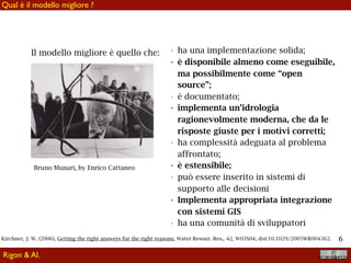
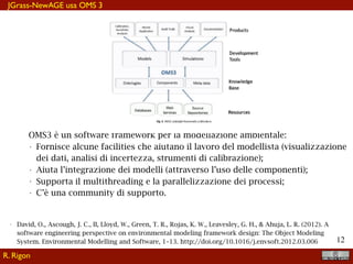
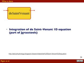
A - AGEs
To be checked
B- JGrass-NewAGE (https://github.com/geoframecomponents)
[Adige]
BP- Backward probabilities
Clearness Index
ET
FP -Forward probabilities
[Kriging]
NetRadiation
LWRB -
RainSnow
SWB (Simple Water Budget)
SWRB
Snow
C - JGrassTools (http://moovida.github.io/jgrasstools/)
More than 50 components
An index
Rigon et al.](https://image.slidesharecdn.com/3-jgrass-newage-170222165449/85/3-j-grass-new-age-25-320.jpg)
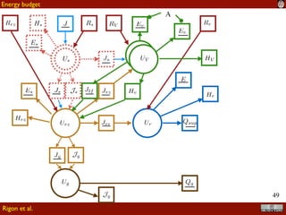
![!28
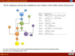
(4.1)
@t
= Jk(t)+
i
Qki(t)° ETk(t)°Qk(t)
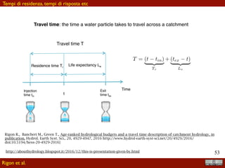
for an appropriate set of elementary control volumes connected together. In Eq.(5.1),
S [L3
] represents the total water storage of the basin, J [L3
T°1
], ET [L3
T°1
], and Q
[L3
T°1
] are precipitation, evapotranspiration, and runoff (surface and groundwater)
respectively. The Qis represent input fluxes, of the same nature of Q, coming from
adjacent control volumes.
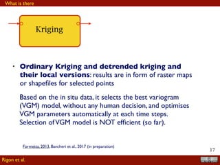
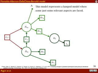
a
b
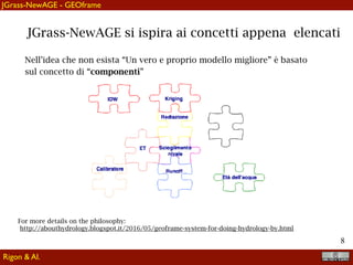
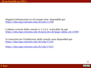
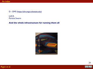
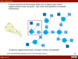
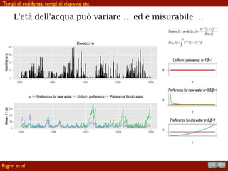
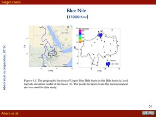
Figure 4.1: The location of the Posina basin in the Northeast of Italy (a) and DEM elava-
tion, location of rain gauges and hydrometer stations, subbasin-channel link partitions
used for this modelling (b).
It is clear that Eq.(5.1) is governed by two types of terms, which can be easily identi-
fied as “inputs" and “outputs". The outputs are certainly evapotranspiration, ET, and
discharges, Q, including the Qis, because they come from the assembly of control volumes.
The inputs are J(t), but this term has to be split into rainfall and snowfall. Moreover,
other inputs are ancillary to the estimation of outputs, in particular temperature, T and
radiation Rn. Another input of the equation is the definition of the domain of integration
and its“granularity", i.e. its partition into elements for which a singe value of the state
variables is produced.
In this paper we discuss the estimation of all of these input quantities, with the
Posina
A small (114 km2) basin in Vicenza province,
flowing into the Brenta river
Abera et al.
A small basin
Abera, 2017](https://image.slidesharecdn.com/3-jgrass-newage-170222165449/85/3-j-grass-new-age-28-320.jpg)

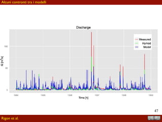
![!48
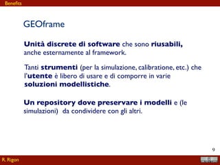
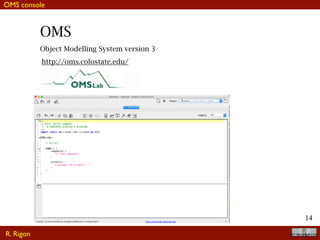
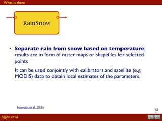
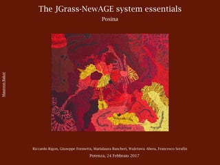
0
50
100
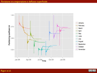
Oct 01 Oct 15 Nov 01 Nov 15 Dec 01 Dec 15
Time [h]
Q[m3
/s]
Measured
Hymod
Model
Discharge peak
Rigon et al.](https://image.slidesharecdn.com/3-jgrass-newage-170222165449/85/3-j-grass-new-age-48-320.jpg)

![!60
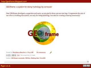
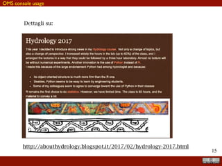
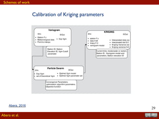
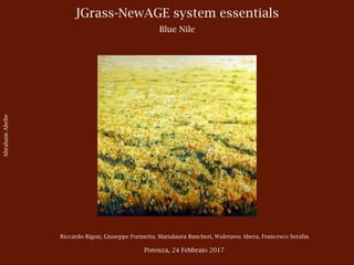
CMORPH is better in estimating ground-gauge rainfall using the two previous statistics
(i.e., r and RMSE), it is underestimating by 72%, thus being the most biased product of
the five SREs. This could be because CMORPH is only based on satellite products, and
not corrected using ground data as 3B42V7. TAMSAT, on average, is underestimating
rainfall by 30%.
CorrelationRMSEBIAS 3B42V7 CMORPH CFSR SM2R-CCI TAMSAT
8
9
10
11
12
13Lat
Correlation
<0.2
(0.2,0.3]
(0.3,0.4]
(0.4,0.5]
(0.5,0.6]
(0.6,0.7]
8
9
10
11
12
13
Lat
RMSE(mm/day)
[4, 6]
(6, 8]
(8, 10]
(10, 12]
(12, 14]
>14
8
9
10
11
12
13
36 38 40 36 38 40 36 38 40 36 38 40 36 38 40
Long
Lat
BIAS
(-0.9,-0.6]
(-0.6,-0.3]
(-0.3,-0.1]
(-0.1,0.1]
(0.1,0.3]
(0.3,0.6]
(0.6,1.4]
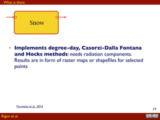
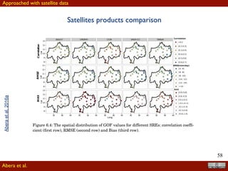
Figure 6.4: The spatial distribution of GOF values for different SREs: correlation coeffi-
cient (first row), RMSE (second row) and Bias (third row).
The spatial distribution of the the three GOF values (r, RMSE, BIAS) are presented
in figure 6.4. Overall the distribution of the statistics can depict a spatial pattern, i.e., the
correlations in the eastern and northeastern part of the basin are higher than western
and southwestern part. Similar pattern can be inferred from the RMSE and BIAS
Satellites products comparison
Abera et al.
Approached with satellite data
Aberaetal,2016](https://image.slidesharecdn.com/3-jgrass-newage-170222165449/85/3-j-grass-new-age-60-320.jpg)
![!67
JGRASS-NEWAGE MODEL SYSTEM AND SATELLITE DATA
0
100
200
Precip[mm/month]
−100
0
100
01 02 03 04 05 06 07 08 09 10 11 12
Months
Fluxes(Q,ET,S)[mm/month]
ET
Q
S
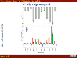
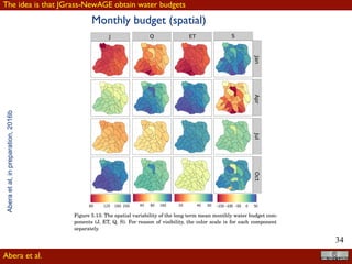
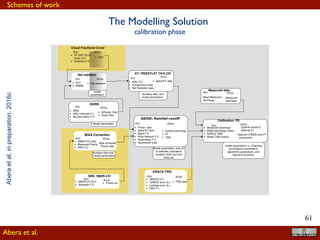
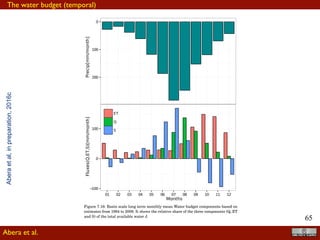
Figure 7.16: Basin scale long term monthly mean Water budget components based on
estimates from 1994 to 2009. It shows the relative share of the three components (Q, ET
and S) of the total available water J.
160
Abera et al.
The water budget (temporal)
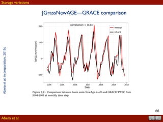
Aberaetal,inreview,2016c](https://image.slidesharecdn.com/3-jgrass-newage-170222165449/85/3-j-grass-new-age-67-320.jpg)


JGrass-NewAge is a modular hydrological modeling system using an object modeling system (OMS) infrastructure that allows for component-based construction of models in Java. It supports various hydrological tasks including discharge calculations, radiation assessment, and water tracer concentration computations, with an emphasis on modern and extensible hydrology. The system enables easy integration with existing software and provides tools for calibration and parallelization, making it adaptable for diverse hydrological studies.


