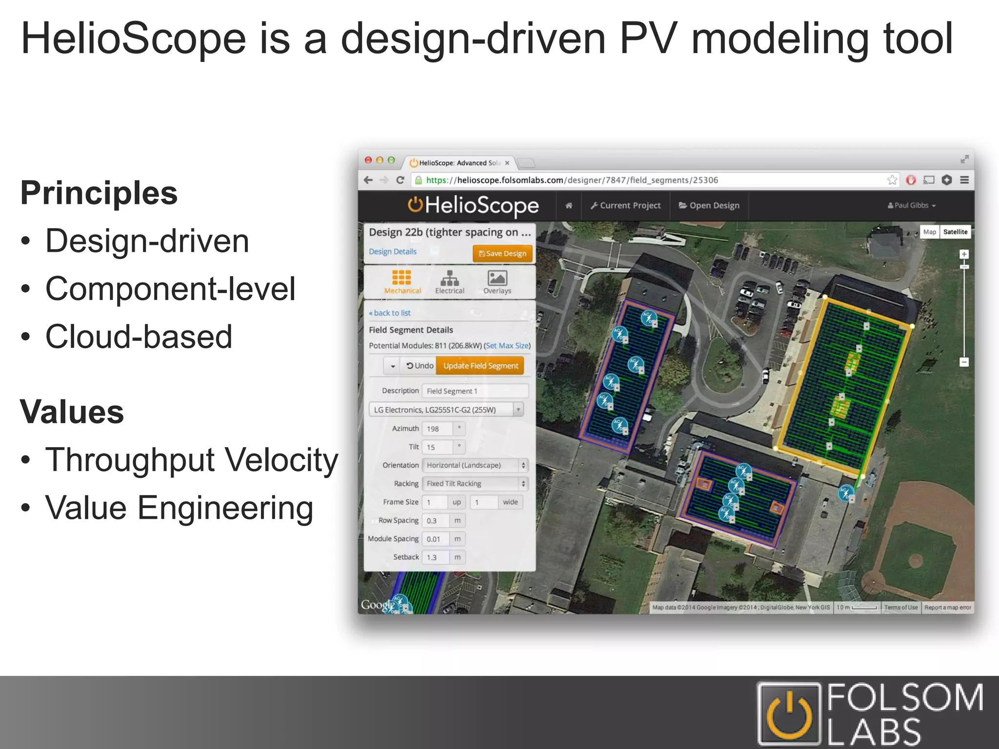
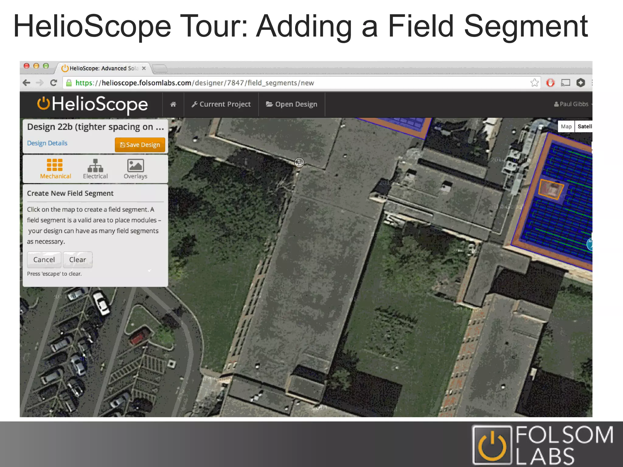
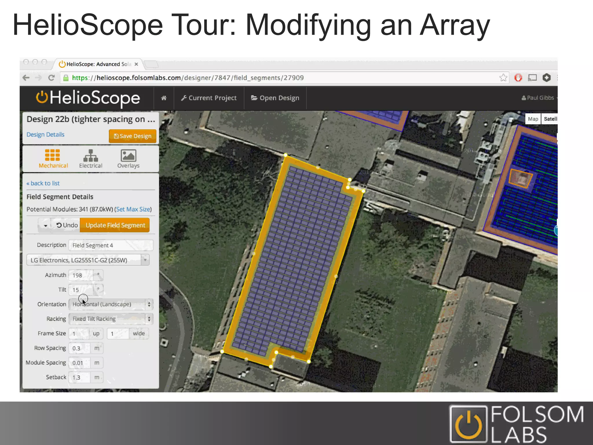
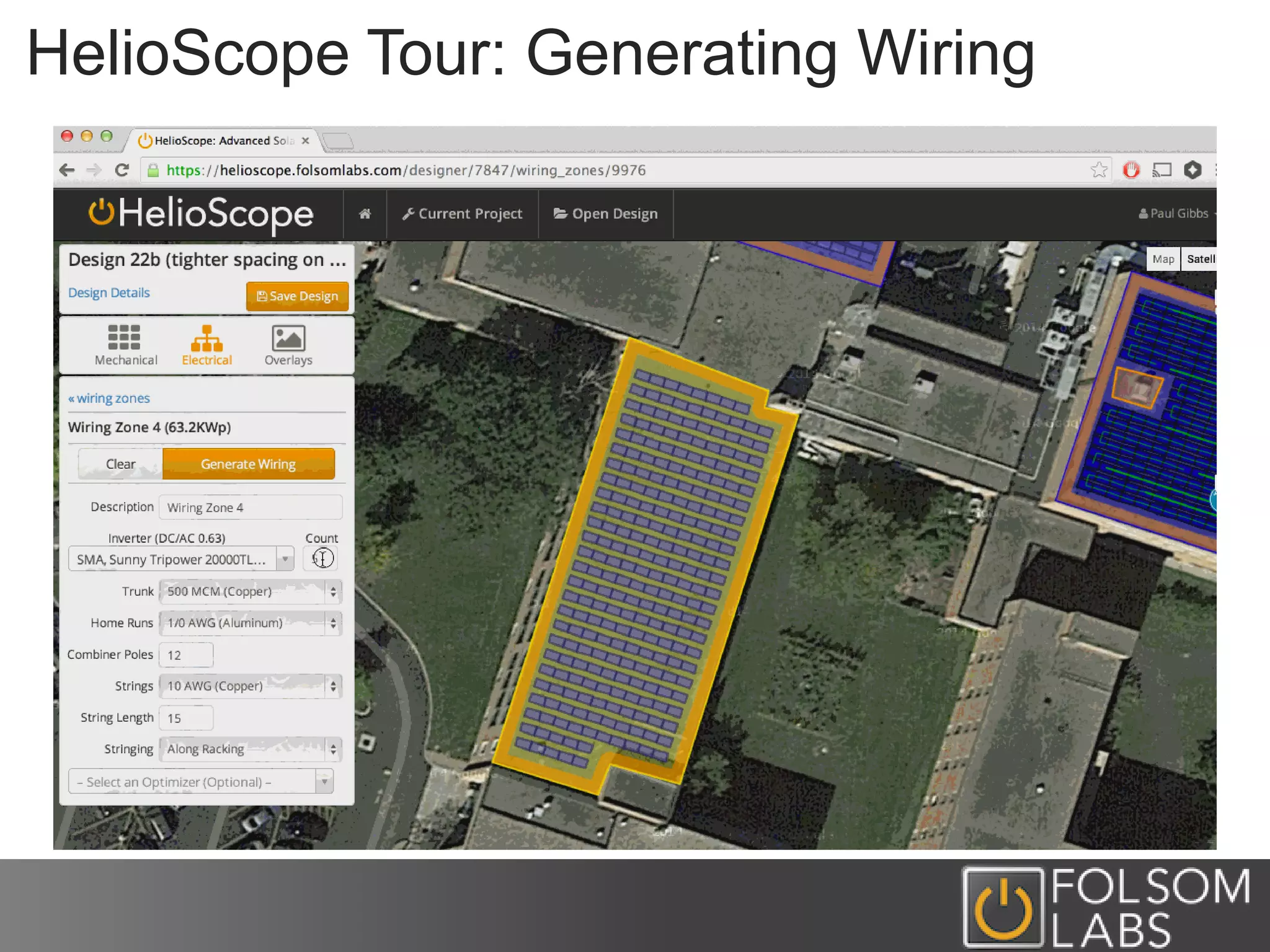
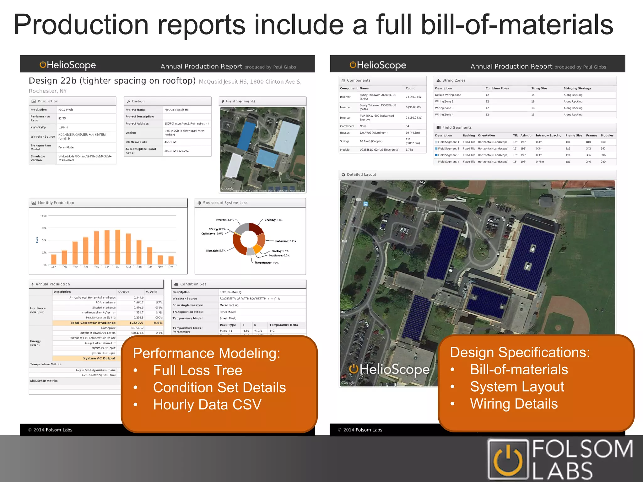
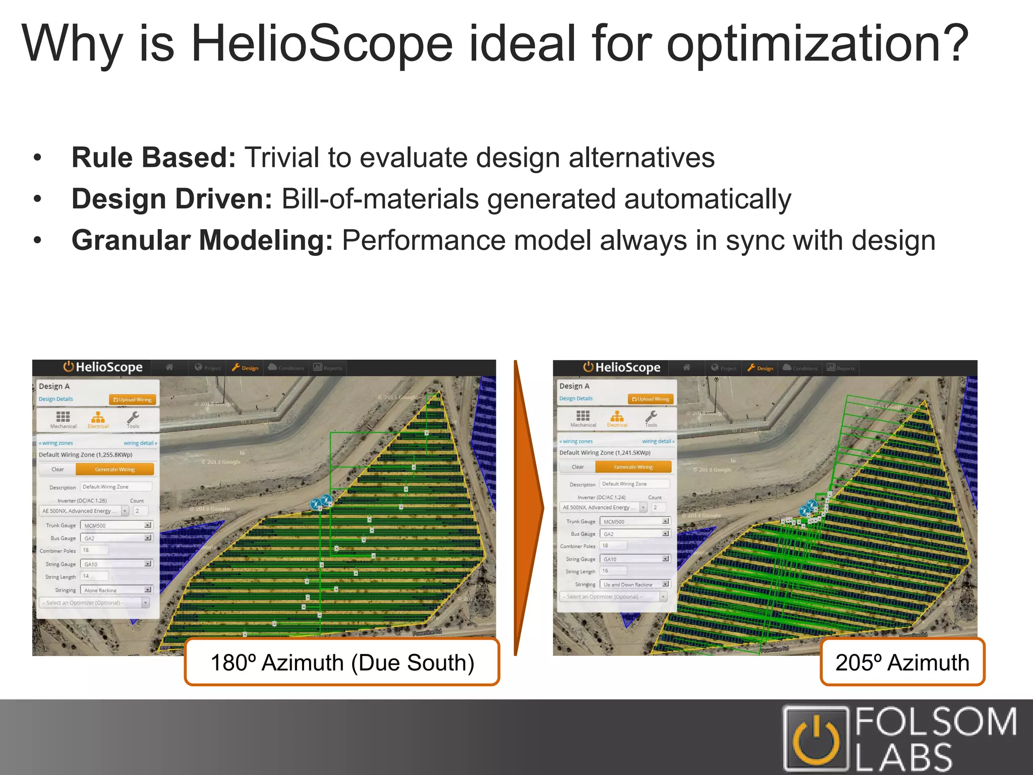
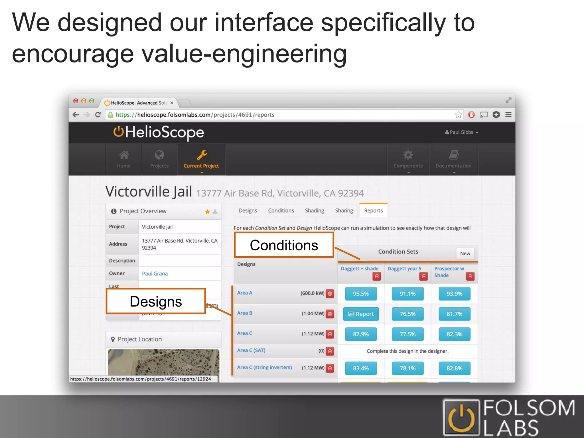
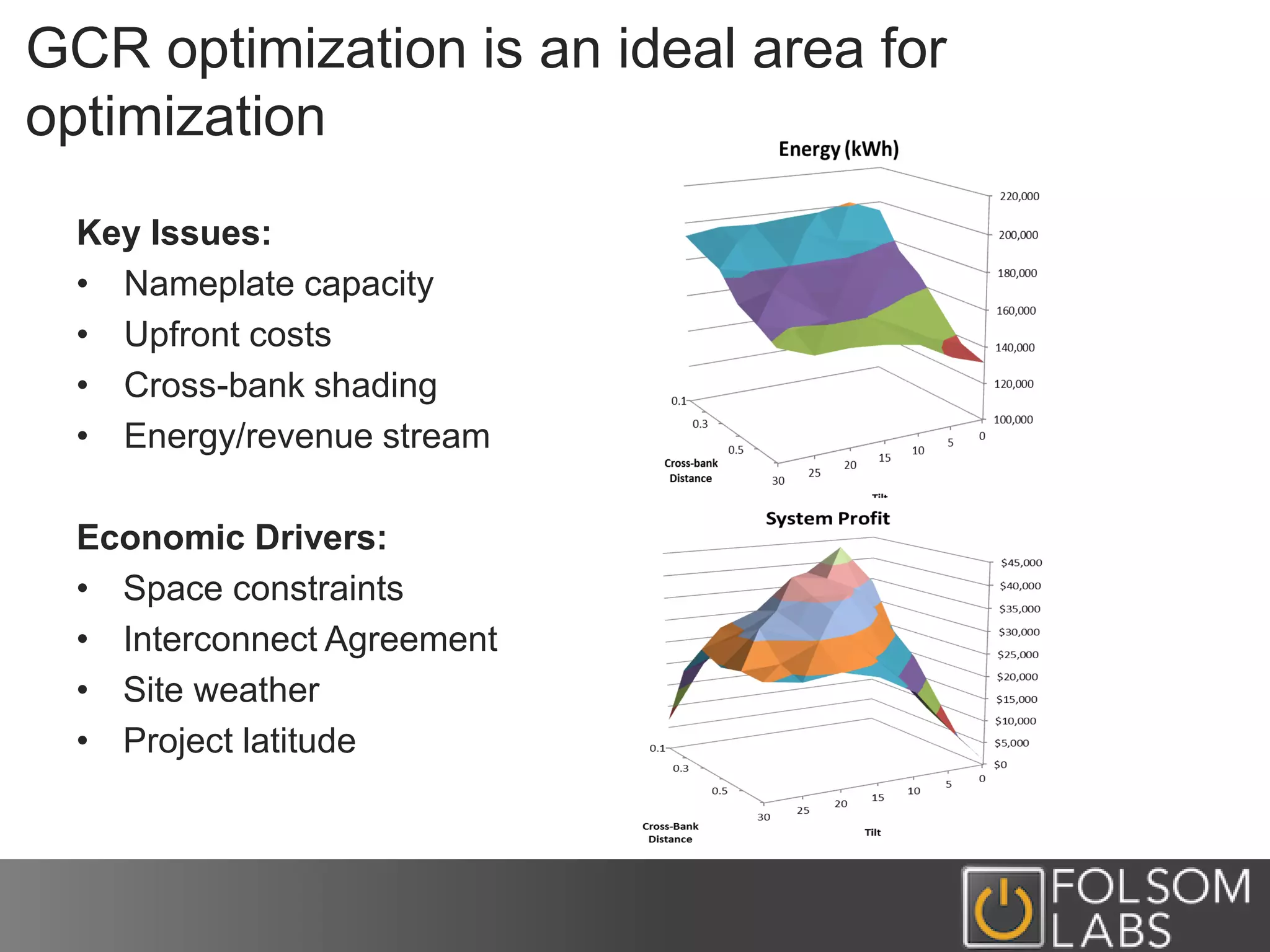
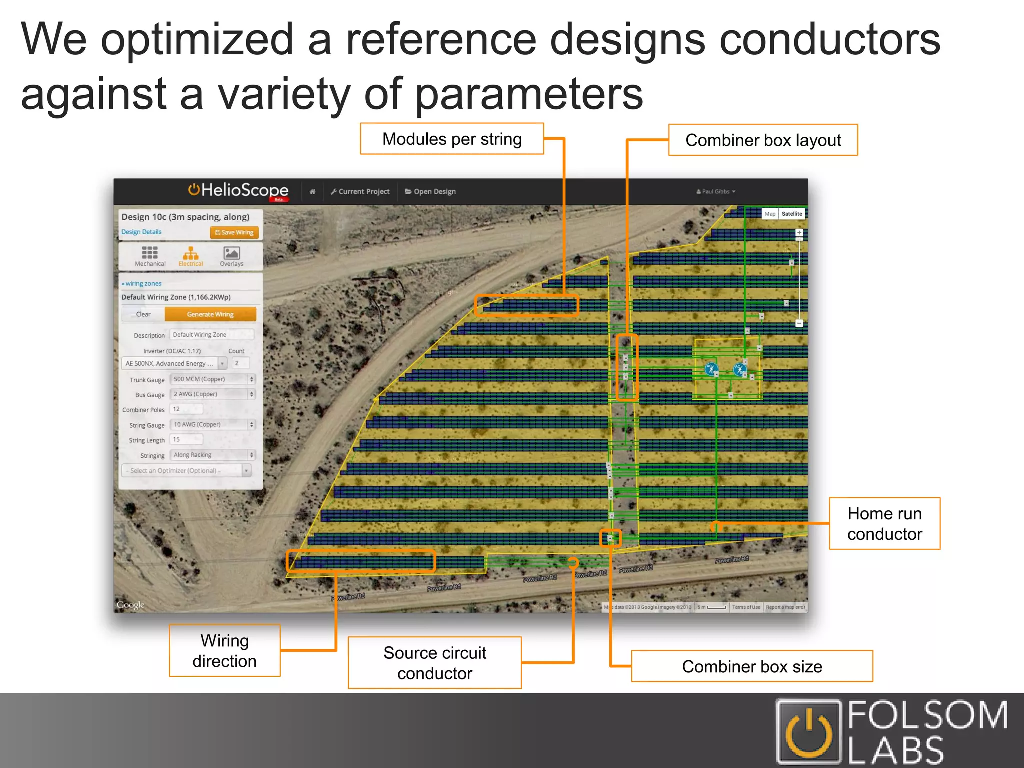
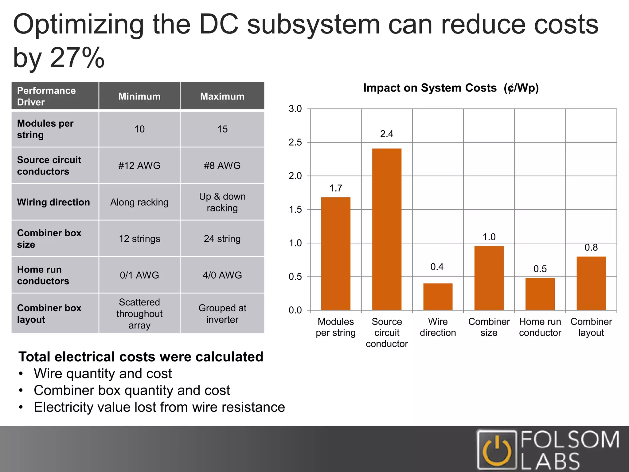
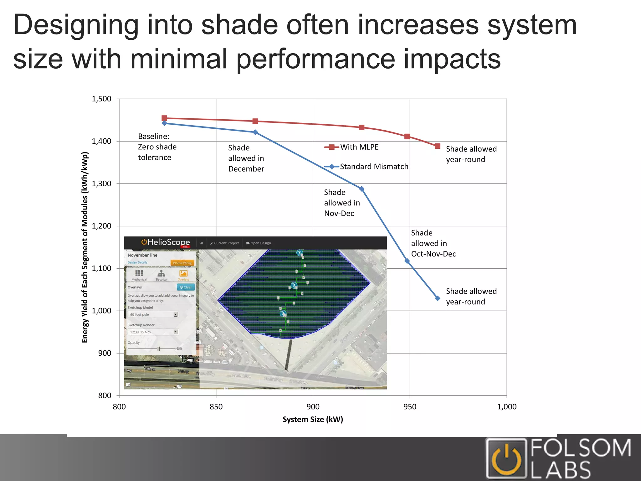
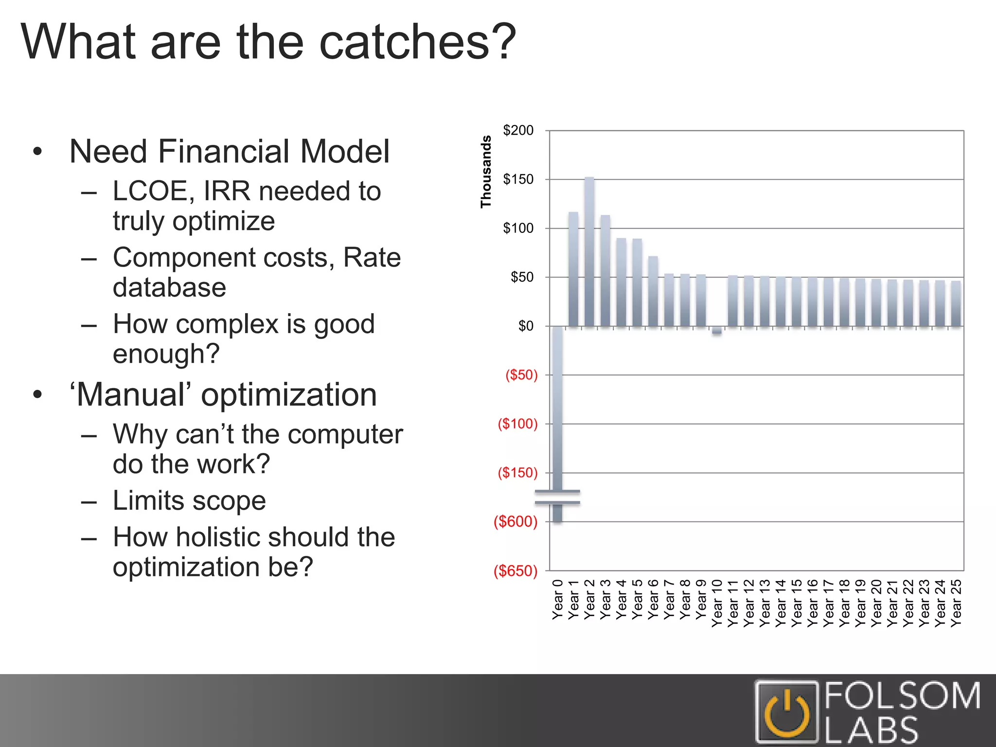
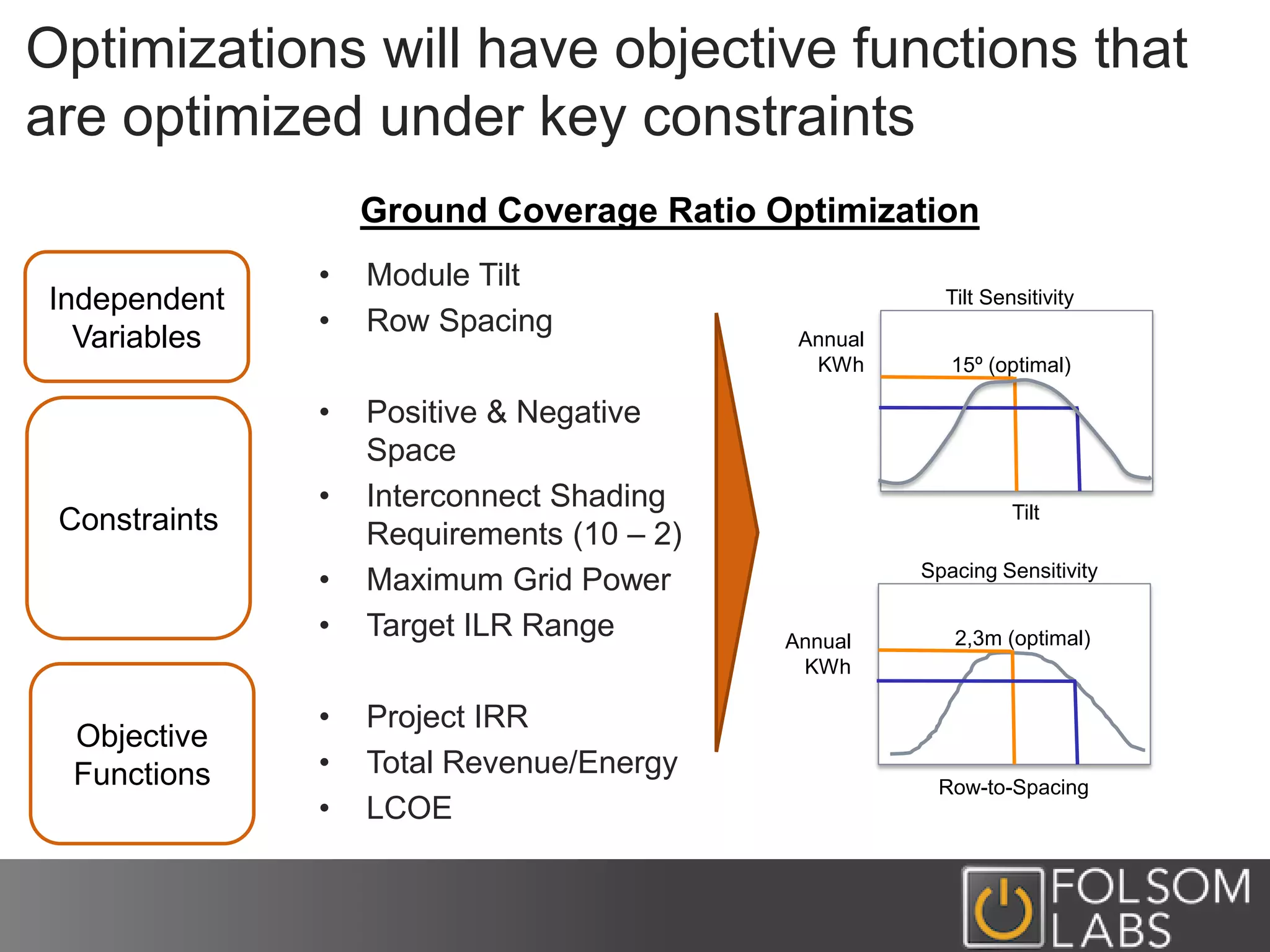
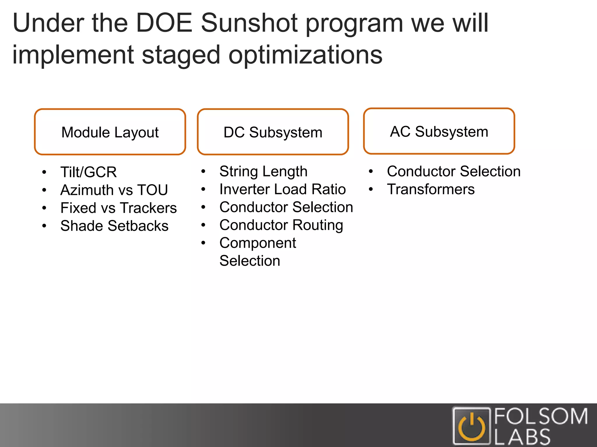
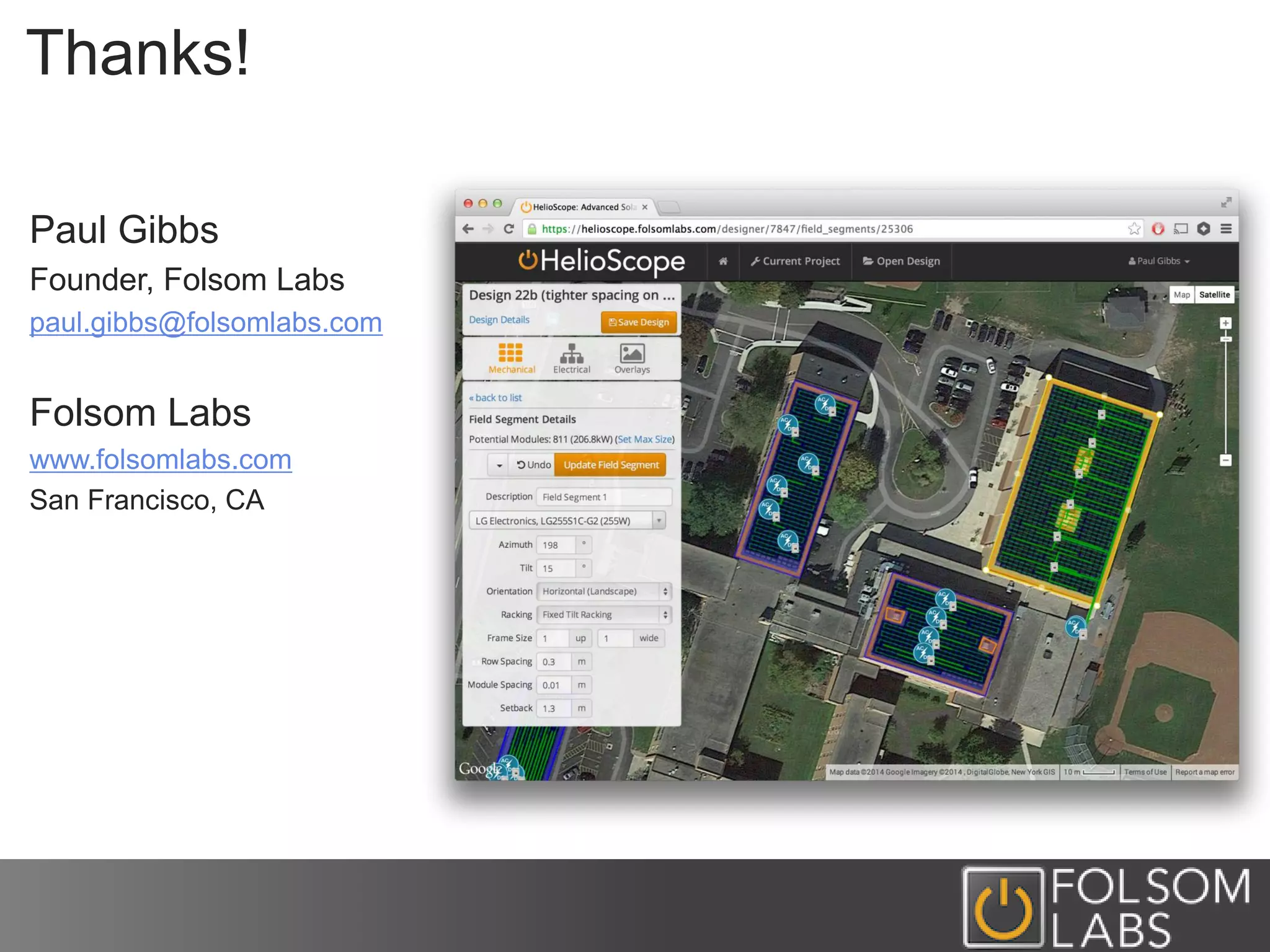
Optimizing PV Designs with HelioScope
Sandia Performance Modeling Workshop
Paul Gibbs
May 5, 2014
paul.gibbs@folsomlabs.com
Agenda
• What is HelioScope and why is it good for
optimization?
• Case Studies in PV System Optimization
– Ground Coverage Ratio
– DC Plant Design
– Designing into Shade
• Looking forward: automating optimization
HelioScope is a design-driven PV modeling tool
Principles
• Design-driven
• Component-level
• Cloud-based
Values
• Throughput Velocity
• Value Engineering
HelioScope Tour: Adding a Field Segment
HelioScope Tour: Modifying an Array
HelioScope Tour: Generating Wiring
Production reports include a full bill-of-materials
Performance Modeling:
• Full Loss Tree
• Condition Set Details
• Hourly Data CSV
Design Specifications:
• Bill-of-materials
• System Layout
• Wiring Details
Why is HelioScope ideal for optimization?
• Rule Based: Trivial to evaluate design alternatives
• Design Driven: Bill-of-materials generated automatically
• Granular Modeling: Performance model always in sync with design
180º Azimuth (Due South) 205º Azimuth
We designed our interface specifically to
encourage value-engineering
Designs
Conditions
GCR optimization is an ideal area for
optimization
Key Issues:
• Nameplate capacity
• Upfront costs
• Cross-bank shading
• Energy/revenue stream
Economic Drivers:
• Space constraints
• Interconnect Agreement
• Site weather
• Project latitude
We optimized a reference designs conductors
against a variety of parameters
Modules per string
Combiner box size
Source circuit
conductor
Combiner box layout
Wiring
direction
Home run
conductor
Optimizing the DC subsystem can reduce costs
by 27%
Total electrical costs were calculated
• Wire quantity and cost
• Combiner box quantity and cost
• Electricity value lost from wire resistance
Performance
Driver
Minimum Maximum
Modules per
string
10 15
Source circuit
conductors
#12 AWG #8 AWG
Wiring direction Along racking
Up & down
racking
Combiner box
size
12 strings 24 string
Home run
conductors
0/1 AWG 4/0 AWG
Combiner box
layout
Scattered
throughout
array
Grouped at
inverter
1.7
2.4
0.4
1.0
0.5
0.8
0.0
0.5
1.0
1.5
2.0
2.5
3.0
Modules
per string
Source
circuit
conductor
Wire
direction
Combiner
size
Home run
conductor
Combiner
layout
Impact on System Costs (¢/Wp)
Designing into shade often increases system
size with minimal performance impacts
800
900
1,000
1,100
1,200
1,300
1,400
1,500
800 850 900 950 1,000
EnergyYieldofEachSegmentofModules(kWh/kWp)
System Size (kW)
With MLPE
Standard Mismatch
Baseline:
Zero shade
tolerance
Shade
allowed in
December
Shade
allowed in
Nov-Dec
Shade
allowed in
Oct-Nov-Dec
Shade allowed
year-round
Shade allowed
year-round
($250)
($200)
($150)
($100)
($50)
$0
$50
$100
$150
$200
Year0
Year1
Year2
Year3
Year4
Year5
Year6
Year7
Year8
Year9
Year10
Year11
Year12
Year13
Year14
Year15
Year16
Year17
Year18
Year19
Year20
Year21
Year22
Year23
Year24
Year25
Thousands
What are the catches?
• Need Financial Model
– LCOE, IRR needed to
truly optimize
– Component costs, Rate
database
– How complex is good
enough?
• ‘Manual’ optimization
– Why can’t the computer
do the work?
– Limits scope
– How holistic should the
optimization be? ($650)
($600)
DOE Sunshot Award to extend HelioScope with
Design Optimization features
• Started 1Q2014
• Augments HelioScope with optimization features
– Automated optimization
– Financial modelCustomer feedback: staged
optimizations are ideal
– At start of project, goal is maximize energy or revenue
– As project progresses, several deep dives (e.g. wiring)
Optimizations will have objective functions that
are optimized under key constraints
• Module Tilt
• Row Spacing
• Positive & Negative
Space
• Interconnect Shading
Requirements (10 – 2)
• Maximum Grid Power
• Target ILR Range
• Project IRR
• Total Revenue/Energy
• LCOE
Independent
Variables
Constraints
Objective
Functions
Ground Coverage Ratio Optimization
Tilt
Annual
KWh
Tilt Sensitivity
15º (optimal)
Annual
KWh
Spacing Sensitivity
2,3m (optimal)
Row-to-Spacing
Under the DOE Sunshot program we will
implement staged optimizations
Module Layout DC Subsystem AC Subsystem
• Tilt/GCR
• Azimuth vs TOU
• Fixed vs Trackers
• Shade Setbacks
• String Length
• Inverter Load Ratio
• Conductor Selection
• Conductor Routing
• Component
Selection
• Conductor Selection
• Transformers
Thanks!
Paul Gibbs
Founder, Folsom Labs
paul.gibbs@folsomlabs.com
Folsom Labs
www.folsomlabs.com
San Francisco, CA

2014 PV Performance Modeling Workshop: Optimizing PV Designs with HelioScope: Paul Gibbs, Folsom Labs

  • 1.
    Optimizing PV Designswith HelioScope Sandia Performance Modeling Workshop Paul Gibbs May 5, 2014 paul.gibbs@folsomlabs.com
  • 2.
    Agenda • What isHelioScope and why is it good for optimization? • Case Studies in PV System Optimization – Ground Coverage Ratio – DC Plant Design – Designing into Shade • Looking forward: automating optimization
  • 3.
    HelioScope is adesign-driven PV modeling tool Principles • Design-driven • Component-level • Cloud-based Values • Throughput Velocity • Value Engineering
  • 4.
    HelioScope Tour: Addinga Field Segment
  • 5.
  • 6.
  • 7.
    Production reports includea full bill-of-materials Performance Modeling: • Full Loss Tree • Condition Set Details • Hourly Data CSV Design Specifications: • Bill-of-materials • System Layout • Wiring Details
  • 8.
    Why is HelioScopeideal for optimization? • Rule Based: Trivial to evaluate design alternatives • Design Driven: Bill-of-materials generated automatically • Granular Modeling: Performance model always in sync with design 180º Azimuth (Due South) 205º Azimuth
  • 9.
    We designed ourinterface specifically to encourage value-engineering Designs Conditions
  • 10.
    GCR optimization isan ideal area for optimization Key Issues: • Nameplate capacity • Upfront costs • Cross-bank shading • Energy/revenue stream Economic Drivers: • Space constraints • Interconnect Agreement • Site weather • Project latitude
  • 11.
    We optimized areference designs conductors against a variety of parameters Modules per string Combiner box size Source circuit conductor Combiner box layout Wiring direction Home run conductor
  • 12.
    Optimizing the DCsubsystem can reduce costs by 27% Total electrical costs were calculated • Wire quantity and cost • Combiner box quantity and cost • Electricity value lost from wire resistance Performance Driver Minimum Maximum Modules per string 10 15 Source circuit conductors #12 AWG #8 AWG Wiring direction Along racking Up & down racking Combiner box size 12 strings 24 string Home run conductors 0/1 AWG 4/0 AWG Combiner box layout Scattered throughout array Grouped at inverter 1.7 2.4 0.4 1.0 0.5 0.8 0.0 0.5 1.0 1.5 2.0 2.5 3.0 Modules per string Source circuit conductor Wire direction Combiner size Home run conductor Combiner layout Impact on System Costs (¢/Wp)
  • 13.
    Designing into shadeoften increases system size with minimal performance impacts 800 900 1,000 1,100 1,200 1,300 1,400 1,500 800 850 900 950 1,000 EnergyYieldofEachSegmentofModules(kWh/kWp) System Size (kW) With MLPE Standard Mismatch Baseline: Zero shade tolerance Shade allowed in December Shade allowed in Nov-Dec Shade allowed in Oct-Nov-Dec Shade allowed year-round Shade allowed year-round
  • 14.
    ($250) ($200) ($150) ($100) ($50) $0 $50 $100 $150 $200 Year0 Year1 Year2 Year3 Year4 Year5 Year6 Year7 Year8 Year9 Year10 Year11 Year12 Year13 Year14 Year15 Year16 Year17 Year18 Year19 Year20 Year21 Year22 Year23 Year24 Year25 Thousands What are thecatches? • Need Financial Model – LCOE, IRR needed to truly optimize – Component costs, Rate database – How complex is good enough? • ‘Manual’ optimization – Why can’t the computer do the work? – Limits scope – How holistic should the optimization be? ($650) ($600)
  • 15.
    DOE Sunshot Awardto extend HelioScope with Design Optimization features • Started 1Q2014 • Augments HelioScope with optimization features – Automated optimization – Financial modelCustomer feedback: staged optimizations are ideal – At start of project, goal is maximize energy or revenue – As project progresses, several deep dives (e.g. wiring)
  • 16.
    Optimizations will haveobjective functions that are optimized under key constraints • Module Tilt • Row Spacing • Positive & Negative Space • Interconnect Shading Requirements (10 – 2) • Maximum Grid Power • Target ILR Range • Project IRR • Total Revenue/Energy • LCOE Independent Variables Constraints Objective Functions Ground Coverage Ratio Optimization Tilt Annual KWh Tilt Sensitivity 15º (optimal) Annual KWh Spacing Sensitivity 2,3m (optimal) Row-to-Spacing
  • 17.
    Under the DOESunshot program we will implement staged optimizations Module Layout DC Subsystem AC Subsystem • Tilt/GCR • Azimuth vs TOU • Fixed vs Trackers • Shade Setbacks • String Length • Inverter Load Ratio • Conductor Selection • Conductor Routing • Component Selection • Conductor Selection • Transformers
  • 18.
    Thanks! Paul Gibbs Founder, FolsomLabs paul.gibbs@folsomlabs.com Folsom Labs www.folsomlabs.com San Francisco, CA