In a perfectly competitive market:
- Many buyers and sellers exist
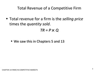
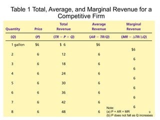
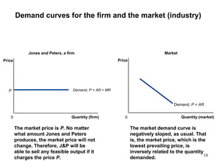
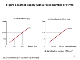
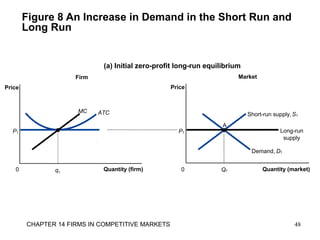
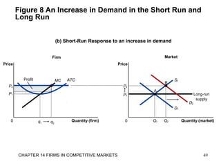
- Firms are price takers and the actions of any single firm do not impact the market price
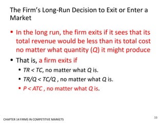
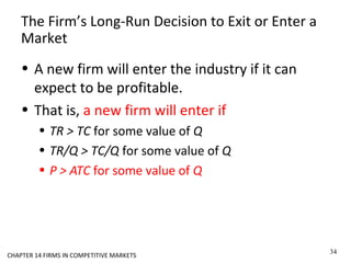
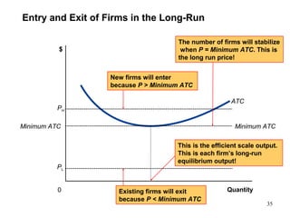
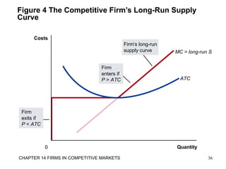
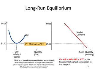
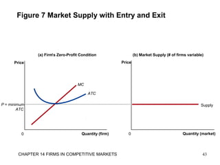
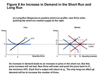
- In the long run, firms will enter or exit the market until price equals minimum average total cost and economic profit is zero.
Mankiew chapter 7 Consumers, Producers, and the Efficiency of MarketsAbd ELRahman ALFar
What is consumer surplus? How is it related to the demand curve?
What is producer surplus? How is it related to the supply curve?
Do markets produce a desirable allocation of resources? Or could the market outcome be improved upon?
This short revision video provides an overview of three forms of imperfect competition, namely monopoly, oligopoly and imperfect competition. It considers too the likely impact of each market structure on allocative, productive and dynamic efficiency.
This presentation basically tells how the firm makes decisions in a competitive market. To make concepts here more understable, I have prepared graphs and mathematical equations.
perfect competition, monopoly, monopolistic and oligopolysandypkapoor
Price determination under different market structure and characterstics of all these market stractures along with graphical presentation of Perfect competition, Monopoly, Monopolistic and Oligopoly market structue
Synthetic Fiber Construction in lab .pptxPavel ( NSTU)
Synthetic fiber production is a fascinating and complex field that blends chemistry, engineering, and environmental science. By understanding these aspects, students can gain a comprehensive view of synthetic fiber production, its impact on society and the environment, and the potential for future innovations. Synthetic fibers play a crucial role in modern society, impacting various aspects of daily life, industry, and the environment. ynthetic fibers are integral to modern life, offering a range of benefits from cost-effectiveness and versatility to innovative applications and performance characteristics. While they pose environmental challenges, ongoing research and development aim to create more sustainable and eco-friendly alternatives. Understanding the importance of synthetic fibers helps in appreciating their role in the economy, industry, and daily life, while also emphasizing the need for sustainable practices and innovation.
The Roman Empire A Historical Colossus.pdfkaushalkr1407
The Roman Empire, a vast and enduring power, stands as one of history's most remarkable civilizations, leaving an indelible imprint on the world. It emerged from the Roman Republic, transitioning into an imperial powerhouse under the leadership of Augustus Caesar in 27 BCE. This transformation marked the beginning of an era defined by unprecedented territorial expansion, architectural marvels, and profound cultural influence.
The empire's roots lie in the city of Rome, founded, according to legend, by Romulus in 753 BCE. Over centuries, Rome evolved from a small settlement to a formidable republic, characterized by a complex political system with elected officials and checks on power. However, internal strife, class conflicts, and military ambitions paved the way for the end of the Republic. Julius Caesar’s dictatorship and subsequent assassination in 44 BCE created a power vacuum, leading to a civil war. Octavian, later Augustus, emerged victorious, heralding the Roman Empire’s birth.
Under Augustus, the empire experienced the Pax Romana, a 200-year period of relative peace and stability. Augustus reformed the military, established efficient administrative systems, and initiated grand construction projects. The empire's borders expanded, encompassing territories from Britain to Egypt and from Spain to the Euphrates. Roman legions, renowned for their discipline and engineering prowess, secured and maintained these vast territories, building roads, fortifications, and cities that facilitated control and integration.
The Roman Empire’s society was hierarchical, with a rigid class system. At the top were the patricians, wealthy elites who held significant political power. Below them were the plebeians, free citizens with limited political influence, and the vast numbers of slaves who formed the backbone of the economy. The family unit was central, governed by the paterfamilias, the male head who held absolute authority.
Culturally, the Romans were eclectic, absorbing and adapting elements from the civilizations they encountered, particularly the Greeks. Roman art, literature, and philosophy reflected this synthesis, creating a rich cultural tapestry. Latin, the Roman language, became the lingua franca of the Western world, influencing numerous modern languages.
Roman architecture and engineering achievements were monumental. They perfected the arch, vault, and dome, constructing enduring structures like the Colosseum, Pantheon, and aqueducts. These engineering marvels not only showcased Roman ingenuity but also served practical purposes, from public entertainment to water supply.
The French Revolution, which began in 1789, was a period of radical social and political upheaval in France. It marked the decline of absolute monarchies, the rise of secular and democratic republics, and the eventual rise of Napoleon Bonaparte. This revolutionary period is crucial in understanding the transition from feudalism to modernity in Europe.
For more information, visit-www.vavaclasses.com
Biological screening of herbal drugs: Introduction and Need for
Phyto-Pharmacological Screening, New Strategies for evaluating
Natural Products, In vitro evaluation techniques for Antioxidants, Antimicrobial and Anticancer drugs. In vivo evaluation techniques
for Anti-inflammatory, Antiulcer, Anticancer, Wound healing, Antidiabetic, Hepatoprotective, Cardio protective, Diuretics and
Antifertility, Toxicity studies as per OECD guidelines
Embracing GenAI - A Strategic ImperativePeter Windle
Artificial Intelligence (AI) technologies such as Generative AI, Image Generators and Large Language Models have had a dramatic impact on teaching, learning and assessment over the past 18 months. The most immediate threat AI posed was to Academic Integrity with Higher Education Institutes (HEIs) focusing their efforts on combating the use of GenAI in assessment. Guidelines were developed for staff and students, policies put in place too. Innovative educators have forged paths in the use of Generative AI for teaching, learning and assessments leading to pockets of transformation springing up across HEIs, often with little or no top-down guidance, support or direction.
This Gasta posits a strategic approach to integrating AI into HEIs to prepare staff, students and the curriculum for an evolving world and workplace. We will highlight the advantages of working with these technologies beyond the realm of teaching, learning and assessment by considering prompt engineering skills, industry impact, curriculum changes, and the need for staff upskilling. In contrast, not engaging strategically with Generative AI poses risks, including falling behind peers, missed opportunities and failing to ensure our graduates remain employable. The rapid evolution of AI technologies necessitates a proactive and strategic approach if we are to remain relevant.
Francesca Gottschalk - How can education support child empowerment.pptxEduSkills OECD
Francesca Gottschalk from the OECD’s Centre for Educational Research and Innovation presents at the Ask an Expert Webinar: How can education support child empowerment?
Unit 8 - Information and Communication Technology (Paper I).pdfThiyagu K
This slides describes the basic concepts of ICT, basics of Email, Emerging Technology and Digital Initiatives in Education. This presentations aligns with the UGC Paper I syllabus.
Palestine last event orientationfvgnh .pptxRaedMohamed3
An EFL lesson about the current events in Palestine. It is intended to be for intermediate students who wish to increase their listening skills through a short lesson in power point.
2. WHAT IS A COMPETITIVE MARKET?
• In a perfectly competitive market
• There are many buyers
• There are many sellers
• Firms can freely enter or exit the market, in the long run.
• In the short run, the number of firms is assumed fixed
(constant).
• All sellers sell the same product.
2
CHAPTER 14 FIRMS IN COMPETITIVE MARKETS
3. WHAT IS A COMPETITIVE MARKET?
• As a result:
• The actions of any single buyer or seller have a
negligible impact on the market price.
• That is, the market price is unaffected by the amount
bought by a buyer or the amount sold by a seller
• Therefore, every buyer and every seller takes the
market price as given.
• Everybody is a ‘price taker’
3
CHAPTER 14 FIRMS IN COMPETITIVE MARKETS
4. Price takers
• A firm in a perfectly competitive market cannot stay in
business if its price is higher than what the other firms are
charging
• No firm would be able to raise the market price by reducing
production and attempting to create a shortage.
• Conversely, there is no danger that a firm would drive the
market price down by producing too much.
• Therefore, no firm would want to charge a price lower than
what the others are charging.
• In short, each firm takes the prevailing market price as a given
—like the weather—and charges that price.
4
CHAPTER 14 FIRMS IN COMPETITIVE MARKETS
5. Total Revenue of a Competitive Firm
• Total revenue for a firm is the selling price
times the quantity sold.
TR = PTR = P ×× QQ
• We saw this in Chapters 5 and 13We saw this in Chapters 5 and 13
5
CHAPTER 14 FIRMS IN COMPETITIVE MARKETS
6. Average Revenue of a Competitive Firm
• Average revenue is the revenue per unit sold
• P = AR.
• This is simply because all units sold are sold at the
same price.
A v e r a g e R e v e n u e =
T o t a l r e v e n u e
Q u a n t i t y
P r i c e Q u a n t i t y
Q u a n t i t y
P r i c e
=
×
=
6
7. Marginal Revenue of a Competitive Firm
• Marginal Revenue is the increase (Δ) in total
revenue when an additional unit is sold.
MRMR == ∆∆TRTR // ∆∆QQ
7
CHAPTER 14 FIRMS IN COMPETITIVE MARKETS
8. The Revenue of a Competitive Firm
• In perfect competition, marginal revenue
equals price: P = MR.
• We saw earlier that P = AR
• Therefore, for all firms in perfect competition,
P = AR = MR
8
CHAPTER 14 FIRMS IN COMPETITIVE MARKETS
9. Table 1 Total, Average, and Marginal Revenue for a
Competitive Firm
Note:
(a) P = AR = MR
(b) P does not fall as Q increases
9
10. Demand curves for the firm and the market (industry)
Jones and Peters, a firm
Quantity (firm)0
Price
Market
Quantity (market)
Price
0
Demand, P = AR
P
The market demand curve is
negatively sloped, as usual. That
is, the market price, which is the
lowest prevailing price, is
inversely related to the quantity
demanded.
The market price is P. No matter
what amount Jones and Peters
produces, the market price will not
change. Therefore, J&P will be
able to sell any feasible output if it
charges the price P.
Demand, P = AR = MR
10
11. Supply
• We have just seen the
demand curves for a
firm and for the
entire industry
• Next, we need to
work out what the
supply curves look
like
CHAPTER 14 FIRMS IN COMPETITIVE MARKETS
11
12. Supply: short run and long run
• The analysis of supply in perfect competition
depends on whether it is the short run or the
long run.
12
CHAPTER 14 FIRMS IN COMPETITIVE MARKETS
13. Short run and long run: assumptions
• The quantity of a resource used by a firm may
be fixed in the short run but not in the long
run.
• Example: If a firm currently has three custom-made
machines and if it takes six months to get new machines,
then the firm is stuck with its three machines for the next
six months.
• All fixed costs are sunk costs in the short run
but not in the long run
• The number of firms in an industry is fixed in
the short run but not in the long run
13
CHAPTER 14 FIRMS IN COMPETITIVE MARKETS
15. Shut Down and Exit
• Before a firm decides how much to supply, it
must decide whether or not to stay in business
• A shutdown refers to a short-run decision to
stop production temporarily, perhaps because
of poor market conditions.
• Exit refers to a long-run decision to end
production permanently.
15
CHAPTER 14 FIRMS IN COMPETITIVE MARKETS
16. The Firm’s Short-Run Decision to Shut Down
• A firm will shut down (temporarily) if its
variable costs exceed its total revenue, no
matter what quantity it produces
• Its fixed costs do not matter!
• This is because
• Fixed costs are sunk costs in the short run
• sunk costs are defined as costs that will have to be paid
even if the firm shuts down.
• Therefore, FC cannot affect a firm’s decision on
whether to stay open or shut down
16
CHAPTER 14 FIRMS IN COMPETITIVE MARKETS
17. Sunk Costs
• Sunk costs will have to be paid even when a
firm is in a temporary shutdown.
• Examples:
• If the firm signs a long-term contract with its landlord,
the rent will have to be paid even when the firm is
temporarily shut down.
• Some maintenance costs will have to be incurred even
when the firm is shut down.
• The firm may be under contract to provide customer
service to past customers even after it shuts down.
17
CHAPTER 14 FIRMS IN COMPETITIVE MARKETS
18. The Firm’s Short-Run Decision to Shut Down
• Total Revenue = $1000 per month
• Variable Cost = $800 per month
• Fixed Cost = $400 per month
• Profit = –$200 per month (a loss)
• Q: Should this firm stay in business or should it shut down
for the time being?
• A: It should stay in business
• If it shuts down, the fixed cost (say, rent owed to the landlord) will
still have to be paid—because it is sunk!—and the loss will then be
even higher, $400 per month.
18
CHAPTER 14 FIRMS IN COMPETITIVE MARKETS
19. The Firm’s Short-Run Decision to Shut Down
• Total Revenue = $1000 per month
• Variable Cost = $1200 per month
• Fixed Cost = $400 per month
• Profit = –$600 per month (a loss)
• Q: Should this firm stay in business or should it shut
down for the time being?
• A: It should shut down.
• The lesson from this and the previous slide is
that …
19
CHAPTER 14 FIRMS IN COMPETITIVE MARKETS
20. The Firm’s Short-Run Decision to Shut Down
• A firm shuts down if total revenue is less than
variable cost, no matter what quantity the firm
produces. That is,
• A firm shuts down if
• TR < VC, no matter what Q is, or
• TR/Q < VC/Q, no matter what Q is, or
• P < AVC, no matter what Q is.
20
CHAPTER 14 FIRMS IN COMPETITIVE MARKETS
21. A Firm’s Shut Down Decision
Quantity
AVC
0
$
The firm shuts down
because P < Minimum AVC
The firm stays open
because P > Minimum AVC
Minimum AVC Minimum AVC
PH
PL
21
22. Table 2 Profit Maximization: A Numerical Example
Is it possible
to figure out
the profit-
maximizing
output from
just the MR
and MC
numbers?
Yes, it is where
MR = MC.
22
23. Figure 1 Profit Maximization for a Competitive Firm
Quantity0
Costs
and
Revenue
MC
ATC
AVC
MC1
Q1
MC2
Q2
The firm maximizes
profit by producing
the quantity at which
marginal cost equals
marginal revenue.
QMAX
P = MR1 = MR2 P = AR = MR
23CHAPTER 14
Therefore, P = AR =
MR = MC is the
fingerprint of perfect
competition
We have seen before
that, as firms are price
takers in perfect
competition, P = AR =
MR.
We have also seen
that, profit
maximization implies
MR = MC.
24. PROFIT MAXIMIZATION AND THE COMPETITIVE
FIRM’S SUPPLY CURVE
• Profit maximization occurs at the quantity
where marginal revenue equals marginal cost.
• This is a crucial principle in understanding the
behavior of firms
24
CHAPTER 14 FIRMS IN COMPETITIVE MARKETS
25. PROFIT MAXIMIZATION AND THE COMPETITIVE
FIRM’S SUPPLY CURVE
• When MR > MC increase Q
• When MR < MC decrease Q
• WhenWhen MR = MCMR = MC Profit is maximized;Profit is maximized;
stick with thisstick with this Q.Q.
25
CHAPTER 14 FIRMS IN COMPETITIVE MARKETS
27. Figure 2 Marginal Cost as the Competitive Firm’s
Supply Curve
Quantity0
Price
MC
ATC
AVC
P1
Q1
P2
Q2
This section of the
firm’s MC curve is
also the firm’s supply
curve.
27
28. Figure 3 The Competitive Firm’s Short Run Supply
Curve
MC
Quantity
ATC
AVC
0
Costs
Firm
shuts
down if
P<AVC
Firm’s short-run
supply curve
If P > AVC, firm will
continue to produce
in the short run.
If P > ATC, the firm
will continue to
produce at a profit.
28CHAPTER 14 FIRMS IN COMPETITIVE MARKETS
What can shift the supply
curve to the right?
29. The Short Run: Market Supply with a Fixed
Number of Firms
• The market supply curve is the horizontal sum
of the individual firms’ short run supply curves.
29
CHAPTER 14 FIRMS IN COMPETITIVE MARKETS
30. Figure 6 Market Supply with a Fixed Number of Firms
(a) Individual Firm Supply
Quantity (firm)0
Price
MC
1.00
100
$2.00
200
(b) Market Supply (# of firms fixed)
Quantity (market)0
Price
Supply
1.00
100,000
$2.00
200,000
Q: What is the number of firms?
30
CHAPTER 14 FIRMS IN COMPETITIVE MARKETS
31. Short-Run Equilibrium: back where we began!
(a) Individual Firm Supply
Quantity (firm)0
Price
MC
1.00
100
$2.00
200
(b) Market Supply (# of firms fixed)
Quantity (market)0
Price
Supply
1.00
100,000
$2.00
200,000
31CHAPTER 14 FIRMS IN COMPETITIVE MARKETS
DemandL
DemandH
32. THE LONG RUN
Price = Minimum ATC; profit = zero; demand has no effect on price, and
no effect on the quantity produced by a firm; demand does affect the
quantity produced by the industry, and the number of firms in the
industry
32
33. The Firm’s Long-Run Decision to Exit or Enter a
Market
• In the long run, the firm exits if it sees that its
total revenue would be less than its total cost
no matter what quantity (Q) it might produce
• That is, a firm exits if
• TR < TC, no matter what Q is.
• TR/Q < TC/Q , no matter what Q is.
• P < ATC , no matter what Q is.
33
CHAPTER 14 FIRMS IN COMPETITIVE MARKETS
34. The Firm’s Long-Run Decision to Exit or Enter a
Market
• A new firm will enter the industry if it can
expect to be profitable.
• That is, a new firm will enter if
• TR > TC for some value of Q
• TR/Q > TC/Q for some value of Q
• P > ATC for some value of Q
34
CHAPTER 14 FIRMS IN COMPETITIVE MARKETS
35. Entry and Exit of Firms in the Long-Run
Quantity
ATC
0
$
Minimum ATC Minimum ATC
Existing firms will exit
because P < Minimum ATC
The number of firms will stabilize
when P = Minimum ATC. This is
the long run price!
New firms will enter
because P > Minimum ATC
PH
PL
35
This is the efficient scale output.
This is each firm’s long-run
equilibrium output!
36. Figure 4 The Competitive Firm’s Long-Run Supply
Curve
MC = long-run S
Firm
exits if
P < ATC
Quantity
ATC
0
Costs
Firm’s long-run
supply curve
Firm
enters if
P > ATC
36CHAPTER 14 FIRMS IN COMPETITIVE MARKETS
37. ATC
THE SUPPLY CURVE IN A COMPETITIVE
MARKET
• A Firm’s Short-Run Supply
Curve
• The portion of its (short run)
marginal cost curve that lies
above the (short run) average
variable cost curve.
• A Firm’s Long-Run Supply
Curve
• The portion of its (long run)
marginal cost curve that lies
above the (long run) average
total cost curve.
37
CHAPTER 14 FIRMS IN COMPETITIVE MARKETS
MC
ATC
AVC
38. Long-Run Equilibrium
This is it, as far as long-run equilibrium is concerned!
How many firms are there in long-run equilibrium?
What would happen if demand moves left (decreases)?
What could cause prices to increase? 38
ATC
PricePrice
Quantity
(industry)
Quantity
(firm)
6,000200
(efficient
scale)
$1.50$1.50 P = Minimum ATC =
Market
Demand
P = AR = MR = MC = ATC is the
fingerprint of perfect competition in
the long run.
39. A Firm’s Profit
• Profit equals total revenue minus total costs.
• Profit = TR – TC
• Profit/Q = TR/Q – TC/Q
• Profit = (TR/Q – TC/Q) × Q
• Profit = (P – ATC) × Q
39
CHAPTER 14 FIRMS IN COMPETITIVE MARKETS
40. Figure 5 Profit as the Area between Price and Average
Total Cost
(a) A Firm with Profits
Quantity0
Price
P = AR = MR
ATCMC
P
ATC
Q
(profit-maximizing quantity)
Profit
40
41. Figure 5 Profit as the Area between Price and Average
Total Cost
(b) A Firm with Losses
Quantity0
Price
ATCMC
(loss-minimizing quantity)
P = AR = MRP
ATC
Q
Loss
41CHAPTER 14 FIRMS IN COMPETITIVE MARKETS
42. The Long Run: Market Supply with Entry and Exit
• Firms will enter or exit the market until profit is
driven to zero.
• Price equals the minimum of average total
cost.
• The long-run market supply curve is a
horizontal line at this price.
42
CHAPTER 14 FIRMS IN COMPETITIVE MARKETS
43. Figure 7 Market Supply with Entry and Exit
(a) Firm’s Zero-Profit Condition
Quantity (firm)0
Price
(b) Market Supply (# of firms variable)
Quantity (market)
Price
0
P = minimum
ATC
Supply
MC
ATC
43CHAPTER 14 FIRMS IN COMPETITIVE MARKETS
44. Why Do Competitive Firms Stay in Business If
They Make Zero Profit?
• Profit = TR – TC
• Total cost = explicit cost + implicit cost.
• Profit = 0 implies TR = explicit cost + implicit
cost
• In the zero-profit equilibrium, the firm earns
enough revenue to compensate the owners for
the time and money they spend to keep the
business going.
• So, don’t feel sorry for the owners!
44
45. Recap: Economic and Accountants
Revenue
Total
opportunity
costs
How an Economist
Views a Firm
How an Accountant
Views a Firm
Revenue
Economic
profit
Implicit
costs
Explicit
costs
Explicit
costs
Accounting
profit
45
46. CHAPTER 14 FIRMS IN COMPETITIVE MARKETS
Application
• We will now work through what happens when
the demand for a product increases.
46
47. Short Run and Long Run Effects of a Shift in
Demand: an application
• An increase in demand raises price and quantity (for
each firm and the industry) in the short run.
• Firms earn positive profits
• because price now exceeds average total cost.
• New firms enter
• Market supply increases (shifts right)
• Price decreases; gradually returns to minimum ATC
• Profits decrease; gradually return to zero
• So, the long-run effect of an increase in demand is as
follows: the price is unchanged, each firm’s output is
unchanged, the number of firms increases, industry
output increases.
47
48. Figure 8 An Increase in Demand in the Short Run and
Long Run
Firm
(a) Initial zero-profit long-run equilibrium
Quantity (firm)0
Price
Market
Quantity (market)
Price
0
DDemand, 1
SShort-run supply, 1
P1
ATC
Long-run
supply
P1
1Q
A
MC
q1
48CHAPTER 14 FIRMS IN COMPETITIVE MARKETS
49. Figure 8 An Increase in Demand in the Short Run and
Long Run
MarketFirm
(b) Short-Run Response to an increase in demand
Quantity (firm)0
Price
MC ATCProfit
P1
Quantity (market)
Long-run
supply
Price
0
D1
D2
P1
S1
P2
Q1
A
Q2
P2
B
q1 q2
49CHAPTER 14 FIRMS IN COMPETITIVE MARKETS
50. Figure 8 An Increase in Demand in the Short Run and
Long Run
P1
Firm
Quantity (firm)0
Price
MC ATC
Market
Quantity (market)
Price
0
P1
P2
Q1 Q2
Long-run
supply
B
D1
D2
S1
A
S2
Q3
C
(c) Long-Run Response to positive short-run profits: new firms enter,
pushing the short-run market supply to the right.
An increase in demand leads to an increase in price in the short run. But this
price increase will not last. New firms will enter and push the price back to P1,
the minimum ATC. Each firm’s output will return to q1. The only long-run effect of
demand will be to increase the number of firms.
q1
50
52. Summary
• Because a competitive firm is a price taker, its
revenue is proportional to the amount of
output it produces.
• The price of the good equals both the firm’s
average revenue and its marginal revenue.
52
CHAPTER 14 FIRMS IN COMPETITIVE MARKETS
53. Summary
• To maximize profit, a firm chooses the quantity
of output such that marginal revenue equals
marginal cost.
• This is also the quantity at which price equals
marginal cost.
• Therefore, the firm’s marginal cost curve is its
supply curve.
53
CHAPTER 14 FIRMS IN COMPETITIVE MARKETS
54. Summary
• In the short run, when a firm cannot recover its
fixed costs, the firm will choose to shut down
temporarily if the price of the good is less than
average variable cost.
• In the long run, when the firm can recover both
fixed and variable costs, it will choose to exit if
the price is less than average total cost.
54
CHAPTER 14 FIRMS IN COMPETITIVE MARKETS
55. Summary
• In a market with free entry and exit, profits are
driven to zero in the long run and all firms
produce at the efficient scale.
• Changes in demand have different effects over
different time horizons.
• In the long run, the number of firms adjusts to
drive the market back to the zero-profit
equilibrium.
55
CHAPTER 14 FIRMS IN COMPETITIVE MARKETS
Editor's Notes
If there is price discrimination, P is not necessarily equal to AR. In fact, if there is price discrimination there is no such thing as a market price. So, AR cannot be equal to the market price, because the latter does not exist.
Point out that price does not decrease even when output increases. Point out that P = AR = MR.