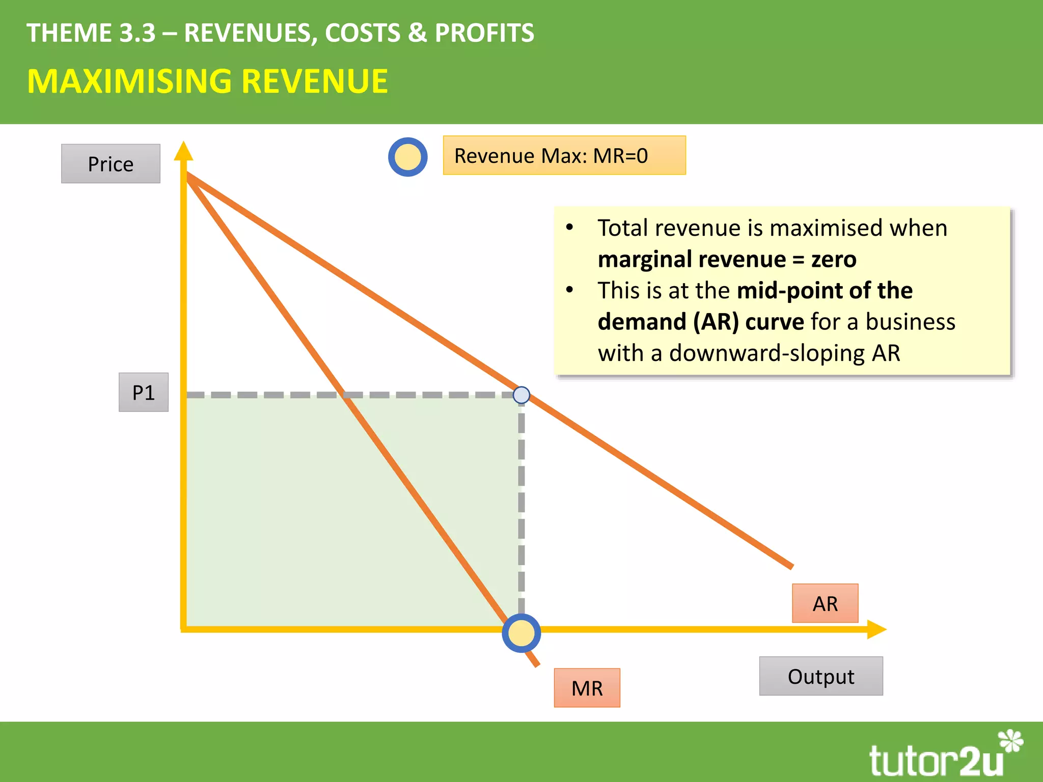
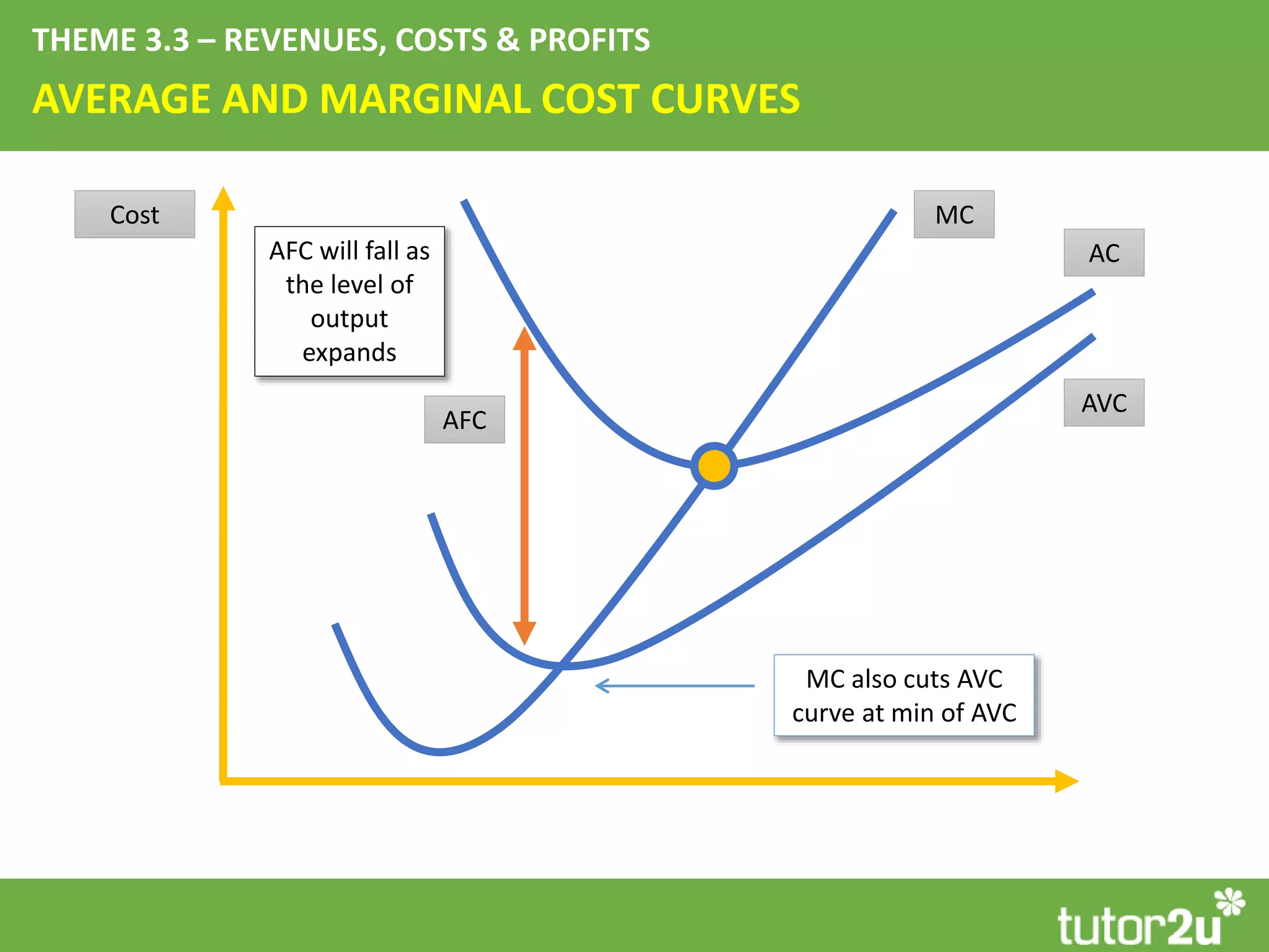
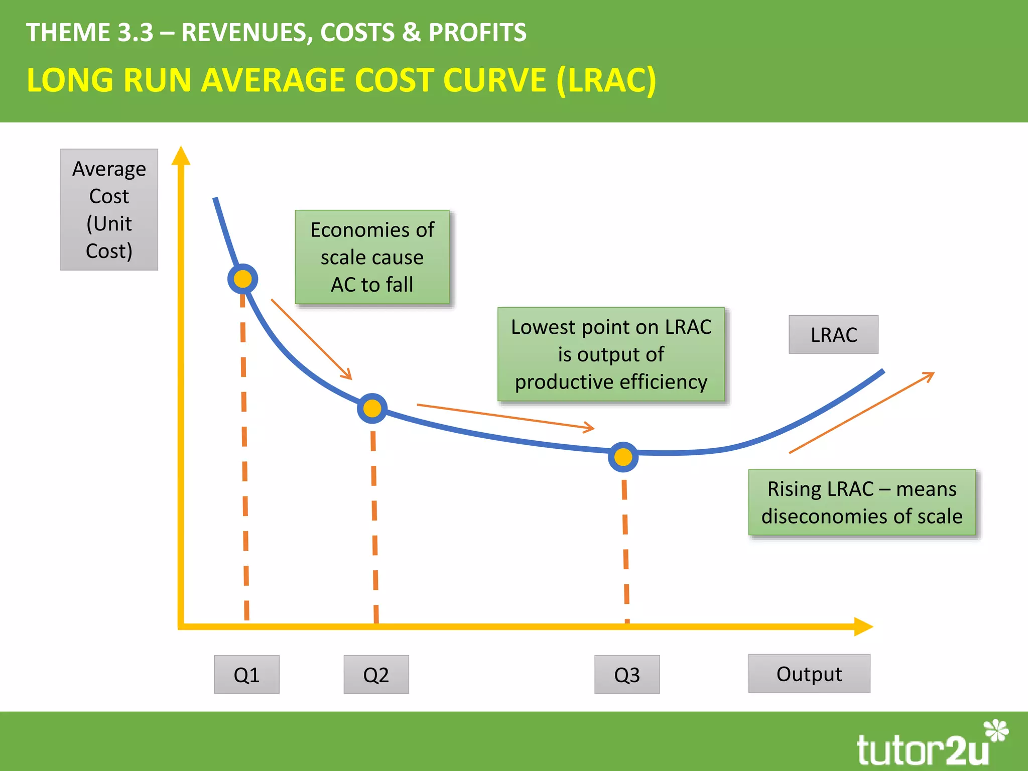
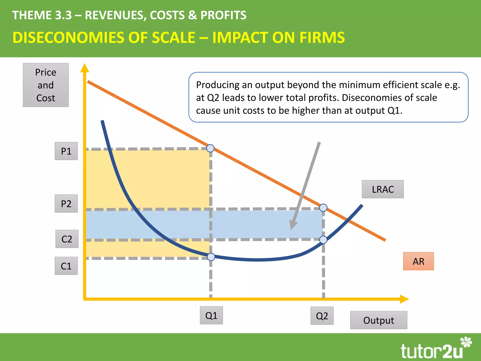
Key Diagrams for Year 2
Microeconomics
Tutor2u, June 2018
THEME 3.2 - BUSINESS OBJECTIVES
SALES REVENUE MAXIMISATION
MC
Price
and
Cost
Output
AC
MR
AR
Profit Max: MC=MR
Revenue Max: MR=0
P1
C1
Total Revenue
THEME 3.2 - BUSINESS OBJECTIVES
SALES MAXIMISATION
MC
Price
and
Cost
Output
AC
MR
AR
Profit Max: MC=MR
Sales Max is at an output where AR=AC
At this output, normal profits are made
P1
Q1
SATISFICING
THEME 3.2 - BUSINESS OBJECTIVES
MC
Price
and
Cost
Output
AC
MR
AR
Possible satisficing price
P1
Q1 Q2
P2
C2
MAXIMISING REVENUE
THEME 3.3 – REVENUES, COSTS & PROFITS
Price
Output
MR
AR
Revenue Max: MR=0
• Total revenue is maximised when
marginal revenue = zero
• This is at the mid-point of the
demand (AR) curve for a business
with a downward-sloping AR
P1
THEME 3.3 – REVENUES, COSTS & PROFITS
PRICE TAKERS AND PRICE MAKERS
Price
Output
Price
Output
AR = MR
AR
MR
Price takers accept the
ruling market price and sell
each unit at the same
price. (AR=MR)
Price makers have
some pricing power
and will face a
downward sloping AR
curve; MR will be
below AR
AVERAGE AND MARGINAL COST CURVES
THEME 3.3 – REVENUES, COSTS & PROFITS
MCCost
AC
AVC
AFC
AFC will fall as
the level of
output
expands
MC also cuts AVC
curve at min of AVC
AVERAGE AND MARGINAL COST CURVES
THEME 3.3 – REVENUES, COSTS & PROFITS
MCCost
AC
AVC
AFC
AFC will fall as
the level of
output
expands
MC also cuts AVC
curve at min of AVC
THEME 3.3 – REVENUES, COSTS & PROFITS
LONG RUN AVERAGE COST CURVE (LRAC)
Q1
Average
Cost
(Unit
Cost)
Output
LRAC
Q2 Q3
Economies of
scale cause
AC to fall
Lowest point on LRAC
is output of
productive efficiency
Rising LRAC – means
diseconomies of scale
THEME 3.3 – REVENUES, COSTS & PROFITS
DISECONOMIES OF SCALE – IMPACT ON FIRMS
Q1
Price
and
Cost
Output
AR
P2
C1
Q2
P1
LRAC
C2
Producing an output beyond the minimum efficient scale e.g.
at Q2 leads to lower total profits. Diseconomies of scale
cause unit costs to be higher than at output Q1.
THEME 3.4 – MARKET STRUCTURES
ALLOCATIVE EFFICIENCY
Price
Quantity
Demand
Supply
P
Q
R
S
T
O
Producer
surplus
Consumer
surplus
Allocative efficiency is at
an output which
maximizes total consumer
welfare
At the market equilibrium
price, consumer and
producer surplus is
maximized – at this
output, economic welfare
is maximized.
THEME 3.4 – MARKET STRUCTURES
PERFECT COMPETITION – SHORT RUN
Price,
Cost
Output
Price,
Cost
Output
Market Supply and
Demand
Revenues, Costs and Profits for a
Competitive Firm
D
S
AC
MC
P1
AR=MR
Q1
C1
Supernormal
profits
THEME 3.4 – MARKET STRUCTURES
PERFECT COMPETITION – LONG RUN ADJUSTMENT
Price,
Cost
Output
Price,
Cost
Output
Market Supply and
Demand
Revenues, Costs and Profits for a
Competitive Firm
D
S1
AC
MC
P1
AR1=MR1
S2
P2
AR2=MR2
Q2
THEME 3.4 – MARKET STRUCTURES
SHUT-DOWN PRICE
AC
AVC
P1: Price = average
cost, normal profits
made
P2: Price = average
variable cost
P=Min AVC is the shut
down price for a
competitive firm in
short run
Price
MC
P1
P2
THEME 3.4 – MARKET STRUCTURES
MONOPOLISTIC COMPETITION – SHORT RUN
MC
Price
and
Cost
Output
AC
MR
AR
P1
Q1
C1
Supernormal
Profit
THEME 3.4 – MARKET STRUCTURES
MONOPOLISTIC COMPETITION – LONG RUN
MC
Price
and
Cost
Output
AC
MR2
AR2
P2
Q2
In the long run equilibrium,
average revenue is tangential
to AC – meaning normal profits
are being made because P=AC
THEME 3.4 – MARKET STRUCTURES
MONOPOLY PRICE AND OUTPUT
MC
Price
and
Cost
Output
AC
MRProfit Max: MC=MR
P1
Q1
C1
Supernormal Profit
AR
The average revenue
is much higher than
the unit cost at
output Q1
The monopoly is
a price-maker
although it is
also constrained
by their demand
curve
NATURAL MONOPOLY
THEME 3.4 – MARKET STRUCTURES
Price
and
Cost
Output
LRAC
LRMC
MR
AR
P1
C1
A natural monopoly there there are high fixed
costs involved in supplying a good or service such
that the long run average cost curve may fall
continuously as output increases in the long run.
Marginal cost is less than average cost. This helps
to drive down average cost as output increases.
Q1
THEME 3.4 – MARKET STRUCTURES
3RD DEGREE PRICE DISCRIMINATION
Price
Output
Price
Output
AR
AR
MRMR
MC MC
Elastic demand – consumers
responsive to small price
changes
Inelastic demand – high
willingness/ ability to
pay
P1
Q1
P2
Q2
C1
THEME 3.4 – MARKET STRUCTURES
PEAK AND OFF-PEAK PRICING
Price
Output
MR off peak
AR off peak
MC
P off-peak
Q1 Q2
P peak
MR peak
AR peak
At off-peak times, market
demand is low and firms
will have spare capacity
PRICES AND PROFITS IN CONTESTABLE MARKETS
THEME 3.4 – MARKET STRUCTURES
MC
Price
and
Cost
Output
AC
MR
P1
Q1
C1 AR
Q2
P2
Profit maximising
price
Price where normal
profits are made
Threat of competition likely to cause
firms to price at P2 rather than P1
CONTROLLING MARKET POWER – PRICE CAPPING
THEME 3.6 – GOVERNMENT INTERVENTION
MC
Price
and
Cost
Output
AC
MR
AR
P1
Q1
C1
Supernormal Profit
Capped
Price
Q2
C2
At a capped price, the monopolist can make
a profit, but supernormal profit will be lower.
KINKED DEMAND CURVE MODEL
4.1.5.5 OLIGOPOLY
Price
and
Cost
Output
AR1
P1
AR2
Cutting price below P1: Likely reaction of other firms is to
follow the price reduction. Demand likely to be relatively
inelastic – little benefit in terms of extra sales and total revenue
Q1
P2
Q2
P3
Q3
Raising price above P1: Likely reaction of other firms is to hold
their prices. This will cause an elastic demand response and
results in lost sales and falling total revenue
KINKED DEMAND CURVE MODEL – OUTCOME
4.1.5.5 OLIGOPOLY
Price
and
Cost
Output
AR1
Is there a profit maximising equilibrium in this market? In
the diagram here MC1 cuts through the gap in the
marginal revenue curve
MR1
MC1
Kinked demand curve model assumes:
Other firms will follow if prices are cut
Firms will not follow if prices rise
MC2
One of the key predictions of the
kinked demand curve model is that
prices will be rigid or “sticky” even
when there is a change in the
marginal costs of supply (this is
assuming that firms in the market are
profit seeking)
ELASTICITY OF LABOUR DEMAND
4.1.6.1 DEMAND FOR LABOUR
Wage
Rate
Employment
LD1
W1
W2
W3
E1E2
LD1 is elastic – i.e.
employment is sensitive to
a changing wages
Wage
Rate
Employment
LD2
W1
W3
E1E3
LD2 is inelastic – i.e. a large rise in wages
causes only a small fall in employment
ELASTICITY OF LABOUR SUPPLY
4.1.6.2 INFLUENCES ON SUPPLY OF LABOUR
Wage
Rate
Employment
LS1
W1
W2
E1 E2
Wage
Rate
Employment
LS2
W1
W2
E1 E2
In relatively lower-skilled jobs, the
labour supply is elastic because a
pool of labour is available to be
employed at a fairly constant market
wage rate.
Where jobs require specific skills and
training, the labour supply will be
more inelastic.
EQUILIBRIUM WAGES
4.1.6.2 INFLUENCES ON SUPPLY OF LABOUR
Wage
Rate
Employment
LS1
W1
E1
Wage
Rate
LS1
W1
W2
E1 E2
LD1
LD1
An outward shift of
labour demand
LD2
Employment
LOW PAY AND THE UK MINIMUM WAGE
4.1.6.6 THE NATIONAL MINIMUM WAGE
Wage
Rate
Employment
LS1
W1
E1
Wage
Rate
EmploymentE2 E3
LD1
LD1
W1
LS1
W2 Min Wage
The free market wage is W1 with employment level of E1. If a minimum wage of W2 is
introduced, then employment contracts to E2 and the supply of labour expands to E3
MONOPSONY EMPLOYER – WAGE ANALYSIS
4.1.6.4 IMPERFECTLY COMPETITIVE LABOUR MARKET
Wage
Rate
Employment
Labour Supply (=
ACL)
W1
E1
• Profit maximising
employment level
is where
MCL=MRPL i.e. E2
number of people
are employed
• Their marginal
revenue product is
valued at W2
• Monopsony power
of the employer
allows them to pay
a wage rate W3
Labour Demand =
MRPL
Marginal cost of
labour (MCL)
E2
W2
W3
MONOPSONY EMPLOYER – WAGE ANALYSIS
4.1.6.4 IMPERFECTLY COMPETITIVE LABOUR MARKET
Wage
Rate
Employment
Labour Supply (=
ACL)
W1
E1
• Monopsony
employer can use
their buying power
to pay a wage lower
than the value of
the marginal
revenue product of
workers employed
at E2
• Monopsony power
can lead to
exploitation of
employed workers
Labour Demand =
MRPL
Marginal cost of
labour (MCL)
E2
W2
W3
Total
wages
Lost wages from
under-payment
MONOPSONY POWER WITH MINIMUM WAGE
4.1.6.4 IMPERFECTLY COMPETITIVE LABOUR MARKET
• A minimum wage
is enforced in the
labour market.
• This means that
the marginal cost
of employing
labour is constant
up to employment
level E4
• Thereafter the MC
and AC of
employing
workers diverges
Wage
Rate
Employment
Labour Supply (=
ACL)
Labour Demand =
MRPL
E2
W3
Total
wages
E4
MCL
MCL with min wage
Wmin
MONOPSONY POWER WITH MINIMUM WAGE
4.1.6.4 IMPERFECTLY COMPETITIVE LABOUR MARKET
• The new profit
maximising level
of employment
with the minimum
wage is now at E3
– which is a higher
employment level
and a higher wage
than with the
previous wage
paid by the
monopsony
employer.
Wage
Rate
Employment
Labour Supply (=
ACL)Wmin
Labour Demand =
MRPL
E2
W3
Total
wages
E4
MCL
MCL with min wage
E3
TRADE UNIONS – WAGE AND JOBS ANALYSIS
4.1.6.5 INFLUENCE OF TRADE UNIONS
Wage
Rate
Employment
Labour Supply
W1
E1
Labour Demand
Union negotiated
wage
W2
E2
Higher wage income from
union collective bargaining
Lost wage income
from contraction
in employment
• Unions will have more
success in raising
wages for their
members if the
demand for labour is
relatively wage
inelastic
• Unions also more
influential when they
represent a high % of
all workers in a given
industry/occupation
• Pay might also rise if
unions and employers
agree a pay deal based
on better productivity
THE LORENZ CURVE
4.1.7.1 DISTRIBUTION OF INCOME AND WEALTH
Cumulative % of Income100%
50%
0%
Line of Equality
Lorenz Curve
(High Inequality)
Lorenz Curve (Low
Inequality)
Households by Income – Quintile DistributionPoorest Richest
The Lorenz
Curve gives a
visual
interpretation
of income or
wealth
inequality.
The diagonal
line shows a
situation of
perfect equality
of income i.e.
50% of
population has
50% of income
Key Diagrams for Year 2
Microeconomics
Tutor2u, June 2018

Key Diagrams for Year 2 Microeconomics

  • 1.
    Key Diagrams forYear 2 Microeconomics Tutor2u, June 2018
  • 2.
    THEME 3.2 -BUSINESS OBJECTIVES SALES REVENUE MAXIMISATION MC Price and Cost Output AC MR AR Profit Max: MC=MR Revenue Max: MR=0 P1 C1 Total Revenue
  • 3.
    THEME 3.2 -BUSINESS OBJECTIVES SALES MAXIMISATION MC Price and Cost Output AC MR AR Profit Max: MC=MR Sales Max is at an output where AR=AC At this output, normal profits are made P1 Q1
  • 4.
    SATISFICING THEME 3.2 -BUSINESS OBJECTIVES MC Price and Cost Output AC MR AR Possible satisficing price P1 Q1 Q2 P2 C2
  • 5.
    MAXIMISING REVENUE THEME 3.3– REVENUES, COSTS & PROFITS Price Output MR AR Revenue Max: MR=0 • Total revenue is maximised when marginal revenue = zero • This is at the mid-point of the demand (AR) curve for a business with a downward-sloping AR P1
  • 6.
    THEME 3.3 –REVENUES, COSTS & PROFITS PRICE TAKERS AND PRICE MAKERS Price Output Price Output AR = MR AR MR Price takers accept the ruling market price and sell each unit at the same price. (AR=MR) Price makers have some pricing power and will face a downward sloping AR curve; MR will be below AR
  • 7.
    AVERAGE AND MARGINALCOST CURVES THEME 3.3 – REVENUES, COSTS & PROFITS MCCost AC AVC AFC AFC will fall as the level of output expands MC also cuts AVC curve at min of AVC
  • 8.
    AVERAGE AND MARGINALCOST CURVES THEME 3.3 – REVENUES, COSTS & PROFITS MCCost AC AVC AFC AFC will fall as the level of output expands MC also cuts AVC curve at min of AVC
  • 9.
    THEME 3.3 –REVENUES, COSTS & PROFITS LONG RUN AVERAGE COST CURVE (LRAC) Q1 Average Cost (Unit Cost) Output LRAC Q2 Q3 Economies of scale cause AC to fall Lowest point on LRAC is output of productive efficiency Rising LRAC – means diseconomies of scale
  • 10.
    THEME 3.3 –REVENUES, COSTS & PROFITS DISECONOMIES OF SCALE – IMPACT ON FIRMS Q1 Price and Cost Output AR P2 C1 Q2 P1 LRAC C2 Producing an output beyond the minimum efficient scale e.g. at Q2 leads to lower total profits. Diseconomies of scale cause unit costs to be higher than at output Q1.
  • 11.
    THEME 3.4 –MARKET STRUCTURES ALLOCATIVE EFFICIENCY Price Quantity Demand Supply P Q R S T O Producer surplus Consumer surplus Allocative efficiency is at an output which maximizes total consumer welfare At the market equilibrium price, consumer and producer surplus is maximized – at this output, economic welfare is maximized.
  • 12.
    THEME 3.4 –MARKET STRUCTURES PERFECT COMPETITION – SHORT RUN Price, Cost Output Price, Cost Output Market Supply and Demand Revenues, Costs and Profits for a Competitive Firm D S AC MC P1 AR=MR Q1 C1 Supernormal profits
  • 13.
    THEME 3.4 –MARKET STRUCTURES PERFECT COMPETITION – LONG RUN ADJUSTMENT Price, Cost Output Price, Cost Output Market Supply and Demand Revenues, Costs and Profits for a Competitive Firm D S1 AC MC P1 AR1=MR1 S2 P2 AR2=MR2 Q2
  • 14.
    THEME 3.4 –MARKET STRUCTURES SHUT-DOWN PRICE AC AVC P1: Price = average cost, normal profits made P2: Price = average variable cost P=Min AVC is the shut down price for a competitive firm in short run Price MC P1 P2
  • 15.
    THEME 3.4 –MARKET STRUCTURES MONOPOLISTIC COMPETITION – SHORT RUN MC Price and Cost Output AC MR AR P1 Q1 C1 Supernormal Profit
  • 16.
    THEME 3.4 –MARKET STRUCTURES MONOPOLISTIC COMPETITION – LONG RUN MC Price and Cost Output AC MR2 AR2 P2 Q2 In the long run equilibrium, average revenue is tangential to AC – meaning normal profits are being made because P=AC
  • 17.
    THEME 3.4 –MARKET STRUCTURES MONOPOLY PRICE AND OUTPUT MC Price and Cost Output AC MRProfit Max: MC=MR P1 Q1 C1 Supernormal Profit AR The average revenue is much higher than the unit cost at output Q1 The monopoly is a price-maker although it is also constrained by their demand curve
  • 18.
    NATURAL MONOPOLY THEME 3.4– MARKET STRUCTURES Price and Cost Output LRAC LRMC MR AR P1 C1 A natural monopoly there there are high fixed costs involved in supplying a good or service such that the long run average cost curve may fall continuously as output increases in the long run. Marginal cost is less than average cost. This helps to drive down average cost as output increases. Q1
  • 19.
    THEME 3.4 –MARKET STRUCTURES 3RD DEGREE PRICE DISCRIMINATION Price Output Price Output AR AR MRMR MC MC Elastic demand – consumers responsive to small price changes Inelastic demand – high willingness/ ability to pay P1 Q1 P2 Q2 C1
  • 20.
    THEME 3.4 –MARKET STRUCTURES PEAK AND OFF-PEAK PRICING Price Output MR off peak AR off peak MC P off-peak Q1 Q2 P peak MR peak AR peak At off-peak times, market demand is low and firms will have spare capacity
  • 21.
    PRICES AND PROFITSIN CONTESTABLE MARKETS THEME 3.4 – MARKET STRUCTURES MC Price and Cost Output AC MR P1 Q1 C1 AR Q2 P2 Profit maximising price Price where normal profits are made Threat of competition likely to cause firms to price at P2 rather than P1
  • 22.
    CONTROLLING MARKET POWER– PRICE CAPPING THEME 3.6 – GOVERNMENT INTERVENTION MC Price and Cost Output AC MR AR P1 Q1 C1 Supernormal Profit Capped Price Q2 C2 At a capped price, the monopolist can make a profit, but supernormal profit will be lower.
  • 23.
    KINKED DEMAND CURVEMODEL 4.1.5.5 OLIGOPOLY Price and Cost Output AR1 P1 AR2 Cutting price below P1: Likely reaction of other firms is to follow the price reduction. Demand likely to be relatively inelastic – little benefit in terms of extra sales and total revenue Q1 P2 Q2 P3 Q3 Raising price above P1: Likely reaction of other firms is to hold their prices. This will cause an elastic demand response and results in lost sales and falling total revenue
  • 24.
    KINKED DEMAND CURVEMODEL – OUTCOME 4.1.5.5 OLIGOPOLY Price and Cost Output AR1 Is there a profit maximising equilibrium in this market? In the diagram here MC1 cuts through the gap in the marginal revenue curve MR1 MC1 Kinked demand curve model assumes: Other firms will follow if prices are cut Firms will not follow if prices rise MC2 One of the key predictions of the kinked demand curve model is that prices will be rigid or “sticky” even when there is a change in the marginal costs of supply (this is assuming that firms in the market are profit seeking)
  • 25.
    ELASTICITY OF LABOURDEMAND 4.1.6.1 DEMAND FOR LABOUR Wage Rate Employment LD1 W1 W2 W3 E1E2 LD1 is elastic – i.e. employment is sensitive to a changing wages Wage Rate Employment LD2 W1 W3 E1E3 LD2 is inelastic – i.e. a large rise in wages causes only a small fall in employment
  • 26.
    ELASTICITY OF LABOURSUPPLY 4.1.6.2 INFLUENCES ON SUPPLY OF LABOUR Wage Rate Employment LS1 W1 W2 E1 E2 Wage Rate Employment LS2 W1 W2 E1 E2 In relatively lower-skilled jobs, the labour supply is elastic because a pool of labour is available to be employed at a fairly constant market wage rate. Where jobs require specific skills and training, the labour supply will be more inelastic.
  • 27.
    EQUILIBRIUM WAGES 4.1.6.2 INFLUENCESON SUPPLY OF LABOUR Wage Rate Employment LS1 W1 E1 Wage Rate LS1 W1 W2 E1 E2 LD1 LD1 An outward shift of labour demand LD2 Employment
  • 28.
    LOW PAY ANDTHE UK MINIMUM WAGE 4.1.6.6 THE NATIONAL MINIMUM WAGE Wage Rate Employment LS1 W1 E1 Wage Rate EmploymentE2 E3 LD1 LD1 W1 LS1 W2 Min Wage The free market wage is W1 with employment level of E1. If a minimum wage of W2 is introduced, then employment contracts to E2 and the supply of labour expands to E3
  • 29.
    MONOPSONY EMPLOYER –WAGE ANALYSIS 4.1.6.4 IMPERFECTLY COMPETITIVE LABOUR MARKET Wage Rate Employment Labour Supply (= ACL) W1 E1 • Profit maximising employment level is where MCL=MRPL i.e. E2 number of people are employed • Their marginal revenue product is valued at W2 • Monopsony power of the employer allows them to pay a wage rate W3 Labour Demand = MRPL Marginal cost of labour (MCL) E2 W2 W3
  • 30.
    MONOPSONY EMPLOYER –WAGE ANALYSIS 4.1.6.4 IMPERFECTLY COMPETITIVE LABOUR MARKET Wage Rate Employment Labour Supply (= ACL) W1 E1 • Monopsony employer can use their buying power to pay a wage lower than the value of the marginal revenue product of workers employed at E2 • Monopsony power can lead to exploitation of employed workers Labour Demand = MRPL Marginal cost of labour (MCL) E2 W2 W3 Total wages Lost wages from under-payment
  • 31.
    MONOPSONY POWER WITHMINIMUM WAGE 4.1.6.4 IMPERFECTLY COMPETITIVE LABOUR MARKET • A minimum wage is enforced in the labour market. • This means that the marginal cost of employing labour is constant up to employment level E4 • Thereafter the MC and AC of employing workers diverges Wage Rate Employment Labour Supply (= ACL) Labour Demand = MRPL E2 W3 Total wages E4 MCL MCL with min wage Wmin
  • 32.
    MONOPSONY POWER WITHMINIMUM WAGE 4.1.6.4 IMPERFECTLY COMPETITIVE LABOUR MARKET • The new profit maximising level of employment with the minimum wage is now at E3 – which is a higher employment level and a higher wage than with the previous wage paid by the monopsony employer. Wage Rate Employment Labour Supply (= ACL)Wmin Labour Demand = MRPL E2 W3 Total wages E4 MCL MCL with min wage E3
  • 33.
    TRADE UNIONS –WAGE AND JOBS ANALYSIS 4.1.6.5 INFLUENCE OF TRADE UNIONS Wage Rate Employment Labour Supply W1 E1 Labour Demand Union negotiated wage W2 E2 Higher wage income from union collective bargaining Lost wage income from contraction in employment • Unions will have more success in raising wages for their members if the demand for labour is relatively wage inelastic • Unions also more influential when they represent a high % of all workers in a given industry/occupation • Pay might also rise if unions and employers agree a pay deal based on better productivity
  • 34.
    THE LORENZ CURVE 4.1.7.1DISTRIBUTION OF INCOME AND WEALTH Cumulative % of Income100% 50% 0% Line of Equality Lorenz Curve (High Inequality) Lorenz Curve (Low Inequality) Households by Income – Quintile DistributionPoorest Richest The Lorenz Curve gives a visual interpretation of income or wealth inequality. The diagonal line shows a situation of perfect equality of income i.e. 50% of population has 50% of income
  • 35.
    Key Diagrams forYear 2 Microeconomics Tutor2u, June 2018