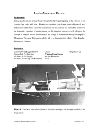
1. The Impulse-Momentum Theorem states that the net impulse acting on an object is equal to the change in momentum of the object. 2. In the experiment, a glider collides with a force sensor on an air track to test the Impulse-Momentum Theorem. The initial and final velocities are measured with a photogate and the force over time is measured with a wireless force sensor. 3. The data is analyzed by calculating the impulse, change in momentum, and comparing the two to test the validity of the Impulse-Momentum Theorem.

1. Impulse-Momentum Theorem
Introduction
During a collision, the contact force between the objects participating in the collision is not
constant, but varies with time. Thus the accelerations experienced by the objects will also
be functions of the time. Since the accelerations are not constant we will not be able to use
the kinematics equations of motion to analyze this situation. Instead, we will rely upon the
concept of impulse and its relationship to the change in momentum through the Impulse-
Momentum Theorem. The purpose of this lab is to determine the validity of the Impulse-
Momentum Theorem.
Equipment
Computer with Logger Pro SW Glider Ringstands (2)
Vernier Lab Pro Interface Wireless Force Sensor
Air Track & Air Supply Vernier Photogate
Air Track Accessory Kit (Bumpers) Scale
Figure 1. Overhead view of the glider as it is about to impact the bumper attached to the
force sensor.
13f Impulse-Momentum-Wireless 3-3-09 -1- Revised 10-11-07

2. Terminology
Impulse: (Area under the F-vs-t graph) J = F ∆t
Net Impulse: (Area under the Fnet-vs-t graph) J net = Fnet ∆t
Momentum: p = mv
Change in Momentum: ∆p = mv − mv0
Theory
The easiest way to analyze this collision situation is to make a graph of the force versus
time. The impulse of this force over a given time interval is the area under the curve over
the same time interval. The time interval will usually be the interval during which the
force acts. If the force were constant, then the graph of the force versus time would be a
horizontal line and the area under the curve would be the value of the constant force
multiplied by the time interval. However, since the force varies with time, we need to use
the average force, over the time interval.
The net impulse acting on an object is the vector sum of all of the impulses that act
on the object, or alternatively it is the area under the curve of the graph of the net force
acting on the object versus time. The Impulse-Momentum Theorem states that the net
impulse acting on the object is also equal to the change in the momentum of the object.
J net = Fnet ∆t = ∆p
p = mv & ∆p = mv − mv0
In this lab we will produce a one-dimensional elastic collision between a glider,
riding on an air track, and a stationary force sensor. The photogate timer will record the
initial and final velocities and the force sensor will record the force as a function of time.
We will then use this data to determine the validity of the Impulse-Momentum Theorem.
13f Impulse-Momentum-Wireless 3-3-09 -2- Revised 10-11-07

3. Equipment Set Up Procedure
Computer – Turn on the computer and click on the Logger Pro icon. To create the
data collection file for this experiment click on the Experiment menu and then click on the
Set Up Sensors menu item. Select Show All Interfaces. At present there are no sensors
attached to the Lab Pro Interface. For the digital interface select the photogate and drag it to
the digital CH1. Select the “Gate Timer” function for the photogate and set the “Flag
Length” or “Photogate Distance” of the cylindrical object (in meters) that you are using
as a flag.
Setting up your WDSS
1. Turn on the WDSS. Note the name on the label of the device.
2. Make sure Bluetooth is activated on your computer. Some computers have Bluetooth
built into them. If that is the case, make sure Bluetooth is turned on.
3. Establish a wireless connection with the WDSS.
a. Choose Connect Interface from the Experiment menu. Choose Wireless and then
Scan for Wireless Device.
b. There will be a short delay while Logger Pro attempts to establish a connection. If
the WDSS is not found, try scanning again.
c. A dialog box will appear showing your WDSS on the list of available devices.
Select your WDSS device and then click OK . Once a connection is made, the two
LEDs on the WDSS will be lit green.
Choose Data Collection from the Experiment menu. Adjust the data collection
experiment length to 10 seconds with a sampling rate of 200 samples/second.
Save the set up as MyImpulse_Temp on the Desktop. The Data Interval should be 0.01 or
0.02 seconds.
Air Track Procedure – Turn on the air track air supply and adjust the volume of the
air flow so that the glider rides freely on a cushion of air. To level the air track place the
glider at the center of the track and then adjust the feet on the air track until any motion of
the glider is minimized.
13f Impulse-Momentum-Wireless 3-3-09 -3- Revised 10-11-07

4. Glider Procedure –For a cylindrical “flag” its diameter is the length to be used.
There is no orientation problem with the cylindrical flag. The “length of the flag” will be
determined by measuring it with the calipers. You should enter this value of the length into
the computer
To Enter the Flag Length into the computer: Click on the Experiment menu and
click on the Set Up Sensors menu item. Then select Show All Interfaces. Click on the
Photogate icon and select “Set Distance or Length.” Then enter the “Flag Length” and
click OK.
Bumpers – The bumpers are mounted on each end of the glider (for balance) and on
the end of the force sensor. If there are only two (2) bumpers available then another object
equal in mass to the bumper needs to be mounter on the other end of the glider.
Photogate Placement Procedure - We will use a photogate to measure the initial
velocity of the glider prior to the collision as well as the final velocity of the glider after the
collision. Place the photogate as close to the force sensor as possible so that the glider
completely clears the photogate before it comes into contact with the force sensor. Check
to make sure that the bumper on the glider does not come into contact with the photogate.
Wireless Force Sensor Procedure – To ensure the integrity of your data you will
need to make sure that the force sensor does not move during the collision. Do not send the
glider into the force sensor too hard, if the bumper bracket on the glider and the one on the
force sensor touch each other the data will not be accurate and the run will have to be
repeated.
Final Alignment Check - You will be using one of the cylindrical objects as the
flag. Orientation is not a problem, but if the upper portion of the cylinder is a blade
structure make sure the photogate height is adjusted so that the beam is broken by the
CYLINDRICAL portion and NOT the BLADE portion. The glider bumper should not
strike anything as it passes through the photogate and it should hit the bumper on the force
sensor dead center. The photogate should be centered over the air track and the beam path
aligned perpendicular to the length of the track. The photogate should be located far
enough from the force sensor so that the glider clears the gate prior to hitting the force
sensor.
13f Impulse-Momentum-Wireless 3-3-09 -4- Revised 10-11-07

5. Experimental Procedure
Precision - All observations should be recorded to 3 significant figures. You should carry
3 significant figures in all of your calculations as well.
1. To begin a run first zero the force sensor by clicking the Zero button and then click the
Collect button to start the data collection. Gently push the glider to launch it toward
the force sensor. You should have finished pushing the glider well before it enters the
photogate. The brackets for the bumpers should not touch one another. Let the
measurement run all the way out until the end of the collection time and the Stop
button disappears and the Collect button returns.
2. TURN OFF the sensor between runs to conserve battery power.
3. On the Force versus Time graph locate the non-zero region of the graph and highlight it
by clicking and dragging the cursor across the region. Click the Integral button and
record the value of the integral, which is simply the area under the curve, as the Net
Impulse in the Data Table.
4. Locate and record the initial and final velocities that occurred before and after the
collision. Don’t forget to include the directions for these vector quantities.
5. Record the time interval for the collision as well as the maximum value of the force.
Determine these by using the inspection function with the Force versus Time graph.
6. Repeat this process five (5) more times with the first bumper. Print a representative
graph for one of these runs. Measure the mass of your glider using the scale.
Data Analysis
• Calculate the following quantities for each run: ∆p and compare it through a percent
difference with the Jnet.
• Then calculate the average net force for each run by Fnet = J net ÷ ∆t
• Plot a graph (X-Y Scatter) of Jnet (y-axis) versus ∆p (x-axis). Determine the slope, y-
intercept and correlation coefficient of the trendline. Use the LINEST Excel function to
determine the uncertainties in these quantities.
13f Impulse-Momentum-Wireless 3-3-09 -5- Revised 10-11-07

6. Questions
1. In this lab we neglected friction because we have significantly reduced its affect by the
use of an air track. If friction were present what would be its affect on the values of the
velocities? How would this affect the momentum values? What would this do to the
value of the momentum change as it compares to the net impulse?
2. In general, how do the average force and the maximum force for each run compare to
one another?
3. In general what were the differences that you observed between the two bumpers that
were used? Your description should involve things like the differences in the graphs,
the amount of time of the collisions, as well as the average and maximum force
involved in the collision.
4. Within reasonable limits for experimental uncertainty were you able to verify the
Impulse-Momentum Theorem?
Lab Report
Follow the instructions in the document “ Format for Formal Lab Reports.”
13f Impulse-Momentum-Wireless 3-3-09 -6- Revised 10-11-07

7. Data Tables
Diameter of cylindrical flag = _______________(m)
Bumper #1 – Data Table
Mass of glider = ________________(kg)
Run Jnet ∆t Fmax V0 p0 V p
(Ns) (s) (N) (m/s) (kg*m/s) (m/s) (kg*m/s)
1
2
3
4
5
6
Bumper #1 – Analysis Table
Run p0 p ∆p Favg
(kg*m/s) (kg*m/s) (kg*m/s) (N)
1
2
3
4
5
6
13f Impulse-Momentum-Wireless 3-3-09 -7- Revised 10-11-07