11 - 3 Experiment 11 Simple Harmonic Motion Questions How are swinging pendulums and masses on springs related? Why are these types of problems so important in Physics? What is a spring’s force constant and how can you measure it? What is linear regression? How do you use graphs to ascertain physical meaning from equations? Again, how do you compare two numbers, which have errors? Note: This week all students must write a very brief lab report during the lab period. It is due at the end of the period. The explanation of the equations used, the introduction and the conclusion are not necessary this week. The discussion section can be as little as three sentences commenting on whether the two measurements of the spring constant are equivalent given the propagated errors. This mini-lab report will be graded out of 50 points Concept When an object (of mass m) is suspended from the end of a spring, the spring will stretch a distance x and the mass will come to equilibrium when the tension F in the spring balances the weight of the body, when F = - kx = mg. This is known as Hooke's Law. k is the force constant of the spring, and its units are Newtons / meter. This is the basis for Part 1. In Part 2 the object hanging from the spring is allowed to oscillate after being displaced down from its equilibrium position a distance -x. In this situation, Newton's Second Law gives for the acceleration of the mass: Fnet = m a or The force of gravity can be omitted from this analysis because it only serves to move the equilibrium position and doesn’t affect the oscillations. Acceleration is the second time- derivative of x, so this last equation is a differential equation. To solve: we make an educated guess: Here A and w are constants yet to be determined. At t = 0 this solution gives x(t=0) = A, which indicates that A is the initial distance the spring stretches before it oscillates. If friction is negligible, the mass will continue to oscillate with amplitude A. Now, does this guess actually solve the (differential) equation? A second time-derivative gives: Comparing this equation to the original differential equation, the correct solution was chosen if w2 = k / m. To understand w, consider the first derivative of the solution: −kx = ma a = − k m ⎛ ⎝ ⎜⎜⎜⎜ ⎞ ⎠ ⎟⎟⎟⎟ x d 2x dt 2 = − k m x x(t) = A cos(ωt) d 2x(t) dt 2 = −Aω2 cos(ωt) = −ω2x(t) James Gering Florida Institute of Technology 11 - 4 Integrating gives We assume the object completes one oscillation in a certain period of time, T. This helps set the limits of integration. Initially, we pull the object a distance A from equilibrium and release it. So at t = 0 and x = A. (one.

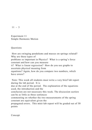
1. 11 - 3
Experiment 11
Simple Harmonic Motion
Questions
How are swinging pendulums and masses on springs related?
Why are these types of
problems so important in Physics? What is a spring’s force
constant and how can you measure
it? What is linear regression? How do you use graphs to
ascertain physical meaning from
equations? Again, how do you compare two numbers, which
have errors?
Note: This week all students must write a very brief lab report
during the lab period. It is
due at the end of the period. The explanation of the equations
used, the introduction and the
conclusion are not necessary this week. The discussion section
can be as little as three sentences
commenting on whether the two measurements of the spring
constant are equivalent given the
propagated errors. This mini-lab report will be graded out of 50
points
Concept

2. When an object (of mass m) is suspended from the end of a
spring, the spring will stretch
a distance x and the mass will come to equilibrium when the
tension F in the spring balances the
weight of the body, when F = - kx = mg. This is known as
Hooke's Law. k is the force constant
of the spring, and its units are Newtons / meter. This is the
basis for Part 1.
In Part 2 the object hanging from the spring is allowed to
oscillate after being displaced
down from its equilibrium position a distance -x. In this
situation, Newton's Second Law gives
for the acceleration of the mass:
Fnet = m a or
The force of gravity can be omitted from this analysis because
it only serves to move the
equilibrium position and doesn’t affect the oscillations.
Acceleration is the second time-
derivative of x, so this last equation is a differential equation.
To solve: we make an educated guess:
Here A and w are constants yet to be determined. At t = 0 this
solution gives x(t=0) = A,
which indicates that A is the initial distance the spring stretches
before it oscillates. If friction is
negligible, the mass will continue to oscillate with amplitude A.
Now, does this guess actually
solve the (differential) equation? A second time-derivative

3. gives:
Comparing this equation to the original differential equation,
the correct solution was
chosen if w2 = k / m. To understand w, consider the first
derivative of the solution:
−kx = ma
a = −
k
m
⎛
⎝
⎜⎜⎜⎜
⎞
⎠
⎟⎟⎟⎟
x
d 2x
dt 2
= −
k
m
x x(t) = A cos(ωt)

4. d 2x(t)
dt 2
= −Aω2 cos(ωt) = −ω2x(t)
James Gering
Florida Institute of Technology
11 - 4
Integrating gives
We assume the object completes one oscillation in a certain
period of time, T. This helps
set the limits of integration. Initially, we pull the object a
distance A from equilibrium and
release it. So at t = 0 and x = A. (one-quarter of the total
period later) the object passes the
equilibrium (x=0) position.
This integration yields: Canceling the A’s and w’s
and evaluating these limits gives:
or, and adding 1 to both sides gives cos [ (wT / 4) ] = 0

5. The cosine is zero only when its argument is p/2 radians. Hence
this last equation implies that
and rearranging gives
Finally, it is clear that w is indeed the angular frequency of the
object as it oscillates up and
down. Earlier it was found that w2 = k/m. Putting these two
relations for w together yields:
or
This last equation is only valid if the mass of the spring is
negligible compared to m. In
the case of a massive spring, the actual mass that oscillates
includes a portion of the mass of the
spring - the upper part of the spring is stretched by the lower
part. This suggests that an
“effective mass” meff should be added to m to give:
or after squaring both sides
Writing this last equation this way emphasizes the equation is
of the form of y = Ax + B, if y is
taken as T2 and x is taken as the mass m. Therefore, a graph of
T2 versus mass will yield a
straight line with a physically meaningful slope and y-intercept.

6. v(t) =
dx(t)
dt
= −Aωsin(ωt)
dx = Aω sin(ωt)dt
t=0
t=T /4
∫x =A
x =0
∫
−A = Aω
cos(ωt)
ω
⎡
⎣
⎢
⎤
⎦
⎥
0

7. T /4
−1 = cos(
ωT
4
)−cos(0)
−1 = [cos
ωT
4
⎛
⎝
⎜⎜⎜⎜
⎞
⎠
⎟⎟⎟⎟
−1]
ωT
4
=
π
2
ω =

8. 2π
T
2π
T
⎛
⎝
⎜⎜⎜⎜
⎞
⎠
⎟⎟⎟⎟
2
=
k
m
T = 2π
m
k
⎛
⎝
⎜⎜⎜⎜
⎞

9. ⎠
⎟⎟⎟⎟
1/2
T = 2π
m + m
eff
k
⎛
⎝
⎜⎜⎜⎜⎜
⎞
⎠
⎟⎟⎟⎟⎟
1/2
T 2 =
4π2
k
m +
4π2

10. k
m
eff
James Gering
Florida Institute of Technology
11 - 5
Procedure
Part 0 Evaluations and Assessment
1) Reminder: After this experiment, find some time to use
Canvas to fill out the end-of-
semester course evaluation.
2) (Note: This task may be converted into a Canvas quiz or it
may be something entirely
different. As of this writing, things are in flux.) Instructors
will reserve 35-40 minutes to
administer a diagnostic exam, which is part of the Department’s
year-to-year assessment
of the Physics 1 lecture class (PHY 1001). Please take the time
to answer the 30
questions as best you can. This exam is only for students who
are taking PHY 1001
concurrently (and for the first time) with this laboratory course.

11. If you completed PHY
1001 before this semester, you are exempt from this assessment.
You are also exempt if
you obtained transfer or AP credit for Physics 1 and are only
taking the laboratory course
to obtain the fifth, required credit hour. Please follow these
guidelines. Thank you for
your cooperation.
a) Place all your answers on the Scantron answer sheet. Do
NOT write on the exam.
b) Clearly print your name, the date and the section number on
the answer sheet.
c) Clearly print AND bubble-in your student number on the
answer sheet.
d) Fill your chosen oval on the answer sheet fully using a dark
pencil.
e) Avoid erasing. This often makes it impossible for the
Scantron machine to count
your answer sheet.
f) Lab instructors must remove the exam from the room after
students have finished.
3) As you may recall, part of the total grade in this course is
determined by the instructor’s
evaluation of student participation, engagement and preparation.
This week, no specific
guidelines are provided to suggest how the experiment might be
performed in an
equitable way to involve all members of the lab group.
Instructors will be watching to
determine to what degree this instructional goal is met.

12. Part 1 Static Investigation
1) Suspend the spring in front of a vertical meterstick, attach a
weight hanger to the end of
the spring and place about 400 grams of mass on the hanger.
2) Sight along the bottom of the flat mass hanger and measure
the distance the spring
stretches. Make five additional measurements using more mass
of equal increments.
Don’t stretch the spring to more than three times its unloaded
length.
3) Plot a graph of weight (not mass) on the y-axis and
displacement on the x-axis. Fit the
data points with a straight line using the method of least squares
(i.e. linear regression).
See Appendix D for relevant details. Display the equation of
the fit on the graph and
enlarge the graph according to the number of significant figures
available. A graph of
James Gering
Florida Institute of Technology
11 - 6

13. data with two significant figures should cover half a page; data
with three significant
figures justifies a full-page graph.
4) Use the instructions in the last part of Appendix D to
calculate the propagated error in the
slope and y-intercept. Question: The slope is the spring
constant (now named: k1).
Theoretically, what should be the y-intercept? Hint: Note the
similarity between the two
equations in the left column of Figure 1.
mg = -kx
y = Ax + B
y = A x + B
Figure 1. The two equations graphed in Parts 1 and 2.
Part 2 Dynamic Investigation
1) Here, the goal is to measure the period of oscillations, T, for
each weight you used in Part
1. First, measure the spring’s mass.
2) Use Logger Pro and an ultrasonic motion sensor to measure

14. and display a graph of the
mass hanger’s position vs. time. Sometimes the mass hanger’s
base is too small of a
target for the motion sensor. You can either elevate the motion
sensor by placing on a lab
stool or tape an index card to the bottom of the hanger to reflect
more of the ultrasonic
pulses. In either case, always keep the wire cage over the
motion sensor to protect it
from accidental falling masses.
3) Use the Examine command in the Analysis menu to record
the time coordinate of the
peak in one oscillation graph. Then repeat this procedure for a
later nth oscillation.
Subtract the two times to obtain the time interval and then
divide by n. Amplitudes of 3 -
4 cm are adequate.
4) Plot a second graph of T2 on the y-axis and mass on the x-
axis. Use Excel to produce the
graph and fit the data with a straight line. Display the equation
for the line on the graph
and again calculate the error in the slope and y-intercept.
5) This graph is a plot of the equation in the upper right cell of
Fig. 1. Use Fig. 1 and
determine the physical meaning of the graph’s slope and y-
intercept.

15. 6) Calculate a value for the spring constant: k2 and compare it
to k1 found in Part 1.
a) Find the relevant error propagation formulas in Appendix C
for the mathematical
operations used to compute k2. Use these formulas to find the
error in k2.
T2 =
4π2
k
m +
4π2
k
meff
James Gering
Florida Institute of Technology
11 - 7
b) Calculate d the difference between the two k’s, and the
propagated error in d. Recall,
sd is the propagated error from a subtraction, so sd = [ sk1 2 +

16. sk2 2 ]1/2. Compare d
and sd to see if the two k’s agree within experimental error.
7) If the mass of the spring is negligible, then Graph #2’s y-
intercept should be
approximately zero. Question: Is the y-intercept zero given the
random error in the y-
intercept as determined by the linear regression?
8) Reminder: all written work must be submitted for grading no
later than 5PM on the last
day of classes.
James Gering
Florida Institute of Technology
Experiment 11
Simple Harmonic Motion
Photographs of the experiment were also uploaded to Canvas in
the PNG format. Files sizes
range from 2 to 9 MB.
The photographs are of Part 1 and can also be viewed from a
my.fit.edu Google Drive account
at the following links.

17. SHM Photo #1
https://drive.google.com/a/my.fit.edu/file/d/1KYJ1MVx-
QdGZwVcN81q4fRa1xwB_K1qN/view?
usp=drive_web
SHM Photo #2
https://drive.google.com/a/my.fit.edu/file/d/1oEtXCJFlygFNz_V
Hsrf9sF_I_2ZJ6sOD/view?
usp=drive_web
SHM Photo #3
https://drive.google.com/a/my.fit.edu/file/d/1ngttRI32vd-0L-
wGcP2Bs1ufc3X9XvQ1/view?
usp=drive_web
The following videos are larger and links are provided to a
my.fit.edu Google Drive account.
The first video refers to Part 1. The last two refer to Part 2 of
the experiment.
SHM Video #1
https://drive.google.com/a/my.fit.edu/file/d/1z1Mq64iqnD52bSq
CZhC2aGoVLv6WDB1X/view?
usp=drive_web
SHM Video #2

18. https://drive.google.com/a/my.fit.edu/file/d/1z1Mq64iqnD52bSq
CZhC2aGoVLv6WDB1X/view?
usp=drive_web
SHM Video #3
https://drive.google.com/a/my.fit.edu/file/d/1_LZGOD684bCqX
xsdh78pVJHLohUqYmKW/
view?usp=drive_web
http://my.fit.edu
https://drive.google.com/a/my.fit.edu/file/d/1KYJ1MVx-
QdGZwVcN81q4fRa1xwB_K1qN/view?usp=drive_web
https://drive.google.com/a/my.fit.edu/file/d/1KYJ1MVx-
QdGZwVcN81q4fRa1xwB_K1qN/view?usp=drive_web
https://drive.google.com/a/my.fit.edu/file/d/1oEtXCJFlygFNz_V
Hsrf9sF_I_2ZJ6sOD/view?usp=drive_web
https://drive.google.com/a/my.fit.edu/file/d/1oEtXCJFlygFNz_V
Hsrf9sF_I_2ZJ6sOD/view?usp=drive_web
https://drive.google.com/a/my.fit.edu/file/d/1ngttRI32vd-0L-
wGcP2Bs1ufc3X9XvQ1/view?usp=drive_web
https://drive.google.com/a/my.fit.edu/file/d/1ngttRI32vd-0L-
wGcP2Bs1ufc3X9XvQ1/view?usp=drive_web
http://my.fit.edu
https://drive.google.com/a/my.fit.edu/file/d/1z1Mq64iqnD52bSq
CZhC2aGoVLv6WDB1X/view?usp=drive_web
https://drive.google.com/a/my.fit.edu/file/d/1z1Mq64iqnD52bSq
CZhC2aGoVLv6WDB1X/view?usp=drive_web
https://drive.google.com/a/my.fit.edu/file/d/1z1Mq64iqnD52bSq
CZhC2aGoVLv6WDB1X/view?usp=drive_web
https://drive.google.com/a/my.fit.edu/file/d/1z1Mq64iqnD52bSq
CZhC2aGoVLv6WDB1X/view?usp=drive_web
https://drive.google.com/a/my.fit.edu/file/d/1_LZGOD684bCqX

19. xsdh78pVJHLohUqYmKW/view?usp=drive_web
https://drive.google.com/a/my.fit.edu/file/d/1_LZGOD684bCqX
xsdh78pVJHLohUqYmKW/view?usp=drive_web
Experiment #
{Experiment Title}
Date Performed:
Date Report Submitted:
Report Author:
Lab Partner[s]:
Instructor’s Name:
Section Number:
I. Introduction
Three sentences are fine for the introduction. State what you
measured, what you calculated, and what you are comparing
your results to. Avoid using first person in the report. This
section is 5 points. Refer to Appendix B and your Lab 1 Report
for full instructions.
II. Data
This section is worth 20 points.
All measurements must be included and have proper unites and
significant figures.
Data needs to be neat and understandable with explanations or

20. equations.
Put in-lab data sheets signed behind this page when submitting
the paper copy of your report.
The “data” heading can stay on the same page as the
introduction or be hand written on top of the data sheet.
Refer to Appendix B and your Lab 1 Report for full instructions
and how to achieve full points.
III. Data Analysis
This section is worth 30 points. It contains the calculations,
graphs, and sample calculations if one was performed
repeatedly. Always calculate a percent difference between
experimental and theoretical vales. There are directions on how
to set up graphs in Appendix B.
You can use Word to type equations by clicking
“Equation” on the “Insert” Tab or by clicking Alt and =
simultaneously. Word lets you use Latex or Unicode to type
equations. It also has buttons to press to insert symbols under
the new “Design” tab if you do not know Latex or Unicode. If
you hover over button, it will tell you how to type it using
Latex or Unicode (whatever is selected)
The hypotenuse length can be found using the side lengths:
Refer to Appendix B and your Lab 1 Report for full instructions
and how to achieve full points.
IV. Discussion
This section will contain a table of summary results and
paragraphs discussing the accuracy of results, the sources of
errors, and the physics or answers to questions. Below is a
sample summary table. Please be sure to update it or replace it
with a table for the correct information.
Table 1 : Summary of Results

21. Measured Diameter [m]
Error in Measured
Theoretical Diameter [m]
%Difference
It is important to discuss types of error and largest error in your
experiment. Refer to Section D of Appendix B and the
Discussion from Lab 1 for more information.
V. Conclusion
You only need two sentences minimum and this section is worth
5 points. Refer to Appendix B and your Lab 1 Report for full
instructions and how to achieve full points.
2
Part 1Experiment 11 Simple Harmonic MotionPart
1Constants:gm_hangerm_springUnits:
Values:9.79249.936.9Measurement:Slotted MassTotal
MassWeightSpring DisplacementSpring
DisplacementInstructions:Symbol:m'mWxxPerform the required
data analysis in the outlined cells.Units:(cm)(m)Plot the graph
below the data. Don't forget axes labels.Trial No:Calculate the
necessary quantities from the graph.150054.6Place those
quantities in the labeled table.260058.4Analyze the data for Part
2 on the second spreadsheet.370062.3Make the necessary
comparisons in your

22. report.480066.2590070.16100074.0SlopeIntercept k1
value:Value:Error:
Part 2Experiment 11 Simple Harmonic MotionPart
2Measurement:Slotted MassTotal MassWeightStart TimeStop
TimeNo. of CyclesPeriodPeriod SquaredTotal
MassSymbol:t1t2NTT2mUnits:(kg)Trial
No:1500549.90.703.5532600649.91.955.0533700749.92.355.653
4800849.95.058.5535900949.92.054.452610001049.91.455.403
SlopeIntercept k2 value:Value:Error: