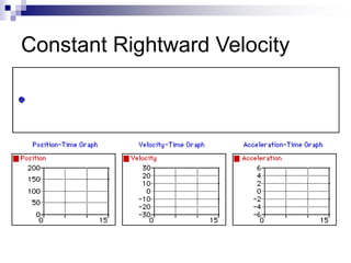
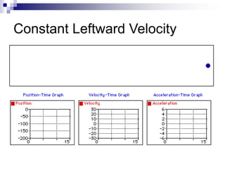
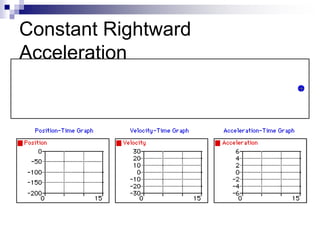
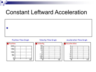
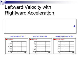
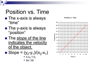
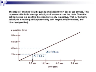
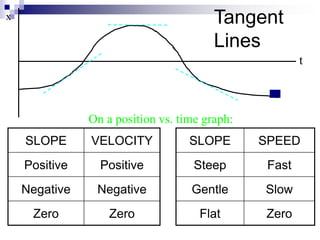
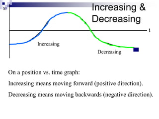
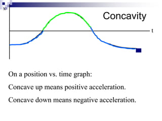
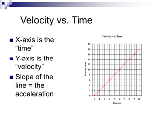
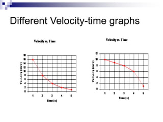
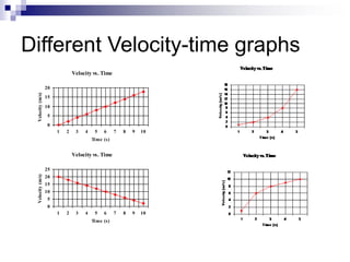
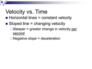
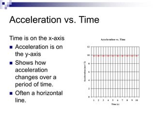
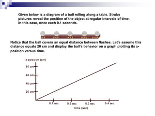
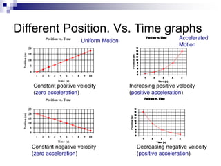
This document provides an overview of graphing motion in one dimension. It discusses position versus time graphs, velocity versus time graphs, and acceleration versus time graphs. Key points include: - The slope of a position-time graph represents velocity, and the slope of a velocity-time graph represents acceleration. - Straight lines on position-time graphs indicate uniform motion with constant velocity. 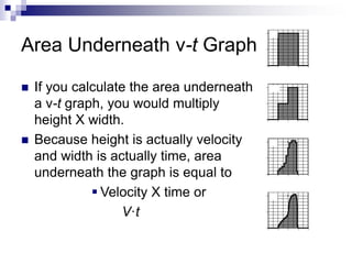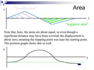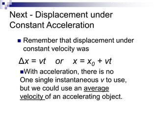- The area under a velocity-time graph represents displacement. 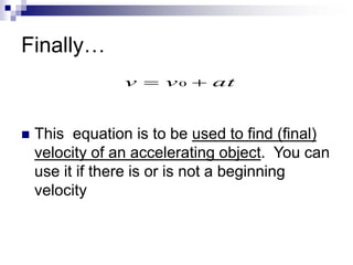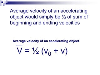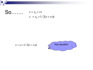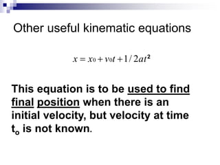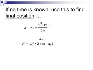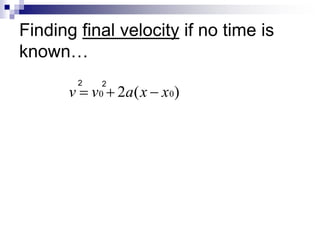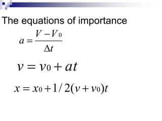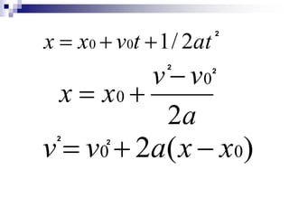- Kinematic equations allow calculations of variables like position, velocity, and acceleration given information about an object's motion under constant acceleration.

1. Motion 1D
CHAPTER 2
AP PHYSICS

2. Graphing Motion in One Dimension
 Interpret graphs of position versus time for
a moving object to determine the velocity
of the object
 Describe in words the information
presented in graphs and draw graphs from
descriptions of motion
 Write equations that describe the position
of an object moving at constant velocity

3. Parts of a
Graph
X-axis
Y-axis
All axes must be labeled with
appropriate units, and values.

4. Position vs. Time
 The x-axis is always
“time”
 The y-axis is always
“position”
 The slope of the line
indicates the velocity
of the object.
 Slope = (y2-y1)/(x2-x1)
 x-x0 / t-t0
 Δx / Δt
Position vs. Time
20
18
16
14
12
10
8
6
4
2
0
1 2 3 4 5 6 7 8 9 10
Time (s)
Position (m)

5. Uniform Motion
 Uniform motion is defined as equal
displacements occurring during
successive equal time periods
 Straight lines on position-time graphs
mean uniform motion.

6. Given below is a diagram of a ball rolling along a table. Strobe
pictures reveal the position of the object at regular intervals of time,
in this case, once each 0.1 seconds.
Notice that the ball covers an equal distance between flashes. Let's assume this
distance equals 20 cm and display the ball's behavior on a graph plotting its x-position
versus time.

7. The slope of this line would equal 20 cm divided by 0.1 sec or 200 cm/sec. This
represents the ball's average velocity as it moves across the table. Since the
ball is moving in a positive direction its velocity is positive. That is, the ball's
velocity is a vector quantity possessing both magnitude (200 cm/sec) and
direction (positive).

8. Steepness of slope on Position-
Time graph
Slope is related to velocity
Steep slope = higher
velocity
Shallow slope = less
velocity

9. Different Position. Vs. Time graphs
Position vs. Time
20
15
10
5
0
1 2 3 4 5 6 7 8 9 10
Time (s)
Position (m)
Position vs. Time
25
20
15
10
5
0
1 2 3 4 5 6 7 8 9 10
Time (s)
Position (m)
Constant positive velocity
(zero acceleration)
Constant negative velocity
(zero acceleration)
Increasing positive velocity
(positive acceleration)
Decreasing negative velocity
(positive acceleration)
Uniform Motion
Accelerated
Motion

10. X
t
A
B
C
A … Starts at home (origin) and goes forward slowly
B … Not moving (position remains constant as time
progresses)
C … Turns around and goes in the other direction quickly,
passing up home

11. During which intervals was he traveling in a positive direction?
During which intervals was he traveling in a negative direction?
During which interval was he resting in a negative location?
During which interval was he resting in a positive location?
During which two intervals did he travel at the same speed?
A) 0 to 2 sec B) 2 to 5 sec C) 5 to 6 sec D)6 to 7 sec E) 7 to 9 sec F)9 to 11 sec

12. Graphing w/
Acceleration
x
A … Start from rest south of home; increase speed gradually
B … Pass home; gradually slow to a stop (still moving north)
C … Turn around; gradually speed back up again heading south
D … Continue heading south; gradually slow to a stop near the
starting point
t
A
B C
D

13. Tangent
Lines
t
SLOPE VELOCITY
Positive Positive
Negative Negative
Zero Zero
SLOPE SPEED
Steep Fast
Gentle Slow
Flat Zero
x
On a position vs. time graph:

14. Increasing &
Decreasing
t
x
Increasing
Decreasing
On a position vs. time graph:
Increasing means moving forward (positive direction).
Decreasing means moving backwards (negative direction).

15. Concavity
t
x
On a position vs. time graph:
Concave up means positive acceleration.
Concave down means negative acceleration.

16. Special
Points
t
x
P
Q
R
Inflection Pt. P, R
S
Change of concavity,
change of acceleration
Peak or
Valley
Q
Turning point, change of
positive velocity to
negative
Time Axis
Intercept
P, S
Times when you are at
“home”, or at origin

17. Next - Graphing Velocity in One
Dimension
 Determine, from a graph of velocity versus
time, the velocity of an object at a specific
time
 Interpret a v-t graph to find the time at
which an object has a specific velocity
 Calculate the displacement of an object
from the area under a v-t graph

18. Velocity vs. Time
 X-axis is the
“time”
 Y-axis is the
“velocity”
 Slope of the
line = the
acceleration
Velocity vs. Time
20
18
16
14
12
10
8
6
4
2
0
1 2 3 4 5 6 7 8 9 10
Time (s)
Velcoity (m/s)

19. Different Velocity-time graphs

20. Different Velocity-time graphs
Velocity vs. Time
20
15
10
5
0
1 2 3 4 5 6 7 8 9 10
Time (s)
Velocity (m/s)
Velocity vs. Time
25
20
15
10
5
0
1 2 3 4 5 6 7 8 9 10
Time (s)
Velocity (m/s)

21. Velocity vs. Time
 Horizontal lines = constant velocity
 Sloped line = changing velocity
Steeper = greater change in velocity per
second
Negative slope = deceleration

22. Acceleration vs. Time
Time is on the x-axis
 Acceleration is on
the y-axis
 Shows how
acceleration
changes over a
period of time.
 Often a horizontal
line.
Acceleration vs. Time
12
10
8
6
4
2
0
1 2 3 4 5 6 7 8 9 10
Time (s)
Acceleration (m/s^2)

23. All 3 Graphs
t
x
v
t
a
t

24. Real life
Note how the v graph is pointy and the a graph skips. In real life,
the blue points would be smooth curves and the orange segments
would be connected. In our class, however, we’ll only deal with
constant acceleration.
a
t
v
t

25. Constant Rightward Velocity

26. Constant Leftward Velocity

27. Constant Rightward
Acceleration

28. Constant Leftward Acceleration

29. Leftward Velocity with
Rightward Acceleration

30. Graph Practice
Male all three graphs for the following scenario:
1. Newberry starts out north of home. At time zero he’s
driving a cement mixer south very fast at a constant speed.
2. He accidentally runs over an innocent moose crossing
the road, so he slows to a stop to check on the poor moose.
3. He pauses for a while until he determines the moose is
squashed flat and deader than a doornail.
4. Fleeing the scene of the crime, Newberry takes off again
in the same direction, speeding up quickly.
5. When his conscience gets the better of him, he slows,
turns around, and returns to the crash site.

31. Area Underneath v-t Graph
 If you calculate the area underneath
a v-t graph, you would multiply
height X width.
 Because height is actually velocity
and width is actually time, area
underneath the graph is equal to
 Velocity X time or
V·t

32.  Remember that Velocity = Δx
Δt
 Rearranging, we get Δx = velocity X Δt
 So….the area underneath a velocity-time
graph is equal to the displacement during
that time period.

33. Area v
t
“positive area”
“negative area”
Note that, here, the areas are about equal, so even though a
significant distance may have been covered, the displacement is
about zero, meaning the stopping point was near the starting point.
The position graph shows this as well.
t
x

34. Velocity vs. Time
 The area under a velocity time graph indicates
the displacement during that time period.
 Remember that the slope of the line indicates
the acceleration.
 The smaller the time units the more
“instantaneous” is the acceleration at that
particular time.
 If velocity is not uniform, or is changing, the
acceleration will be changing, and cannot be
determined “for an instant”, so you can only find
average acceleration

35. Acceleration
 Determine from the curves on a velocity-time
graph both the constant and
instantaneous acceleration
 Determine the sign of acceleration using a
v-t graph and a motion diagram
 Calculate the velocity and the
displacement of an object undergoing
constant acceleration

36. Acceleration
 Like speed or velocity,
acceleration is a rate
of change, defined as
the rate of change of
velocity
 Average Acceleration
= change in velocity
V V
t
a



0
Elapsed time Units of acceleration?

37. Rearrangement of the equation
V V
t
a



0
at  v  v0
v0  at  v
v  v0  at

38. Finally…
v  v0  at
 This equation is to be used to find (final)
velocity of an accelerating object. You can
use it if there is or is not a beginning
velocity

39. Next - Displacement under
Constant Acceleration
 Remember that displacement under
constant velocity was
Δx = vt or x = x0 + vt
With acceleration, there is no
One single instantaneous v to use,
but we could use an average
velocity of an accelerating object.

40. Average velocity of an accelerating
object would simply be ½ of sum of
beginning and ending velocities
Average velocity of an accelerating object
V = ½ (v0 + v)

41. So…….
x  x 
vt
x x v v t
0 1/ 2( 0)
0
  
x  x0 1/ 2(v  v0)t Key equation

42. Other useful kinematic equations
x  x0  v0t 1/ 2at 2
This equation is to be used to find
final position when there is an
initial velocity, but velocity at time
to is not known.

43. If no time is known, use this to find
final position….
v v
a
x x
2
0
0

 
2
2
v2 = vo
aka
2 + 2 a (x – xo )

44. Finding final velocity if no time is
known…
2 2
v  v0  2a(x  x0)

45. The equations of importance
V V
t
a



0
v  v0  at
x  x0 1/ 2(v  v0)t

46. x  x0  v0t 1/ 2at
v v
a
x x
2
2
0
0

 
2
2
2
v  v0 2
 2a(x  x0)

47. Practical Application
Velocity/Position/Time equations
 Calculation of arrival times/schedules of aircraft/trains
(including vectors)
 GPS technology (arrival time of signal/distance to
satellite)
 Military targeting/delivery
 Calculation of Mass movement (glaciers/faults)
 Ultrasound (speed of sound) (babies/concrete/metals)
Sonar (Sound Navigation and Ranging)
 Auto accident reconstruction
 Explosives (rate of burn/expansion rates/timing with det.
cord)