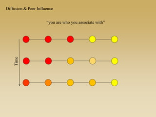
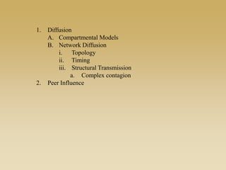
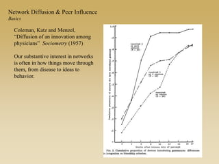
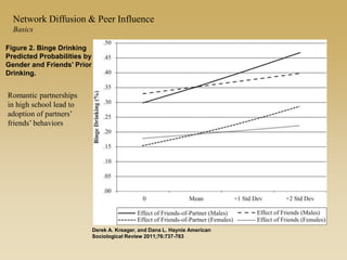
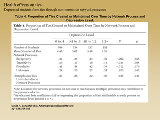
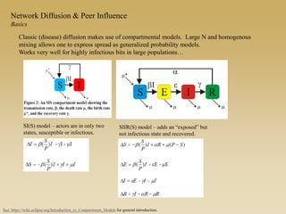
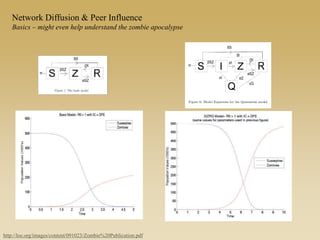
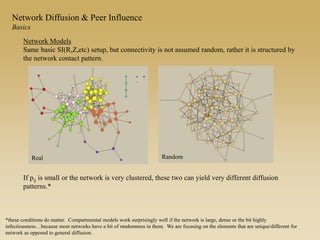
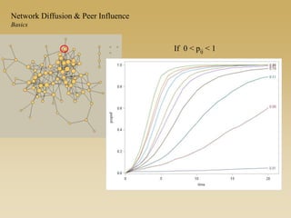
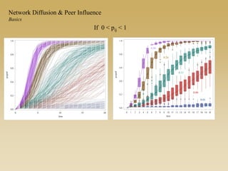
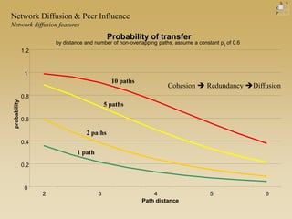
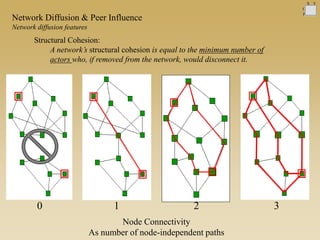
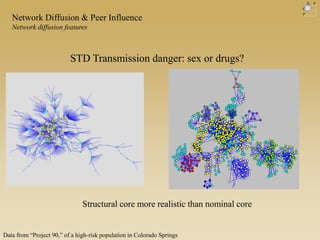
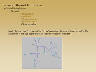
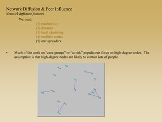
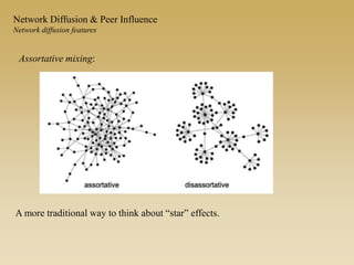
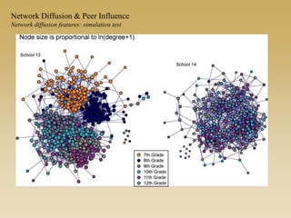
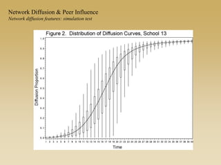
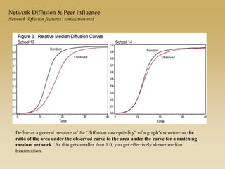
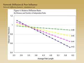
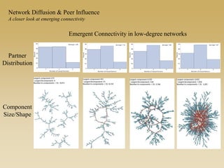
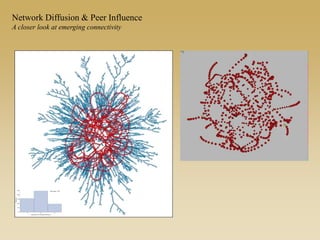
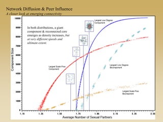
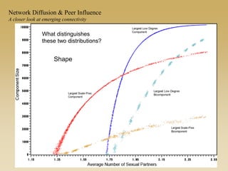
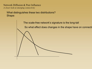
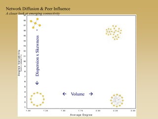
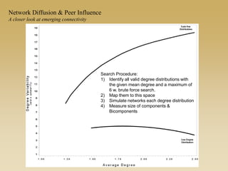
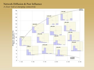
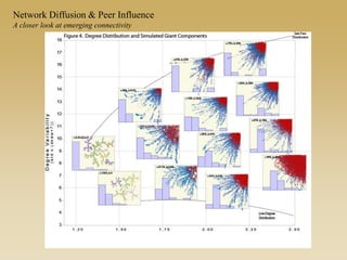
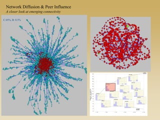
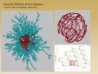
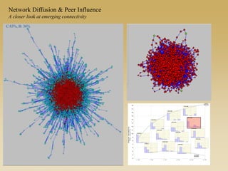
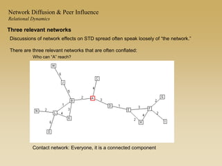
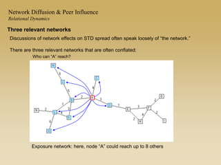
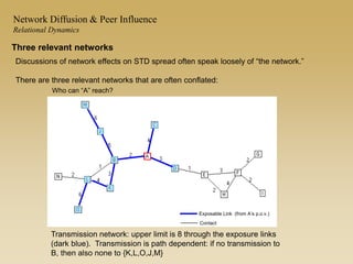
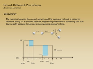
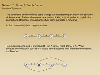
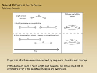
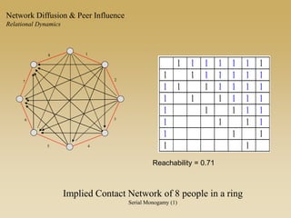
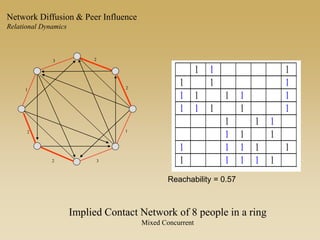
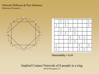
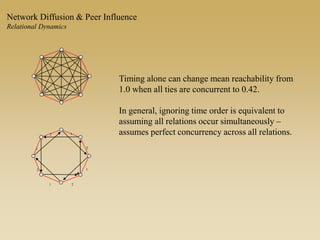
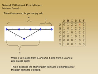
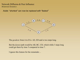
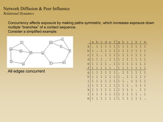
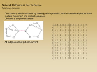
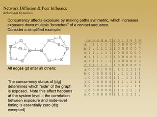
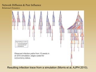
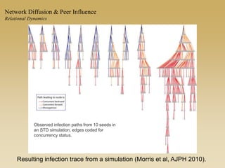
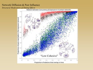
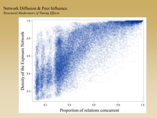
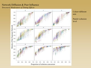
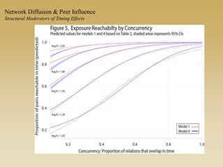
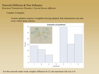
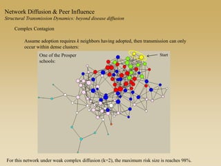
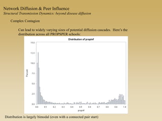
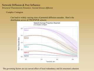
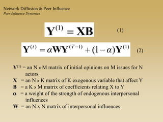
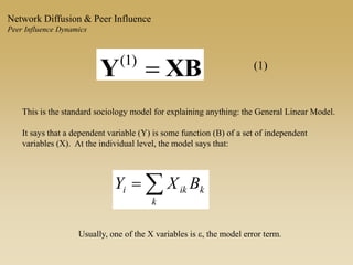
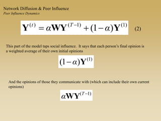
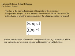
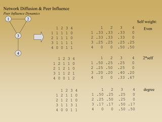
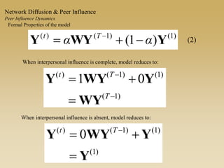
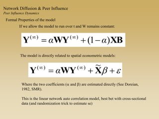
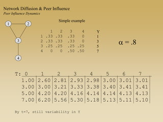
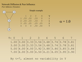
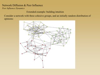
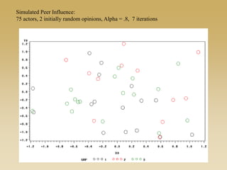
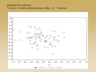
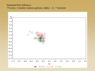
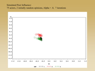
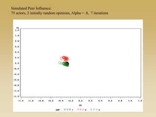
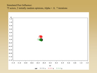
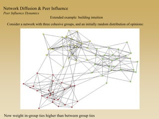
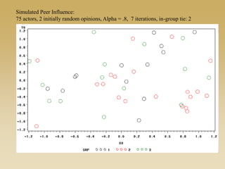
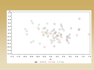
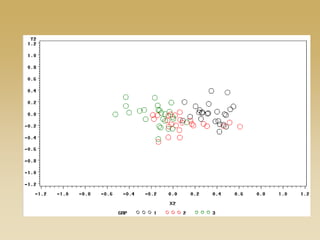
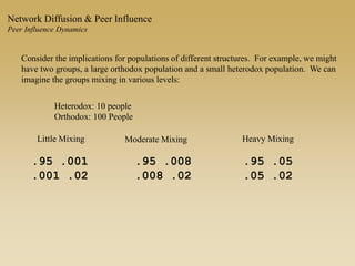
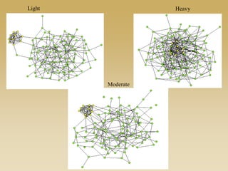
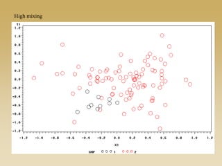
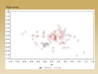
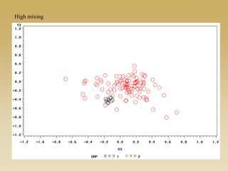
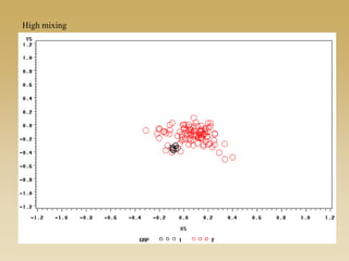
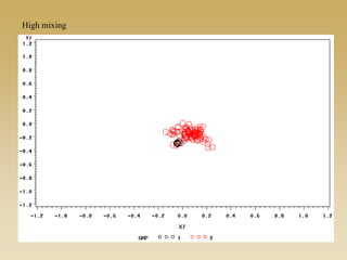
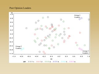
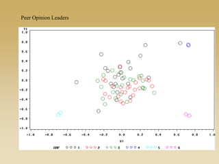
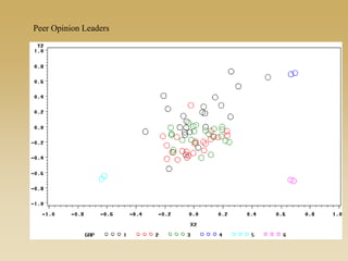
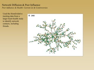
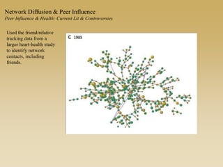
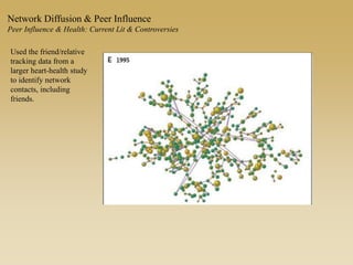
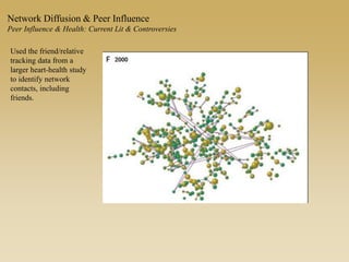
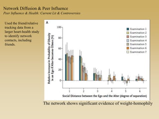
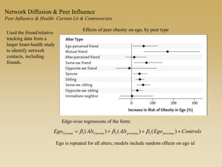
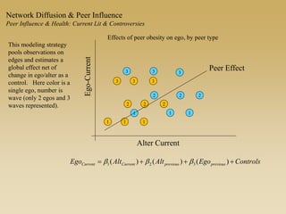
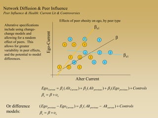
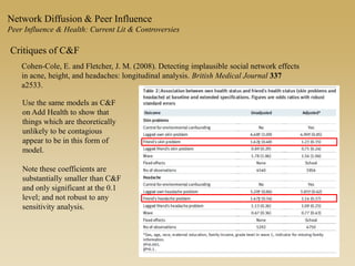
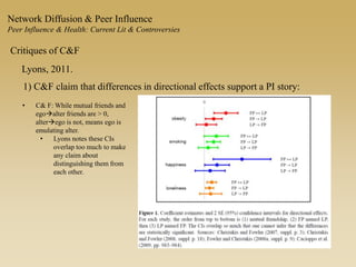
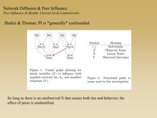
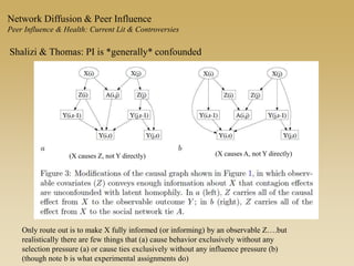
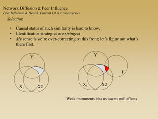
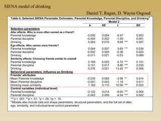
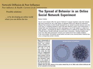
This document discusses diffusion and peer influence through networks. It begins by defining diffusion and compartment models used to model disease spread. It then discusses how network structure, including topology, timing of connections, and clustering, can impact diffusion compared to random mixing. Key network features that influence diffusion speed and reach include distance between actors, number of alternate paths, presence of highly connected "star" nodes, and assortative mixing. The document concludes by exploring how different degree distributions in emergent low-density networks can impact the formation of large connected components.
How to conduct a social network analysis: A tool for empowering teams and wor...Jeromy Anglim
Slides and details available at: http://jeromyanglim.blogspot.com/2009/10/how-to-conduct-social-network-analysis.html
A talk on using social network analysis as a team development tool.
How to conduct a social network analysis: A tool for empowering teams and wor...Jeromy Anglim
Slides and details available at: http://jeromyanglim.blogspot.com/2009/10/how-to-conduct-social-network-analysis.html
A talk on using social network analysis as a team development tool.
Inferring Peer Centrality in Socially-Informed Peer-to-Peer SystemsNicolas Kourtellis
Social applications implemented on a peer-to-peer (P2P) architecture mine the social graph of their users for improved performance in search, recommendations, resource
sharing and others. In such applications, the social graph that connects their users is distributed on the peer-to-peer system: the traversal of the social graph translates to a socially-informed routing in the peer-to-peer layer.
In this work we introduce the model of a projection graph that is the result of mapping a social graph onto a peer-to-peer network. We analytically formulate the relation between metrics in the social graph and in the projection graph. We focus on three such graph metrics: degree centrality, node betweenness centrality, and edge betweenness centrality. We evaluate experimentally the feasibility of estimating these metrics in the projection graph from the metrics of the social graph. Our experiments on real networks show that when mapping communities of 50-150 users on a peer, there is an optimal organization of the projection graph with respect to degree and node betweenness centrality. In this range, the association between the properties of the social graph and the projection graph is the highest, and thus the properties of the (dynamic) projection graph can be inferred from
the properties of the (slower changing) social graph. We discuss the applicability of our findings to aspects of peer-to-peer systems such as data dissemination, social search, peer vulnerability, and data placement and caching.
Inferring Peer Centrality in Socially-Informed Peer-to-Peer Systems. Nicolas Kourtellis and Adriana Iamnitchi. In Proceedings of 11th IEEE International Conference on Peer-to-Peer Computing (P2P'11), Kyoto, Japan, Aug 2011
COMMUNICATIONS OF THE ACM November 2004Vol. 47, No. 11 15.docxmonicafrancis71118
COMMUNICATIONS OF THE ACM November 2004/Vol. 47, No. 11 15
N
etworks are hot. The
Internet has made it pos-
sible to observe and mea-
sure linkages
representing relationships of
all kinds. We now recognize
networks everywhere: air
traffic, banking, chemical
bonds, data communications,
ecosystems, finite element
grids, fractals, interstate
highways, journal citations,
material structures, nervous
systems, oil pipelines, orga-
nizational networks, power
grids, social structures, trans-
portation, voice communica-
tion, water supply, Web
URLs, and more.
Several fields are collabo-
rating on the development of
network theory, measurement,
and mapping: mathematics
(graph theory), sociology (net-
works of influence and communi-
cation), computing (Internet), and
business (organizational net-
works). This convergence has pro-
duced useful results for risk
assessment and reduction in com-
plex infrastructure networks,
attacking and defending networks,
protecting against network con-
nectivity failures, operating busi-
nesses, spreading epidemics
(pathogens as well as computer
viruses), and spreading innova-
tion. Here, I will survey the fun-
damental laws of networks that
enable these results.
Defining a Network
A network is usually defined as a
set of nodes and links. The nodes
represent entities such as persons,
machines, molecules, documents,
or businesses; the links represent
relationships between pairs of
entities. A link can be directed
(one-way relationship) or undi-
rected (mutual relationship). A
hop is a transition from one node
to another across a single link
separating them. A path is a series
of hops. Networks are very gen-
eral: they can represent any kind
of relation among entities.
Some common network
topologies (interconnection pat-
terns) have their own names:
clique or island (a connected sub-
network that may be isolated
from other cliques), hierarchical
network (tree structured), hub-
and-spoke network (a special
node, the hub, connected directly
to every other node), and multi-
hub network (several hubs con-
nected directly to many nodes).
Some network topologies are
planned, such as the electric grid,
the interstate highway system, or
Network Laws
M
IC
H
A
EL
S
LO
A
N
Peter J. Denning
Many networks, physical and social, are complex and scale-invariant.
This has important implications from the spread of epidemics and
innovations to protection from attack.
The Profession of IT
16 November 2004/Vol. 47, No. 11 COMMUNICATIONS OF THE ACM
the air traffic system; others are
unplanned. In his seminal papers
about the Internet, Paul Baran
proposed that a planned, distrib-
uted network would be more
resilient to failures than a hub-
and-spoke network.
A host of physical systems eas-
ily fit a network model. Perhaps
less obvious is that human social
networks also fit the model. The
individuals of an organization are
linked by their relationships—
who emails whom, who seeks
advice from whom, or who influ-
ences w.
Using Social Network Analysis for Assessing Team Capacity and CollaborationJocelyne Helbling
Example applications for using Social Network Analysis (SNA) to assess research capacity and collaboration within a large. multi-institutional research team.
Daniel Martin Katz (Illinois Tech - Chicago Kent) & Michael Bommarito (Computational Legal Studies.com) Present Network Analysis and Law: Introductory Tutorial @ Jurix 2011 (Vienna)
These days considering expansion of networks, dissemination of information has become one of significant cases for researchers. In social networks in addition to social structures and people effectiveness on each other, Profit increase of sales, publishing a news or rumor, spread or diffusion of an idea can be mentioned. In social societies, people affect each other and with an individual’s membership, his friends
may join that group as well. In publishing a piece of news, independent of its nature there are different ways to expand it. Since information isn’t always suitable and positive, this article is trying to introduce the immunization mechanism against this information. The meaning of immunization is a kind of Slow Publishing of such information in network. Therefor it has been tried in this article to slow down the
publishing of information or even stop them. With comparison of presented methods for immunization and also presenting rate delay parameter, the immunization of methods were evaluated and we identified the most effective immunization method. Among existing methods for immunization and recommended methods, recommended methods also have an effective role in preventing spread of malicious rumor.
Social network plays a fundamental role as a medium for the spread of INFLUENCE among its members. As part of this research, estimates for influence between individuals were presented.
Comprehensive Analysis on the Vulnerability and Efficiency of P2P Networks un...ijp2p
Peer-to-peer systems are the networks consisting of a group of nodes possible to be as wide as the Internet.
These networks are required of evaluation mechanisms and distributed control and configurations, so each
peer (node) will be able to communicate with other peers. P2P networks actually act as the specific
transportation systems created to provide some services such as searching, large-scale storage, context
sharing, and supervisioning. Changes in configuration, possibly the resultant effects of faults and failures
or of the natural nodes behavior, are one of the most important features in P2P networks. Resilience to
faults and failures, and also an appropriate dealing with threats and attacks, are the main requirements of
today’s most communication systems and networks. Thus, since P2P networks can be individually used as
an infrastructure and an alternative for many other communication networks, they have to be more
reliable, accessible, and resilient to the faults, failures and attacks compared to the client/server approach.
In this work on progress, we present a detailed study on the behavior of various P2P networks toward
faults and failures, and focus on fault-tolerance subject. We consider two different static failure scenarios:
a) a random strategy in which nodes or edges of the network will be removed with an equal probability and
without any knowledge of the network’s infrastructure, b) a targeted strategy that uses some information
about the nodes, and in which the nodes with the highest degree have the most priority to be attacked. By
static faults, we mean a situation where the nodes or components encounter some faults before the network
starts to work or through its operation, and will remain faulty to the end of the work session. Our goal is to
introduce various measures to analyzing P2P networks evaluating their vulnerability rate. The presented
criteria can be used for evaluating the reliability and vulnerability of P2P networks toward both random
and targeted failures. There is no limit to the number and types of failures, the presented measures are able
to be used for different types of failures and even a wide range of networks.
Comprehensive Analysis on the Vulnerability and Efficiency of P2P Networks un...ijp2p
Peer-to-peer systems are the networks consisting of a group of nodes possible to be as wide as the Internet.
These networks are required of evaluation mechanisms and distributed control and configurations, so each
peer (node) will be able to communicate with other peers. P2P networks actually act as the specific
transportation systems created to provide some services such as searching, large-scale storage, context
sharing, and supervisioning. Changes in configuration, possibly the resultant effects of faults and failures
or of the natural nodes behavior, are one of the most important features in P2P networks. Resilience to
faults and failures, and also an appropriate dealing with threats and attacks, are the main requirements of
today’s most communication systems and networks. Thus, since P2P networks can be individually used as
an infrastructure and an alternative for many other communication networks, they have to be more
reliable, accessible, and resilient to the faults, failures and attacks compared to the client/server approach.
In this work on progress, we present a detailed study on the behavior of various P2P networks toward
faults and failures, and focus on fault-tolerance subject. We consider two different static failure scenarios:
a) a random strategy in which nodes or edges of the network will be removed with an equal probability and
without any knowledge of the network’s infrastructure, b) a targeted strategy that uses some information
about the nodes, and in which the nodes with the highest degree have the most priority to be attacked. By
static faults, we mean a situation where the nodes or components encounter some faults before the network
starts to work or through its operation, and will remain faulty to the end of the work session. Our goal is to
introduce various measures to analyzing P2P networks evaluating their vulnerability rate. The presented
criteria can be used for evaluating the reliability and vulnerability of P2P networks toward both random
and targeted failures. There is no limit to the number and types of failures, the presented measures are able
to be used for different types of failures and even a wide range of networks
Similar to 09 Diffusion Models & Peer Influence (20)
Seminar of U.V. Spectroscopy by SAMIR PANDASAMIR PANDA
Spectroscopy is a branch of science dealing the study of interaction of electromagnetic radiation with matter.
Ultraviolet-visible spectroscopy refers to absorption spectroscopy or reflect spectroscopy in the UV-VIS spectral region.
Ultraviolet-visible spectroscopy is an analytical method that can measure the amount of light received by the analyte.
What is greenhouse gasses and how many gasses are there to affect the Earth.moosaasad1975
What are greenhouse gasses how they affect the earth and its environment what is the future of the environment and earth how the weather and the climate effects.
Nutraceutical market, scope and growth: Herbal drug technologyLokesh Patil
As consumer awareness of health and wellness rises, the nutraceutical market—which includes goods like functional meals, drinks, and dietary supplements that provide health advantages beyond basic nutrition—is growing significantly. As healthcare expenses rise, the population ages, and people want natural and preventative health solutions more and more, this industry is increasing quickly. Further driving market expansion are product formulation innovations and the use of cutting-edge technology for customized nutrition. With its worldwide reach, the nutraceutical industry is expected to keep growing and provide significant chances for research and investment in a number of categories, including vitamins, minerals, probiotics, and herbal supplements.
This presentation explores a brief idea about the structural and functional attributes of nucleotides, the structure and function of genetic materials along with the impact of UV rays and pH upon them.
Richard's entangled aventures in wonderlandRichard Gill
Since the loophole-free Bell experiments of 2020 and the Nobel prizes in physics of 2022, critics of Bell's work have retreated to the fortress of super-determinism. Now, super-determinism is a derogatory word - it just means "determinism". Palmer, Hance and Hossenfelder argue that quantum mechanics and determinism are not incompatible, using a sophisticated mathematical construction based on a subtle thinning of allowed states and measurements in quantum mechanics, such that what is left appears to make Bell's argument fail, without altering the empirical predictions of quantum mechanics. I think however that it is a smoke screen, and the slogan "lost in math" comes to my mind. I will discuss some other recent disproofs of Bell's theorem using the language of causality based on causal graphs. Causal thinking is also central to law and justice. I will mention surprising connections to my work on serial killer nurse cases, in particular the Dutch case of Lucia de Berk and the current UK case of Lucy Letby.
Earliest Galaxies in the JADES Origins Field: Luminosity Function and Cosmic ...Sérgio Sacani
We characterize the earliest galaxy population in the JADES Origins Field (JOF), the deepest
imaging field observed with JWST. We make use of the ancillary Hubble optical images (5 filters
spanning 0.4−0.9µm) and novel JWST images with 14 filters spanning 0.8−5µm, including 7 mediumband filters, and reaching total exposure times of up to 46 hours per filter. We combine all our data
at > 2.3µm to construct an ultradeep image, reaching as deep as ≈ 31.4 AB mag in the stack and
30.3-31.0 AB mag (5σ, r = 0.1” circular aperture) in individual filters. We measure photometric
redshifts and use robust selection criteria to identify a sample of eight galaxy candidates at redshifts
z = 11.5 − 15. These objects show compact half-light radii of R1/2 ∼ 50 − 200pc, stellar masses of
M⋆ ∼ 107−108M⊙, and star-formation rates of SFR ∼ 0.1−1 M⊙ yr−1
. Our search finds no candidates
at 15 < z < 20, placing upper limits at these redshifts. We develop a forward modeling approach to
infer the properties of the evolving luminosity function without binning in redshift or luminosity that
marginalizes over the photometric redshift uncertainty of our candidate galaxies and incorporates the
impact of non-detections. We find a z = 12 luminosity function in good agreement with prior results,
and that the luminosity function normalization and UV luminosity density decline by a factor of ∼ 2.5
from z = 12 to z = 14. We discuss the possible implications of our results in the context of theoretical
models for evolution of the dark matter halo mass function.
Slide 1: Title Slide
Extrachromosomal Inheritance
Slide 2: Introduction to Extrachromosomal Inheritance
Definition: Extrachromosomal inheritance refers to the transmission of genetic material that is not found within the nucleus.
Key Components: Involves genes located in mitochondria, chloroplasts, and plasmids.
Slide 3: Mitochondrial Inheritance
Mitochondria: Organelles responsible for energy production.
Mitochondrial DNA (mtDNA): Circular DNA molecule found in mitochondria.
Inheritance Pattern: Maternally inherited, meaning it is passed from mothers to all their offspring.
Diseases: Examples include Leber’s hereditary optic neuropathy (LHON) and mitochondrial myopathy.
Slide 4: Chloroplast Inheritance
Chloroplasts: Organelles responsible for photosynthesis in plants.
Chloroplast DNA (cpDNA): Circular DNA molecule found in chloroplasts.
Inheritance Pattern: Often maternally inherited in most plants, but can vary in some species.
Examples: Variegation in plants, where leaf color patterns are determined by chloroplast DNA.
Slide 5: Plasmid Inheritance
Plasmids: Small, circular DNA molecules found in bacteria and some eukaryotes.
Features: Can carry antibiotic resistance genes and can be transferred between cells through processes like conjugation.
Significance: Important in biotechnology for gene cloning and genetic engineering.
Slide 6: Mechanisms of Extrachromosomal Inheritance
Non-Mendelian Patterns: Do not follow Mendel’s laws of inheritance.
Cytoplasmic Segregation: During cell division, organelles like mitochondria and chloroplasts are randomly distributed to daughter cells.
Heteroplasmy: Presence of more than one type of organellar genome within a cell, leading to variation in expression.
Slide 7: Examples of Extrachromosomal Inheritance
Four O’clock Plant (Mirabilis jalapa): Shows variegated leaves due to different cpDNA in leaf cells.
Petite Mutants in Yeast: Result from mutations in mitochondrial DNA affecting respiration.
Slide 8: Importance of Extrachromosomal Inheritance
Evolution: Provides insight into the evolution of eukaryotic cells.
Medicine: Understanding mitochondrial inheritance helps in diagnosing and treating mitochondrial diseases.
Agriculture: Chloroplast inheritance can be used in plant breeding and genetic modification.
Slide 9: Recent Research and Advances
Gene Editing: Techniques like CRISPR-Cas9 are being used to edit mitochondrial and chloroplast DNA.
Therapies: Development of mitochondrial replacement therapy (MRT) for preventing mitochondrial diseases.
Slide 10: Conclusion
Summary: Extrachromosomal inheritance involves the transmission of genetic material outside the nucleus and plays a crucial role in genetics, medicine, and biotechnology.
Future Directions: Continued research and technological advancements hold promise for new treatments and applications.
Slide 11: Questions and Discussion
Invite Audience: Open the floor for any questions or further discussion on the topic.
2. “you are who you associate with”
Time
Diffusion & Peer Influence
3. 1. Diffusion
A. Compartmental Models
B. Network Diffusion
i. Topology
ii. Timing
iii. Structural Transmission
a. Complex contagion
2. Peer Influence
4. Coleman, Katz and Menzel,
“Diffusion of an innovation among
physicians” Sociometry (1957)
Our substantive interest in networks
is often in how things move through
them, from disease to ideas to
behavior.
Network Diffusion & Peer Influence
Basics
5. Figure 2. Binge Drinking
Predicted Probabilities by
Gender and Friends’ Prior
Drinking.
Derek A. Kreager, and Dana L. Haynie American
Sociological Review 2011;76:737-763
Romantic partnerships
in high school lead to
adoption of partners’
friends’ behaviors
Network Diffusion & Peer Influence
Basics
6. Table 4. Proportion of Ties Created or Maintained Over Time by Network Process and
Depression Level.
David R. Schaefer et al. American Sociological Review
2011;76:764-785
Health effects on ties
Depressed students form ties through non-normative network processes
7. Network Diffusion & Peer Influence
Basics
Classic (disease) diffusion makes use of compartmental models. Large N and homogenous
mixing allows one to express spread as generalized probability models.
Works very well for highly infectious bits in large populations…
SI(S) model – actors are in only two
states, susceptible or infectious.
See: https://wiki.eclipse.org/Introduction_to_Compartment_Models for general introduction.
SIIR(S) model – adds an “exposed” but
not infectious state and recovered.
8. Network Diffusion & Peer Influence
Basics – might even help understand the zombie apocalypse
http://loe.org/images/content/091023/Zombie%20Publication.pdf
9. Network Diffusion & Peer Influence
Basics
Network Models
Same basic SI(R,Z,etc) setup, but connectivity is not assumed random, rather it is structured by
the network contact pattern.
If pij is small or the network is very clustered, these two can yield very different diffusion
patterns.*
Real Random
*these conditions do matter. Compartmental models work surprisingly well if the network is large, dense or the bit highly
infectiousness…because most networks have a bit of randomness in them. We are focusing on the elements that are unique/different for
network as opposed to general diffusion.
12. In addition to* the dyadic probability that one actor passes something to another
(pij), two factors affect flow through a network:
Topology
- the shape, or form, of the network
- Example: one actor cannot pass information to another unless they are
either directly or indirectly connected
Time
- the timing of contact matters
- Example: an actor cannot pass information he has not receive yet
*This is a big conditional! – lots of work on how the dyadic transmission rate may differ across
populations.
Key Question: What features of a network contribute most to diffusion potential?
Network Diffusion & Peer Influence
Network diffusion features
Use simulation tools to explore the relative effects of structural
connectivity features
13. • A network has to be connected for a bit to pass over it
• If transmission is uncertain, the longer the distance the lower the likelihood of spread.
0
0.2
0.4
2 3 4 5 6
Path distance
probability
Distance and diffusion (p(transfer)=pij
dist
Here pij of 0.6
Network Diffusion & Peer Influence
Network diffusion features
We need:
(1) reachability
(2) distance
(3) local clustering
(4) multiple routes
(5) star spreaders
14. • Local clustering turns flow “in” on a potential transmission tree
Arcs: 11
Largest component: 12,
Clustering: 0
Arcs: 11
Largest component: 8,
Clustering: 0.205
We need:
(1) reachability
(2) distance
(3) local clustering
(4) multiple routes
(5) star spreaders
Network Diffusion & Peer Influence
Network diffusion features
15. • The more alternate routes one has for transmission, the more likely flow should be.
• Operationalize alternate routes with structural cohesion
We need:
(1) reachability
(2) distance
(3) local clustering
(4) multiple routes
(5) star spreaders
Network Diffusion & Peer Influence
Network diffusion features
16. Probability of transfer
by distance and number of non-overlapping paths, assume a constant pij of 0.6
0
0.2
0.4
0.6
0.8
1
1.2
2 3 4 5 6
Path distance
probability
1 path
C
P
X Y
10 paths
5 paths
2 paths
Cohesion Redundancy Diffusion
Network Diffusion & Peer Influence
Network diffusion features
17. 0 1 2 3
Node Connectivity
As number of node-independent paths
C
P
X Y
Structural Cohesion:
A network’s structural cohesion is equal to the minimum number of
actors who, if removed from the network, would disconnect it.
Network Diffusion & Peer Influence
Network diffusion features
18. STD Transmission danger: sex or drugs?
Structural core more realistic than nominal core
C
P
X Y
Data from “Project 90,” of a high-risk population in Colorado Springs
Network Diffusion & Peer Influence
Network diffusion features
19. • Much of the work on “core groups” or “at risk” populations focus on high-degree nodes. The
assumption is that high-degree nodes are likely to contact lots of people.
We need:
(1) reachability
(2) distance
(3) local clustering
(4) multiple routes
(5) star spreaders
Network Diffusion & Peer Influence
Network diffusion features
20. • Much of the work on “core groups” or “at risk” populations focus on high-degree nodes. The
assumption is that high-degree nodes are likely to contact lots of people.
We need:
(1) reachability
(2) distance
(3) local clustering
(4) multiple routes
(5) star spreaders
Network Diffusion & Peer Influence
Network diffusion features
21. Network Diffusion & Peer Influence
Network diffusion features
Assortative mixing:
A more traditional way to think about “star” effects.
22. • Simulation study: How do these different features compare over a collection of observed nets?
• For each network trial:
• Fix dyadic transmission probability
• Randomly select a node as seed
• Trace the diffusion path across the network
• Measure speed & extent of spread
• Model extent of spread by structural characteristics
• First run: Add Health:
• simple diffusion process
• dyadic probability set to 0.08
• 500 trials in each network.
• Then expand to :
• Different assumptions of dyadic transmission probability
• Different data set (Facebook)
• Complex diffusion models
Network Diffusion & Peer Influence
Network diffusion features: simulation test
25. Define as a general measure of the “diffusion susceptibility” of a graph’s structure as the
ratio of the area under the observed curve to the area under the curve for a matching
random network. As this gets smaller than 1.0, you get effectively slower median
transmission.
Network Diffusion & Peer Influence
Network diffusion features: simulation test
26. Figure 4. Relative Diffusion Ratio
By Distance and Number of Independent Paths
0.4
0.6
0.8
1
1.2
2.3 2.8 3.3 3.8 4.3 4.8 5.3 5.8 6.3
Average Path Length
Observed/Random
k=2
k=4
k=6
k=8
Figure 4. Relative Diffusion Ratio
By Distance and Number of Independent Paths
0.4
0.6
0.8
1
1.2
2.3 2.8 3.3 3.8 4.3 4.8 5.3 5.8 6.3
Average Path Length
Observed/Random
k=2
k=4
k=6
k=8
Network Diffusion & Peer Influence
Network diffusion features: simulation test
27. Traditional “core group” models have a local-vision understanding of risk: those
with lots of ties (high degree) are the focus for intervention and actions.
•In the short time-windows necessary for STD transfer, low-degree networks are
the relevant features for transmission. What sorts of networks emerge when
average degree (in the short run) is held to small numbers?
•How does the shape of the degree distribution matter? If activity is homogeneous
do we get fundamentally different networks than if it is very heterogeneous?
Network Diffusion & Peer Influence
A closer look at emerging connectivity
30. In both distributions, a giant
component & reconnected core
emerges as density increases, but
at very different speeds and
ultimate extent.
Network Diffusion & Peer Influence
A closer look at emerging connectivity
31. What distinguishes
these two distributions?
Shape
Network Diffusion & Peer Influence
A closer look at emerging connectivity
32. What distinguishes these two distributions?
Shape:
The scale-free network’s signature is the long-tail
So what effect does changes in the shape have on connectiv
Network Diffusion & Peer Influence
A closer look at emerging connectivity
34. Search Procedure:
1) Identify all valid degree distributions with
the given mean degree and a maximum of
6 w. brute force search.
2) Map them to this space
3) Simulate networks each degree distribution
4) Measure size of components &
Bicomponents
Network Diffusion & Peer Influence
A closer look at emerging connectivity
35. Based on work supported by R21-HD072810 (NICHD, Moody PI), R01 HD068523-01 (NICHD, Moody PI), R01 DA012831-05 (NIDA Morris, Martina PI),
Network Diffusion & Peer Influence
A closer look at emerging connectivity
36. Based on work supported by R21-HD072810 (NICHD, Moody PI), R01 HD068523-01 (NICHD, Moody PI), R01 DA012831-05 (NIDA Morris, Martina PI),
Network Diffusion & Peer Influence
A closer look at emerging connectivity
37. C:45%, B: 8.5%
Based on work supported by R21-HD072810 (NICHD, Moody PI), R01 HD068523-01 (NICHD, Moody PI), R01 DA012831-05 (NIDA Morris, Martina PI),
Network Diffusion & Peer Influence
A closer look at emerging connectivity
38. C:45%, B: 8.5%
Based on work supported by R21-HD072810 (NICHD, Moody PI), R01 HD068523-01 (NICHD, Moody PI), R01 DA012831-05 (NIDA Morris, Martina PI),
Network Diffusion & Peer Influence
A closer look at emerging connectivity
39. C:83%, B: 36%
Based on work supported by R21-HD072810 (NICHD, Moody PI), R01 HD068523-01 (NICHD, Moody PI), R01 DA012831-05 (NIDA Morris, Martina PI),
Network Diffusion & Peer Influence
A closer look at emerging connectivity
40. Based on work supported by R21-HD072810 (NICHD, Moody PI), R01 HD068523-01 (NICHD, Moody PI), R01 DA012831-05 (NIDA Morris, Martina PI),
C:99%, B: 86%
Network Diffusion & Peer Influence
A closer look at emerging connectivity
41. Largest Component
(at least 1 path)
Largest Bicomponent
(at least 2 paths)
Based on work supported by R21-HD072810 (NICHD, Moody PI), R01 HD068523-01 (NICHD, Moody PI), R01 DA012831-05 (NIDA Morris, Martina PI),
Network Diffusion & Peer Influence
A closer look at emerging connectivity
42. In addition to* the dyadic probability that one actor passes something to another
(pij), two factors affect flow through a network:
Topology
- the shape, or form, of the network
- Example: one actor cannot pass information to another unless they are
either directly or indirectly connected
Time
- the timing of contact matters
- Example: an actor cannot pass information he has not receive yet
*This is a big conditional! – lots of work on how the dyadic transmission rate may differ across
populations.
Key Question: What features of a network contribute most to diffusion potential?
Network Diffusion & Peer Influence
Relational Dynamics
Use simulation tools to explore the relative effects of structural
connectivity features
43. Three relevant networks
Discussions of network effects on STD spread often speak loosely of “the network.”
There are three relevant networks that are often conflated:
1) The contact network. The set of pairs of people connected by sexual contact. G(V,E).
2) The exposure network. A subset of the edges in the contact network where timing
makes it possible for one person to pass infection to another.
3) The transmission network. The subset of the exposure network where disease is actually
passed. In most cases this is a tree layered on (2) and rooted on a source/seed node.
Network Diffusion & Peer Influence
Relational Dynamics
44. Contact network: Everyone, it is a connected component
Who can “A” reach?
Network Diffusion & Peer Influence
Relational Dynamics
Discussions of network effects on STD spread often speak loosely of “the network.”
There are three relevant networks that are often conflated:
Three relevant networks
45. Exposure network: here, node “A” could reach up to 8 others
Who can “A” reach?
Network Diffusion & Peer Influence
Relational Dynamics
Discussions of network effects on STD spread often speak loosely of “the network.”
There are three relevant networks that are often conflated:
Three relevant networks
46. Transmission network: upper limit is 8 through the exposure links
(dark blue). Transmission is path dependent: if no transmission to
B, then also none to {K,L,O,J,M}
Who can “A” reach?
Exposable Link (from A’s p.o.v.)
Contact
Network Diffusion & Peer Influence
Relational Dynamics
Discussions of network effects on STD spread often speak loosely of “the network.”
There are three relevant networks that are often conflated:
Three relevant networks
47. The mapping between the contact network and the exposure network is based on
relational timing. In a dynamic network, edge timing determines if something can flow
down a path because things can only be passed forward in time.
Definitions:
Two edges are adjacent if they share a node.
A path is a sequence of adjacent edges (E1, E2, …Ed).
A time-ordered path is a sequence of adjacent edges where, for each pair of
edges in the sequence, the start time Si is less than or equal to Ej S(E1) <
E(E2)
Adjacent edges are concurrent if they share a node and have start and end
dates that overlap. This occurs if:
S(E2) < E(E1)
Concurrency
Network Diffusion & Peer Influence
Relational Dynamics
48. A B C
D
time 1 2 3 4 5 6 7 8 9 10
AB
BC
CE
E
CD
2 - 71 - 3
S(ab) E(ab)
S(bc)
E(bc)
S(ce) E(ce)
The mapping between the contact network and the exposure network is based on
relational timing. In a dynamic network, edge timing determines if something can flow
down a path because things can only be passed forward in time.
Concurrency
Network Diffusion & Peer Influence
Relational Dynamics
49. The constraints of time-ordered paths change our understanding of the system structure
of the network. Paths make a network a system: linking actors together through indirect
connections. Relational timing changes how paths cumulate in networks.
Indirect connectivity is no longer transitive:
A B C D1 - 2 3 - 4 1 - 2
Here A can reach C, and C and reach D. But A cannot reach D (nor D A). Why?
Because any infection A passes to C would have happened after the relation between C
and D ended.
A B C D1 - 2 3 - 4 1 - 2
Network Diffusion & Peer Influence
Relational Dynamics
50. Edge time structures are characterized by sequence, duration and overlap.
Paths between i and j, have length and duration, but these need not be
symmetric even if the constituent edges are symmetric.
Network Diffusion & Peer Influence
Relational Dynamics
54. Implied Contact Network of 8 people in a ring
Serial Monogamy (3)
1 1 1
1 1 1
1 1 1
1 1 1
1 1 1
1 1 1
1 1 1
1 1 1
1
2
1
1
2
1
2
2
Reachability = 0.43
Network Diffusion & Peer Influence
Relational Dynamics
55. 1
2
1
1
2
1
2
2
Timing alone can change mean reachability from
1.0 when all ties are concurrent to 0.42.
In general, ignoring time order is equivalent to
assuming all relations occur simultaneously –
assumes perfect concurrency across all relations.
Network Diffusion & Peer Influence
Relational Dynamics
56. A B C D E F
A 0 1 2 2 4 1
B 1 0 1 2 3 2
C 0 1 0 1 2 2
D 0 0 1 0 1 1
E 0 0 0 1 0 2
F 1 0 0 1 0 0
While a is 2 steps from d, and d is 1 step from e, a and e
are 4 steps apart.
This is because the shorter path from a to e emerges after
the path from d to e ended.
4
2
1
Path distances no longer simply add
Network Diffusion & Peer Influence
Relational Dynamics
57. A
B C
D
3 - 4
E
The geodesic from A to D is AE, ED and is two steps long.
But the fastest path would be AB, BC, CD, which while 3 steps long
could get there by time 5 compared to time 7.
I ignore this feature for the remainder…
Aside: “shortest” can now be replaced with “fastest”
Network Diffusion & Peer Influence
Relational Dynamics
58. Concurrency affects exposure by making paths symmetric, which increases exposure down
multiple “branches” of a contact sequence.
Consider a simplified example:
All edges concurrent
a b c d e f g h i j k l m
a . 1 1 1 1 1 1 1 1 1 1 1 1
b 1 . 1 1 1 1 1 1 1 1 1 1 1
c 1 1 . 1 1 1 1 1 1 1 1 1 1
d 1 1 1 . 1 1 1 1 1 1 1 1 1
e 1 1 1 1 . 1 1 1 1 1 1 1 1
f 1 1 1 1 1 . 1 1 1 1 1 1 1
g 1 1 1 1 1 1 . 1 1 1 1 1 1
h 1 1 1 1 1 1 1 . 1 1 1 1 1
i 1 1 1 1 1 1 1 1 . 1 1 1 1
j 1 1 1 1 1 1 1 1 1 . 1 1 1
k 1 1 1 1 1 1 1 1 1 1 . 1 1
l 1 1 1 1 1 1 1 1 1 1 1 . 1
m 1 1 1 1 1 1 1 1 1 1 1 1 .
Network Diffusion & Peer Influence
Relational Dynamics
59. All edges except gd concurrent
a b c d e f g h i j k l m
a . 1 1 1 1 1 1 1 1 1 1 1 1
b 1 . 1 1 1 1 1 1 1 1 1 1 1
c 1 1 . 1 1 1 1 1 1 1 1 1 1
d 1 1 1 . 1 1 1 1 1 1 1 1 1
e 1 1 1 1 . 1 1 1 1 1 1 1 1
f 1 1 1 1 1 . 1 1 1 1 1 1 1
g 0 0 0 1 0 0 . 1 1 1 1 1 1
h 0 0 0 1 0 0 1 . 1 1 1 1 1
i 0 0 0 1 0 0 1 1 . 1 1 1 1
j 0 0 0 1 0 0 1 1 1 . 1 1 1
k 0 0 0 1 0 0 1 1 1 1 . 1 1
l 0 0 0 1 0 0 1 1 1 1 1 . 1
m 0 0 0 1 0 0 1 1 1 1 1 1 .
Concurrency affects exposure by making paths symmetric, which increases exposure down
multiple “branches” of a contact sequence.
Consider a simplified example:
Network Diffusion & Peer Influence
Relational Dynamics
60. Concurrency affects exposure by making paths symmetric, which increases
exposure down multiple “branches” of a contact sequence.
Consider a simplified example:
All edges gd after all others:
a b c d e f g h i j k l m
a . 1 1 1 1 1 1 0 0 0 0 0 0
b 1 . 1 1 1 1 1 0 0 0 0 0 0
c 1 1 . 1 1 1 1 0 0 0 0 0 0
d 1 1 1 . 1 1 1 0 0 0 0 0 0
e 1 1 1 1 . 1 1 0 0 0 0 0 0
f 1 1 1 1 1 . 1 0 0 0 0 0 0
g 0 0 0 1 0 0 . 1 1 1 1 1 1
h 0 0 0 0 0 0 1 . 1 1 1 1 1
i 0 0 0 0 0 0 1 1 . 1 1 1 1
j 0 0 0 0 0 0 1 1 1 . 1 1 1
k 0 0 0 0 0 0 1 1 1 1 . 1 1
l 0 0 0 0 0 0 1 1 1 1 1 . 1
m 0 0 0 0 0 0 1 1 1 1 1 1 .
The concurrency status of {dg}
determines which “side” of the graph
is exposed. Note this effect happens
at the system level – the correlation
between exposure and node-level
timing is essentially zero (d/g
excepted)
Network Diffusion & Peer Influence
Relational Dynamics
61. Resulting infection trace from a simulation (Morris et al, AJPH 2010).
Observed infection paths from 10 seeds in
an STD simulation, edges coded for
concurrency status.
Network Diffusion & Peer Influence
Relational Dynamics
62. Resulting infection trace from a simulation (Morris et al, AJPH 2010).
Network Diffusion & Peer Influence
Relational Dynamics
Observed infection paths from 10 seeds in
an STD simulation, edges coded for
concurrency status.
63. Timing constrains potential diffusion paths in networks, since bits can flow through edges that have
ended.
This means that:
• Structural paths are not equivalent to the diffusion-relevant path set.
• Network distances don’t build on each other.
• Weakly connected components overlap without diffusion reaching across sets.
• Small changes in edge timing can have dramatic effects on overall diffusion
• Diffusion potential is maximized when edges are concurrent and minimized when they are
“inter-woven” to limit reachability.
Combined, this means that many of our standard path-based network measures will be incorrect on
dynamic graphs.
Network Diffusion & Peer Influence
Relational Dynamics
64. Measures
Dependent variable: Reachability in the exposure graph. This is the proportion of
pairs in the network that are reachable in time.
Exposure Graph Density
Network Diffusion & Peer Influence
Structural Moderators of Timing Effects
67. Measures: Independent variables
Features of the topology. Of key interest is the level of structural cohesion.
Average connectivity
Network Diffusion & Peer Influence
Structural Moderators of Timing Effects
74. 1. Concurrency has a necessarily positive effect on potential diffusion
exposure
1. This implies that we should see greater transmission given greater
concurrency
2. This works by creating “multiple routes” in the exposure path
structure
2. Structural cohesion captures multiple routes in the contact graph
1. Higher levels of cohesion increase exposure by directly increasing
the underlying transmission substrate
3. There is a negative interaction between cohesion and concurrency: as
cohesion increases, the relative returns to concurrency decrease.
1. But this comes at the cost of a higher base-level of exposure.
Network Diffusion & Peer Influence
Structural Moderators of Timing Effects
75. Network Diffusion & Peer Influence
Structural Transmission Dynamics: beyond disease diffusion
Complex Contagion
Thus far we have focused on a “simple” dyadic diffusion parameter, pij, where the
probability of passing/receiving the bit is purely dependent on discordant status of
the dyad, sometimes called the “independent cascade model” (), which suggests a
monotonic relation between the number of times you are exposed through peers.
High exposure could be due to repeated interaction with one person or weak
interaction with many, effectively equating:
Alternative models exist. Under “complex contagion” for example, the likelihood
that I accept the bit that flows through the network depends on the proportion of my
peers that have the bit.
76. Network Diffusion & Peer Influence
Structural Transmission Dynamics: beyond disease diffusion
1
1
2
3
Complex Contagion
Assume adoption requires k neighbors having adopted, then transmission can only
occur within dense clusters:
77. Network Diffusion & Peer Influence
Structural Transmission Dynamics: beyond disease diffusion
Complex Contagion
Assume adoption requires k neighbors having adopted, then transmission can only
occur within dense clusters:
Assume pij=1, k=2, starting nodes in yellow
78. Network Diffusion & Peer Influence
Structural Transmission Dynamics: beyond disease diffusion
Complex Contagion
Assume adoption requires k neighbors having adopted, then transmission can only
occur within dense clusters:
For this network under weak complex diffusion (k=2), the maximum risk size is 8.
79. Network Diffusion & Peer Influence
Structural Transmission Dynamics: beyond disease diffusion
Complex Contagion
Assume adoption requires k neighbors having adopted, then transmission can only
occur within dense clusters:
For this network under weak complex diffusion (k=2), the maximum risk size is reaches 98%.
One of the Prosper
schools:
Start
80. Network Diffusion & Peer Influence
Structural Transmission Dynamics: beyond disease diffusion
Complex Contagion
Can lead to widely varying sizes of potential diffusion cascades. Here’s the
distribution across all PROPSPER schools:
Distribution is largely bimodal (even with a connected pair start)
81. Network Diffusion & Peer Influence
Structural Transmission Dynamics: beyond disease diffusion
Complex Contagion
Can lead to widely varying sizes of potential diffusion cascades. Here’s the
distribution across all PROPSPER schools:
The governing factors are (a) curved effect of local redundancy and (b) structural cohesion
Network Average Proportion Reached
k=2 complex contagion
MeanCascadeSize
Coh=0.3
Coh=1.2
Coh=2.2
Coh=3.2
Coh=4.1
82. Network Diffusion & Peer Influence
Structural Transmission Dynamics: beyond disease diffusion
Complex Contagion
Does get used for real health
work:
Here , authors assume a CC
process, seeded with observed
depressive cases, turn that into
a Markov model and ask what
parameters would maximize fit
from simulated to observed.
83. Network Diffusion & Peer Influence
Structural Transmission Dynamics: beyond disease diffusion
Complex diffusion is just the most well studied of the options that combine
transmission with some pairwise positional feature. This is a wide-open
area for future research.
The basic idea is that transmission is increased/decreased if there is some
third structural property that the susceptible & infected pair share.
This leads us into the general problem of peer influence models…when do
peers change each other’s behaviors?
84. Background:
• Long standing research interest in how our relations shape our attitudes
and behaviors.
• Most often assumed mechanism is that people (through conversation or
similar) change each others beliefs/opinions, which changes behavior.
This implies that position in a communication network should be related
to attitudes.
• Alternatives:
• Modeling behavior: ego copies behavior of alter to gain respect,
esteem, etc.
• Distinction: Ego tries to be different from (some) alter to gain
respect, esteem, etc.
• Access: Ego wants to do Y, but can only do so because alter provides
access (say, being old enough to buy cigarettes).
Network Diffusion & Peer Influence
Peer Influence Dynamics
85. Background:
• Early work was ego-centric – people informed on their peers
•Seems to have inflated PI effects by ~50% or so…either through projection of
ego behavior onto peers or selective interaction (what alters do with ego may be
different than what alter does all the time).
•Then to cross sectional associations based on alter self-reports
•Better, but still likely conflates selection with influence
•Next to dynamic models:
•Ego Behavior(t) ~ f(ego behavior(t-1) + alter behavior (t-1) + controls
•Much better; still debate on (a) correct estimation functions, (b) unobserved
selection features that confound causal inference.
•Development of Actor-oriented models (SIENA)
Network Diffusion & Peer Influence
Peer Influence Dynamics
86. Background:
•Finally: Experimental manipulation of peer exposure
•“Gold standard” for isolation of peer effects
•Likely strongly underestimates effects (as measure intent to treat, not take-
up of treatment, since people may not care about relations that can be
manipulated).
b(Peer(y)): Ego Inform < Alter Inform < Cross Sectional < Dynamic < Experimental. Still often
find peer effects, but my sense is that we’ve (strongly) over-corrected at this point.
Network Diffusion & Peer Influence
Peer Influence Dynamics
87. Freidkin’s Structural Theory of Social Influence :
Two-part model:
Beliefs are a function of two sources:
a) Individual characteristics
•Gender, Age, Race, Education, Etc. Standard sociology
b) Interpersonal influences
•Actors negotiate with others
Network Diffusion & Peer Influence
Peer Influence Dynamics
88. XBY )1( (1)
)1()1()(
)1( YWYY αα Tt
(2)
Y(1) = an N x M matrix of initial opinions on M issues for N
actors
X = an N x K matrix of K exogenous variable that affect Y
B = a K x M matrix of coefficients relating X to Y
a = a weight of the strength of endogenous interpersonal
influences
W = an N x N matrix of interpersonal influences
Network Diffusion & Peer Influence
Peer Influence Dynamics
89. XBY )1( (1)
This is the standard sociology model for explaining anything: the General Linear Model.
It says that a dependent variable (Y) is some function (B) of a set of independent
variables (X). At the individual level, the model says that:
k
kiki BXY
Usually, one of the X variables is e, the model error term.
Network Diffusion & Peer Influence
Peer Influence Dynamics
90. )1()1()(
)1( YWYY αα Tt
(2)
This part of the model taps social influence. It says that each person’s final opinion is
a weighted average of their own initial opinions
)1(
)1( Yα
And the opinions of those they communicate with (which can include their own current
opinions)
)1( T
αWY
Network Diffusion & Peer Influence
Peer Influence Dynamics
91. The key to the peer influence part of the model is W, a matrix of
interpersonal weights. W is a function of the communication structure of the
network, and is usually a transformation of the adjacency matrix. In general:
j
ij
ij
w
w
1
10
Various specifications of the model change the value of wii, the extent to which
one weighs their own current opinion and the relative weight of alters.
Network Diffusion & Peer Influence
Peer Influence Dynamics
93. )1()1()(
)1( YWYY αα Tt
Formal Properties of the model
When interpersonal influence is complete, model reduces to:
)1(
)1()1()(
01
T
Tt
WY
YWYY
When interpersonal influence is absent, model reduces to:
)1(
)1()1()(
0
Y
YWYY
Tt
(2)
Network Diffusion & Peer Influence
Peer Influence Dynamics
94. Formal Properties of the model
The model is directly related to spatial econometric models:
If we allow the model to run over t and W remains constant:
XBWYY )1()()(
αα
eb
XWYY
~)()(
α
Where the two coefficients (a and b) are estimated directly (See Doreian,
1982, SMR).
This is the linear network auto correlation model, best bet with cross-sectional
data (and randomization trick to estimate se)
Network Diffusion & Peer Influence
Peer Influence Dynamics
97. Extended example: building intuition
Consider a network with three cohesive groups, and an initially random distribution of
opinions:
Network Diffusion & Peer Influence
Peer Influence Dynamics
106. Extended example: building intuition
Consider a network with three cohesive groups, and an initially random distribution of opinions:
Now weight in-group ties higher than between group ties
Network Diffusion & Peer Influence
Peer Influence Dynamics
113. Consider the implications for populations of different structures. For example, we might
have two groups, a large orthodox population and a small heterodox population. We can
imagine the groups mixing in various levels:
Little Mixing Moderate Mixing Heavy Mixing
.95 .05
.05 .02
.95 .008
.008 .02
.95 .001
.001 .02
Heterodox: 10 people
Orthodox: 100 People
Network Diffusion & Peer Influence
Peer Influence Dynamics
133. In an unbalanced situation (small group vs large group) the extent of contact
can easily overwhelm the small group. Applications of this idea are evident
in:
•Missionary work (Must be certain to send missionaries out into the
world with strong in-group contacts)
•Overcoming deviant culture (I.e. youth gangs vs. adults)
•This is also the mechanism behind why most youth peer influence
is a *good* thing – most youth are well behavior and civic
minded…so are exerting positive influences on their peers.
Network Diffusion & Peer Influence
Peer Influence Dynamics
134. Friedkin (1998) generalizes the model so that alpha varies across people.
(1) simply changing a to a vector (A), which then changes each person’s
opinion directly
(2) by linking the self weight (wii) to alpha.
)1()1()(
)( YAIAWYY Tt
Were A is a diagonal matrix of endogenous weights, with 0 < aii < 1. A further
restriction on the model sets wii = 1-aii
This leads to a great deal more flexibility in the theory, and some interesting
insights. Consider the case of group opinion leaders with unchanging opinions
(I.e. many people have high aii, while a few have low):
Network Diffusion & Peer Influence
Peer Influence Dynamics
141. Further extensions of the model might:
• Time dependent a: people likely value other’s opinions more early than later in a
decision context
• Interact a with XB: people’s self weights are a function of their behaviors &
attributes
• Make W dependent on structure of the network (weight transitive ties greater
than intransitive ties, for example)
• Time dependent W: The network of contacts does not remain constant, but is
dynamic, meaning that influence likely moves unevenly through the network
• And others likely abound….
Network Diffusion & Peer Influence
Peer Influence Dynamics
142. There are two common ways to test for peer associations through networks.
The first estimates the parameters (a and b) of the network autocorrelation model directly,
the second transforms the network into a dyadic model, predicting similarity among
actors.
eb
XWYY
~)()(
α
Peer influence model:
Network Diffusion & Peer Influence
Peer Influence Dynamics
This is the linear network autocorrelation model, and as specified, the
model makes strong assumptions about equilibrium opinion and static
relations.
Some variants on this also expand e to include alternative
autocorrelation in the error structure.
143. There are two common ways to test for peer associations through networks.
The first estimates the parameters (a and b) of the network autocorrelation model directly,
the second transforms the network into a dyadic model, predicting similarity among
actors.
eb
XWYY
~)()(
α
Peer influence model:
Network Diffusion & Peer Influence
Peer Influence Dynamics
Note that since WY is a a simple vector -- weighted mean of friends Y -- which can be
constructed and added to your GLM model. That is, multiple Y by a W matrix, and run the
regression with WY as a new variable, and the regression coefficient is an estimate of a. This is
what Doriean calls the QAD estimate of peer influence.
It’s wrong, a will be biased, but it’s often not terribly wrong if most obvious selection factors are
built int0 X
144. An obvious problem with this specification is that cases are, by definition, not
independent, hence “network autocorrelation” terminology.
In practice, the QAD approach (perhaps combined with a GLS estimator)
results in empirical estimates that are “virtually indistinguishable” from MLE
(Doreian et al, 1984)
The proper way to estimate the peer equation is to use maximum likelihood
estimates, and Doreian gives the formulas for this in his paper, and Carter Butts
has implemented in in R with the LNAM procedure.
An alternative is to use non-parametric approaches, such as the Quadratic
Assignment Procedure, to estimate the effects.
Network Diffusion & Peer Influence
Peer Influence Dynamics
145. Peer influence through Dyad Models
Another way to get at peer influence is not through the level of Y, but by assessing the
similarity of connected peers. Recall the simulated example: peer influence is reflected in
how close points are to each other.
Network Diffusion & Peer Influence
Peer Influence Dynamics
146. Peer influence through Dyad Models
The model is now expressed at the dyad level as:
ij
k
kkijij eXbAbbY 10
Where Y is a matrix of similarities, A is an adjacency matrix, and Xk is a matrix of similarities
on attributes
Advantages include ease of specifying relation-specific similarity functions. You can add
different features of a relation by adjusting/adding “Aij” variables.
Disadvantage is that now in addition to network autocorrelation, you have repeated cases (on
both sides).
But these can be dealt with using non-parametric modeling & testing techniques (QAP, for
example). (which we will go over this afternoon)
Network Diffusion & Peer Influence
Peer Influence Dynamics
148. Used the friend/relative
tracking data from a
larger heart-health study
to identify network
contacts, including
friends.
Network Diffusion & Peer Influence
Peer Influence & Health: Current Lit & Controversies
149. Used the friend/relative
tracking data from a
larger heart-health study
to identify network
contacts, including
friends.
Network Diffusion & Peer Influence
Peer Influence & Health: Current Lit & Controversies
150. Used the friend/relative
tracking data from a
larger heart-health study
to identify network
contacts, including
friends.
Network Diffusion & Peer Influence
Peer Influence & Health: Current Lit & Controversies
151. Used the friend/relative
tracking data from a
larger heart-health study
to identify network
contacts, including
friends.
Network Diffusion & Peer Influence
Peer Influence & Health: Current Lit & Controversies
152. Used the friend/relative
tracking data from a
larger heart-health study
to identify network
contacts, including
friends.
Network Diffusion & Peer Influence
Peer Influence & Health: Current Lit & Controversies
153. Used the friend/relative
tracking data from a
larger heart-health study
to identify network
contacts, including
friends.
Network Diffusion & Peer Influence
Peer Influence & Health: Current Lit & Controversies
154. Used the friend/relative
tracking data from a
larger heart-health study
to identify network
contacts, including
friends.
Network Diffusion & Peer Influence
Peer Influence & Health: Current Lit & Controversies
155. The network shows significant evidence of weight-homophily
Used the friend/relative
tracking data from a
larger heart-health study
to identify network
contacts, including
friends.
Network Diffusion & Peer Influence
Peer Influence & Health: Current Lit & Controversies
156. Effects of peer obesity on ego, by peer type
Edge-wise regressions of the form:
ControlsEgoAltAltEgo previouspreviousCurrentCurrent )()()( 321 bbb
Ego is repeated for all alters; models include random effects on ego id
Used the friend/relative
tracking data from a
larger heart-health study
to identify network
contacts, including
friends.
Network Diffusion & Peer Influence
Peer Influence & Health: Current Lit & Controversies
157. This modeling strategy
pools observations on
edges and estimates a
global effect net of
change in ego/alter as a
control. Here color is a
single ego, number is
wave (only 2 egos and 3
waves represented).
Effects of peer obesity on ego, by peer type
ControlsEgoAltAltEgo previouspreviousCurrentCurrent )()()( 321 bbb
1
Ego-Current
Alter Current
1 1
2 2 2
3 3 3
1 1 1
2 2 2
3 3 3
Peer Effect
Network Diffusion & Peer Influence
Peer Influence & Health: Current Lit & Controversies
158. Alterative specifications
include using change-
change models and
allowing for a random
effect of peers. This
allows for greater
variability in peer effects,
and the potential to model
differences.
ee
currentpreviouseCurrentprevious ControlstAltAlEgoEgo
bb
b
)()(
1
Ego-Current
Alter Current
1 1
2 2 2
3 3 3
1 1 1
2 2 2
3 3 3
b
be1
be1
Effects of peer obesity on ego, by peer type
Network Diffusion & Peer Influence
Peer Influence & Health: Current Lit & Controversies
ee
previouspreviousCurrenteCurrent ControlsEgoAltAltEgo
bb
bbb
)()()( 32
Or difference
models:
159. Network Diffusion & Peer Influence
Peer Influence & Health: Current Lit & Controversies
Critiques of C&F
The C&F studies – of obesity, but also other work on the FHS data – turn on the validity of the
causal association.
All turn on some issue of model miss-specification, typically:
• Can’t truly distinguish a network effect from other sources of common influence
• “Selection” (“homophily”) or “Common influence” (“Shared environment”)
• The most strident work in this area (Salizi
• Statistical errors
• Misinterpretation of confidence intervals
• Poorly specified/estimated models
C&H do a nice job of laying out their responses here:
http://jhfowler.ucsd.edu/examining_dynamic_social_networks.pdf and here:
http://www.ncbi.nlm.nih.gov/pmc/articles/PMC2597062/
160. Network Diffusion & Peer Influence
Peer Influence & Health: Current Lit & Controversies
Critiques of C&F
Cohen-Cole, E. and Fletcher, J. M. (2008). Detecting implausible social network effects
in acne, height, and headaches: longitudinal analysis. British Medical Journal 337
a2533.
Use the same models as C&F
on Add Health to show that
things which are theoretically
unlikely to be contagious
appear to be in this form of
model.
Note these coefficients are
substantially smaller than C&F
and only significant at the 0.1
level; and not robust to any
sensitivity analysis.
161. Network Diffusion & Peer Influence
Peer Influence & Health: Current Lit & Controversies
Critiques of C&F
Lyons, 2011.
1) C&F claim that differences in directional effects support a PI story:
• C& F: While mutual friends and
egoalter friends are > 0,
alterego is not, means ego is
emulating alter.
• Lyons notes these CIs
overlap too much to make
any claim about
distinguishing them from
each other.
162. Network Diffusion & Peer Influence
Peer Influence & Health: Current Lit & Controversies
Critiques of C&F Lyons, 2011.
2) Insufficient controls for Homophily
• C& F: Use of alter’s lagged Y to control for homophily. Logic is that any feature
that selected us to be friends at t-1 would have had it’s effect then.
• Lyons notes that current and lagged have opposite signs, which seems
suspect, and anyway is an insufficient control. He’s likely right here…
3) Directionality cannot distinguish the source of association
• C& F: the ordering: mutual, egoalter, alterego suggests an “esteem” model,
where ego copies the behavior of alter.
• Lyons argues that we would expect the same logic from a simple “foci” of
similarity. I don’t find this argument convincing.
4) Random permutation tests cannot establish 3-degree rule
• C& F: Association between alters at 1, 2, 3 degrees of separation are higher than
we’d expect by chance, based on a permutation test.
• Lyons invalid if the data are incomplete, which they certainly are. I don’t
find this argument convincing…data are always incomplete…
163. Network Diffusion & Peer Influence
Peer Influence & Health: Current Lit & Controversies
Critiques of C&F Lyons, 2011.
5) The models are statistically inconsistent (if not incoherent)
• C& F: Use separate models for each type of tie, with random effects on ego.
• Lyons notes that these really should be treated as simultaneous equations,
with shared error structures and so forth. Doing so (a) leads to unidentified
models that must force the estimation of the peer effect to 0. That observed
^0 indicates something amiss.
• Strikes me as a bit down in the weeds and I’m not convinced here that he’s
critiquing them for what they are really doing (argues there are more
equations than data, which is patently not true).
164. Network Diffusion & Peer Influence
Peer Influence & Health: Current Lit & Controversies
Critiques of C&F Lyons, 2011.
My sense is that the strategy C&F took was not fundamentally misguided, but the model
specification is probably thin; certainly in the obesity paper – less so in some of the later papers
appearing after these debates.
Ideally you’d have a much better direct model for selection – perhaps even a separate two-stage
model (see the Siena module), but here there are very limited observational controls, which would
have been easy to add. In later specifications, they do add fixed effects for ego and still find similar
results.
Commenting on the debate on SocNET – and a related conclusion that only experiments could
provide valid inference – Tom Snijders says:
“The logical consequence of this is that we are stuck with imperfect methods. Lyons argues as
though only perfect methods are acceptable, and while applauding such lofty ideals I still believe
that we should accept imperfection, in life as in science. Progress is made by discussion and
improvement of imperfections, not by their eradication.”
For a full general discussion, see : https://www.lists.ufl.edu/cgi-bin/wa?A2=ind1106&L=SOCNET&P=R11428
165. Network Diffusion & Peer Influence
Peer Influence & Health: Current Lit & Controversies
Shalizi & Thomas: PI is *generally* confounded
So long as there is an unobserved X that causes both ties and behavior, the
effect of peers is unidentified.
166. Network Diffusion & Peer Influence
Peer Influence & Health: Current Lit & Controversies
Shalizi & Thomas: PI is *generally* confounded
Only route out is to make X fully informed (or informing) by an observable Z….but
realistically there are few things that (a) cause behavior exclusively without any
selection pressure (a) or cause ties exclusively without any influence pressure (b)
(though note b is what experimental assignments do)
(X causes Z, not Y directly) (X causes A, not Y directly)
167. Network Diffusion & Peer Influence
Peer Influence & Health: Current Lit & Controversies
Shalizi & Thomas: PI is *generally* confounded
Should be noted that this is true for *any* effect – there’s always the
potential that an unobserved latent variable is creating a spurious effect;
This sort of work argues that the only solution is to use experimental (or,
sometimes, propensity score style models)…but that’s simply not always
feasible practically.
We need to beware of making the best the enemy of the good enough…lest
we make no progress at all…
168. How to correct this problem?
•Essentially, this is an omitted variable problem, and my “solution” has
been to identify as many potentially relevant alternative variables as I can
find.
•The strongest possible correction is to use fixed-effects* models that
control for all non-varying individual covariates. These have their own
problems…
•Dual model for influence & selection.
•Two-stage model “Heckman” sorts of models
•Dynamic SAOM models
•Experiments
Network Diffusion & Peer Influence
Peer Influence & Health: Current Lit & Controversies
*“Adding fixed effects to dynamic panel models with many subjects and few repeat observations creates severe bias towards zero coefficients. This has
been demonstrated both analytically (Nickell 1981) and through simulations (Nerlove 1971) for OLS and other regression models and has been well-known
by social scientists, including economists, for a very long time. In fact, CCF even note that they do not add fixed effects to their logit regression model for
this reason, but they strangely assert that fixed effects are necessary in the OLS model.” Estimating Peer Effects on Health in Social Networks : A
Response to Cohen-Cole and Fletcher; Trogdon, Nonnemaker, Pais J.H. Fowler, PhD and N.A. Christakis, MD, PhD
169. • Causal status of such similarity is hard to know,
• Identification strategies are stringent
• My sense is we’re over-correcting on this front; let’s figure out what’s
there first.
Selection
Network Diffusion & Peer Influence
Peer Influence & Health: Current Lit & Controversies
Y
X1 X2
Weak instruments bias us toward null effects
Y
X1 X2
I
170. Possible solutions:
• Theory: Given what we know about how friendships form, is it reasonable
to assume a bi-directional cause? That is, work through the meeting,
socializing, etc. process and ask whether it makes sense that Y is a cause of
W. This will not convince a skeptical reader, but you should do it anyway.
• Models:
- Time Order. Necessary but not sufficient. We are on somewhat firmer
ground if W precedes Y in time, but the Shalizi & Thomas problem of
an as-yet-earlier joint confounder is still there.
- Simultaneous Models. Model both the friendship pattern and the
outcome of interest simultaneously. Best bet for direct estimation
•Sensitivity Analysis:
I think the most reasonable solution…take error potential seriously,
attempt to evaluate how big a problem it really is.
Network Diffusion & Peer Influence
Peer Influence & Health: Current Lit & Controversies
171. Table 4. Selected SIENA Parameter Estimates: Parental Knowledge, Parental Discipline, and Drinking
a
Model 2
b SE t SD
Selection parameters
Alter effects: Who is more often named as a friend?
Parental knowledge -0.002 0.004 -0.47 0.003
Parental discipline -0.004 0.002 -1.55 0.001
Drinking 0.083 0.010 8.69 *** 0.007
Ego effects: Who names more friends?
Parental knowledge 0.044 0.007 5.85 *** 0.039
Parental discipline -0.002 0.005 -0.36 0.023
Drinking -0.011 0.021 -0.53 0.089
Similarity effects: Choosing friends similar to oneself
Parental knowledge 0.169 0.025 6.70 *** 0.101
Parental discipline 0.151 0.017 8.86 *** 0.035
Drinking 0.276 0.021 13.45 *** 0.006
Behavioral parameters: Influence on Drinking
Friends' attributes
Mean Parental knowledge -0.230 0.065 -3.56 ** 0.014
Mean Parental discipline -0.051 0.043 -1.18 0.011
Drinking mean similarity 1.162 0.110 10.56 *** 0.023
Control variables (individual level)
Parental knowledge -0.122 0.014 -8.93 *** 0.004
Parental discipline -0.043 0.009 -4.54 *** 0.002
***p < .001. **p < .01. *p < .05. †p < .10.
a
Models also include rate and shape parameters, structural parameters, and the full set of alter,
ego, similarity, and individual-level control parameters
SIENA model of drinking
Daniel T. Ragan, D. Wayne Osgood
172. Possible solutions:
•Sensitivity Analysis:
I think the most
reasonable solution…take
error potential seriously,
attempt to evaluate how
big a problem it really is.
Network Diffusion & Peer Influence
Peer Influence & Health: Current Lit & Controversies
173. Possible solutions:
•Sensitivity Analysis:
I think the most reasonable solution…take error potential seriously, attempt to evaluate
how big a problem it really is.
Network Diffusion & Peer Influence
Peer Influence & Health: Current Lit & Controversies
Sociological Methods & Research 2000
174. Experimental designs may
alleviate this problem
Exogenously decide peers via natural
experiment…
Possible solutions:
Network Diffusion & Peer Influence
Peer Influence & Health: Current Lit & Controversies
175. … or by developing an online world
where you can define the ties
Possible solutions:
Network Diffusion & Peer Influence
Peer Influence & Health: Current Lit & Controversies