Download as PDF, PPTX

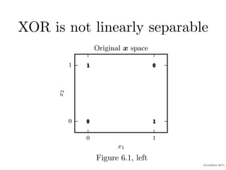


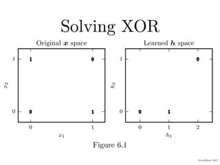


This document provides an overview of deep feedforward networks. It begins with an example of using a network to solve the XOR problem. It then discusses gradient-based learning and backpropagation. Hidden units with rectified linear activations are commonly used. Deeper networks can more efficiently represent functions and generalize better than shallow networks. Architecture design considerations include width, depth, and number of hidden layers. Backpropagation efficiently computes gradients using the chain rule and dynamic programming.