Downloaded 10 times
![IBS Statistics Year 1 Dr. Ning DING [email_address] I007, Friday & Monday](https://image.slidesharecdn.com/001-100914100422-phpapp01/85/001-1-320.jpg)
![IBS Statistics Year 1 Dr. Ning DING [email_address] I007, Friday & Monday](https://image.slidesharecdn.com/001-100914100422-phpapp01/75/001-1-2048.jpg)
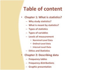
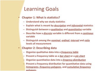
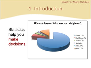
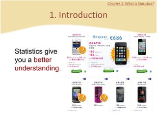
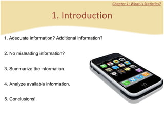
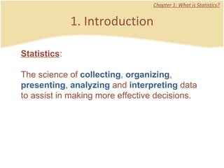
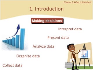
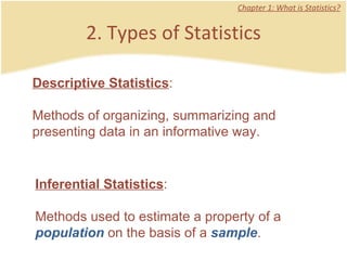
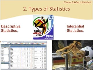
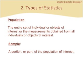
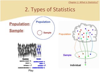
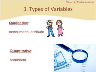
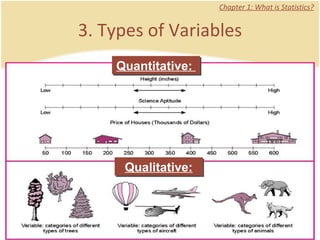
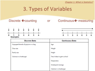
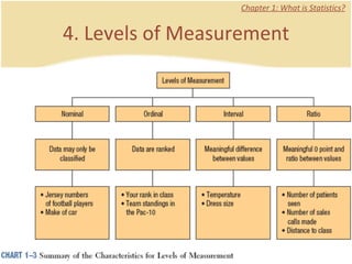
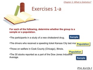
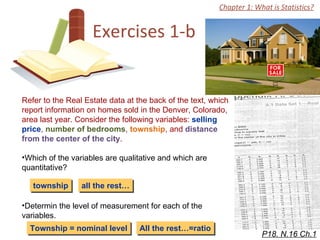
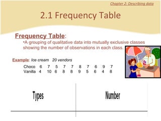
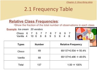
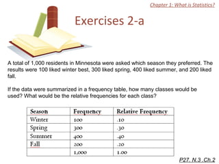
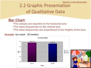
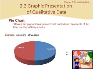
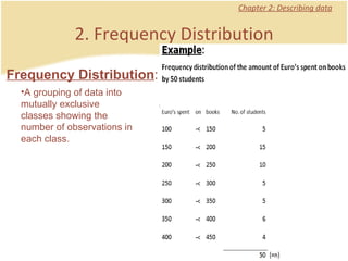
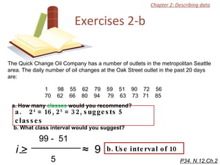
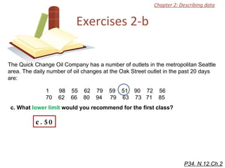
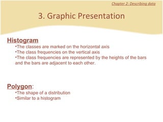
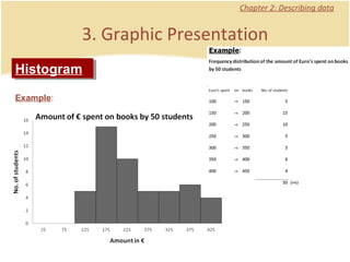
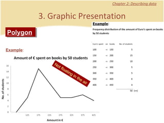
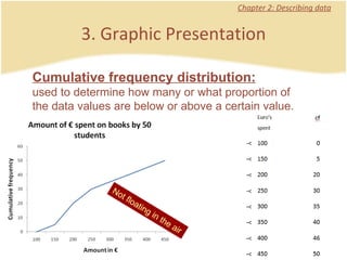
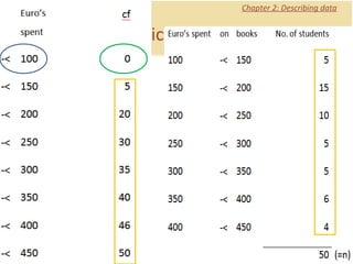
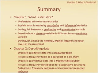
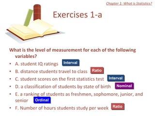
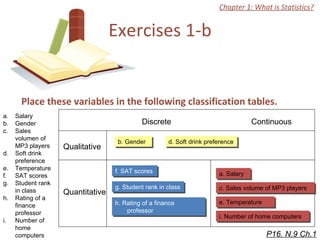
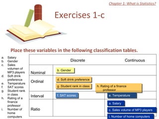
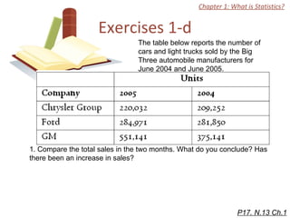

The document discusses introductory statistics concepts including descriptive statistics, inferential statistics, types of variables, levels of measurement, frequency tables, histograms, and other methods for organizing and presenting data. Chapter 1 covers what statistics is, types of statistics, variables, and levels of measurement. Chapter 2 discusses describing data through frequency tables, bar charts, histograms, and other graphs. The learning goals are to understand descriptive vs inferential statistics and distinguish between different statistical concepts.