Corso Pat Jgrasshorton 2008 10 17

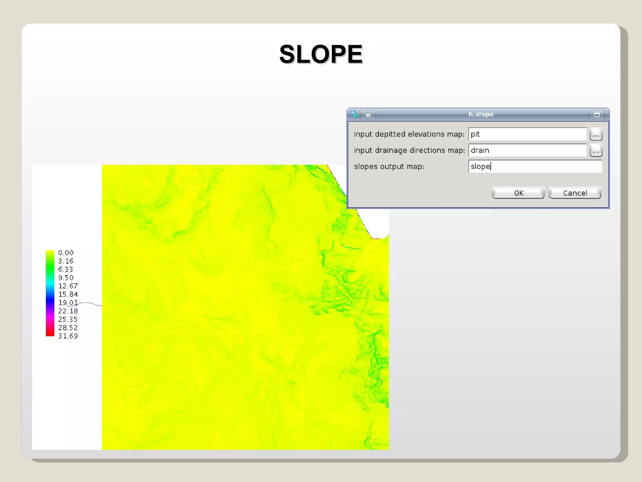
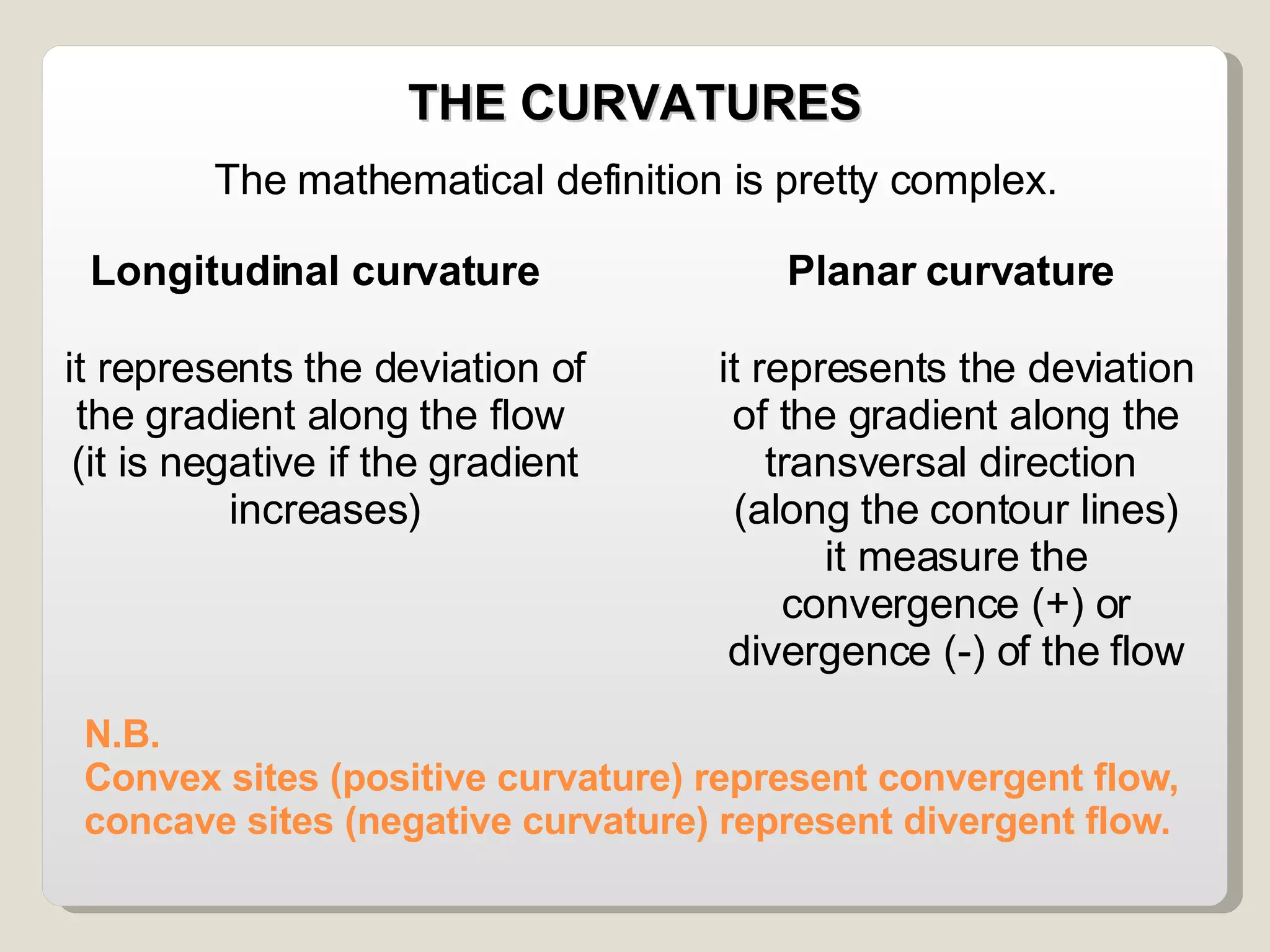
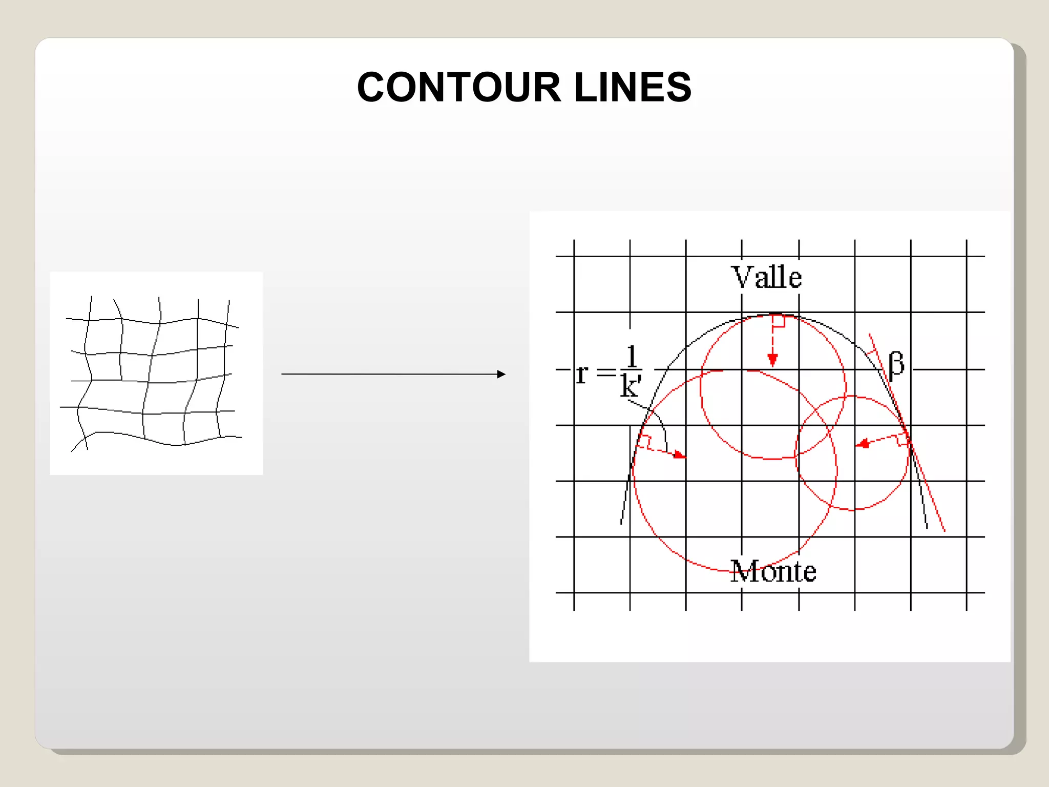
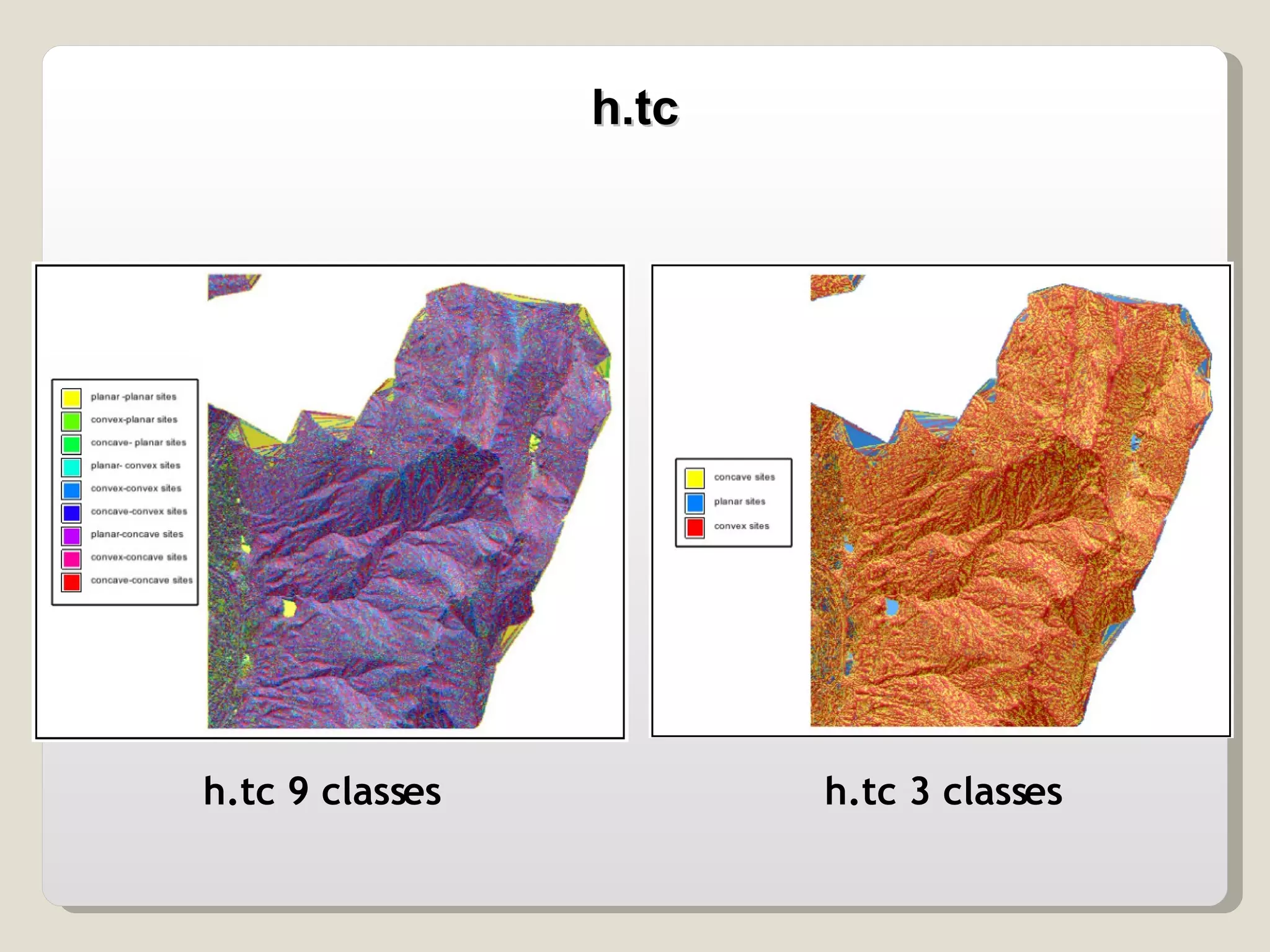
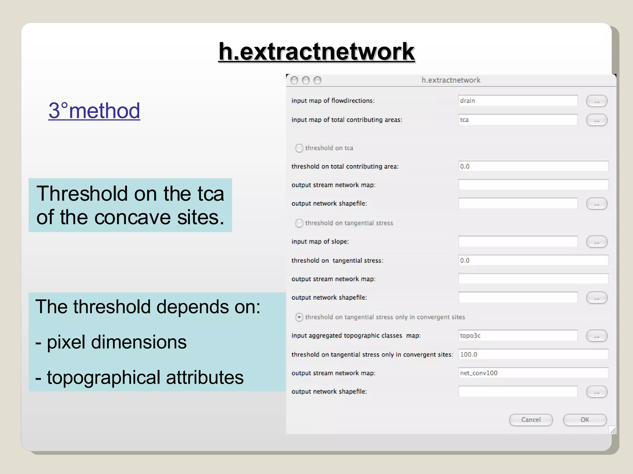
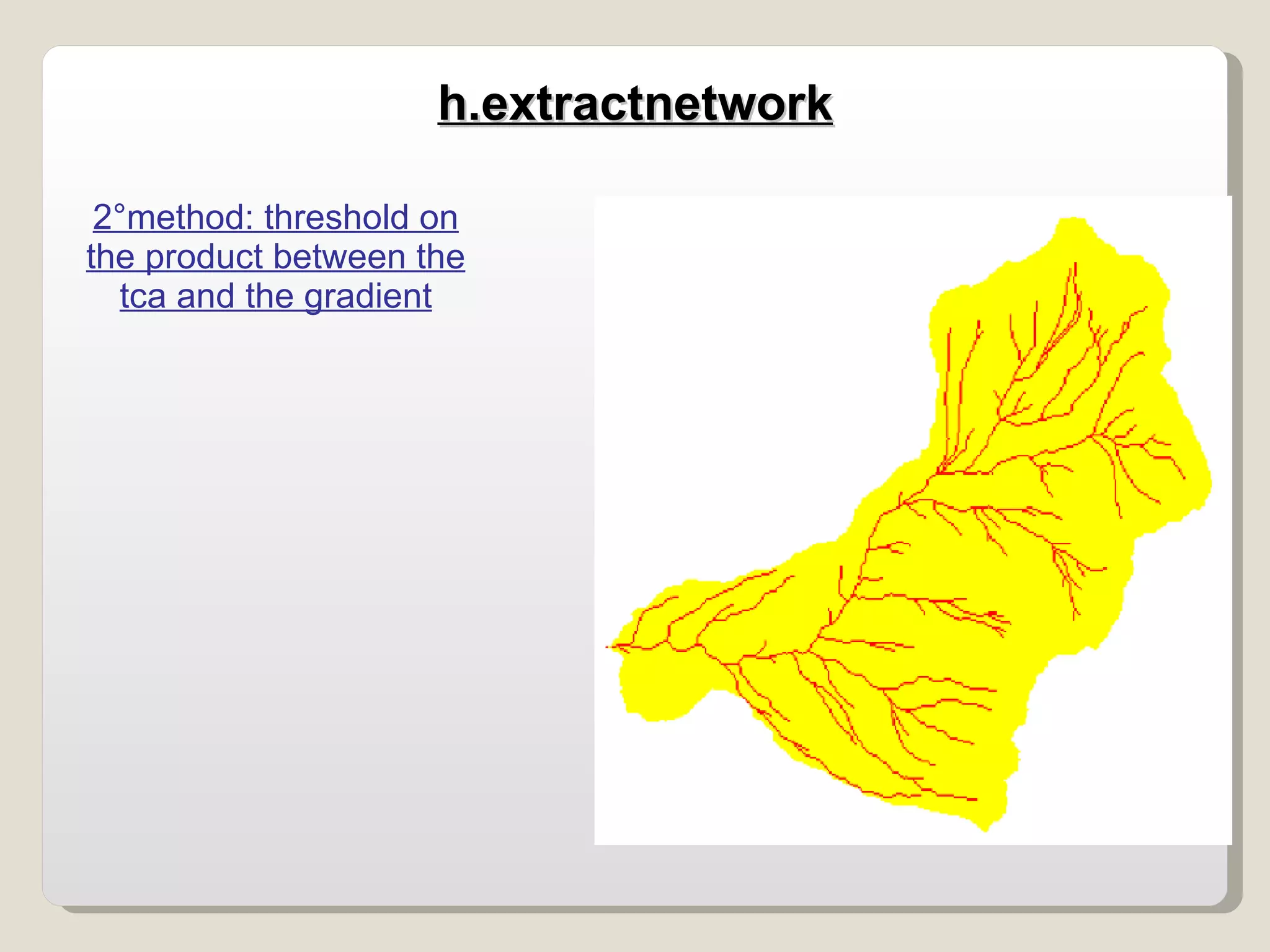
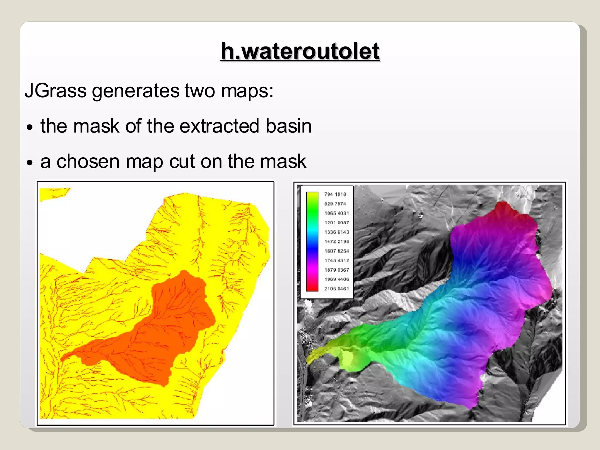
PROVINCIA AUTONOMA DI TRENTO Servizo Bacini Montani JGRASS: ANALISI GEOMORFOLOGICHE Trento, 17 Ottobre 2008

It is developed with the purpose of giving some quantitative and qualitative instruments for knowing the morphology of catchments. Main applications are made in alpine catchments of various dimensions (from some km 2 to hundreds km 2 )‏ Applications are made with different type of DEM (IGM 20 metri, PAT 10 m, LaserAltimetric 2 m)‏ HORTONMACHINE: THE PURPOSE

Starting hypothesis is: HORTONMACHINE: OUR WORK Taking into account of this hypothesis the purpose of the work is to analyse the erosion processes, incision processes of the network and the possibility of landslides. This is done considering that the main geomorphological processes in a catchment are: Diffusive erosion on the hillslopes Network's incision processes Landslides Sediment transport in the channels MORPHOMETRY EROSION PROCESSES

HORTONMACHINE: THE HISTORY At the beginning it was a package of stand alone routines operating system independently, written in C using the FluidTurtle libraries and their input/output defined formats. The visualization of the calculated matrices was made with other graphical programs or with Mathematica; The second step was to integrate this routines in the GIS GRASS to have a direct graphical interface in TkTcl; Nowadays with the JGrass development this routines are being rewritten in Java and completely integrated in the new GIS system with a new development model (OpenMI) and new graphical interface.

HORTONMACHINE: The commands are divided in 7 categories: DEM manipulation

HORTONMACHINE: The commands are divided in 7 categories: DEM manipulation Basic topographic attributes

HORTONMACHINE: The commands are divided in 7 categories: DEM manipulation Basic topographic attributes Network related measures

HORTONMACHINE: The commands are divided in 7 categories: DEM manipulation Basic topographic attributes Network related measures Hillslope analyses

HORTONMACHINE: The commands are divided in 7 categories: DEM manipulation Basic topographic attributes Network related measures Hillslope analyses Basin attributes

HORTONMACHINE: The commands are divided in 7 categories: DEM manipulation Basic topographic attributes Network related measures Hillslope analyses Basin attributes Statistic

HORTONMACHINE: The commands are divided in 7 categories: DEM manipulation Basic topographic attributes Network related measures Hillslope analyses Basin attributes Statistic Hydro-geomorphology

The topography is represented by a bivariate continuous function z = f(x,y) and with continuous derivative up to the second order almost everywhere. MORPHOLOGY

The representation on a regular rectangular grid of the data constitutes the most common and most efficient form in which the terrain digital data can be found. HYPOTHESIS ON DEM: data are significant regular squared grid 8 direction topology DIGITAL ELEVATION MODELS (D.T.M.)‏ The data in this raster form usually is made by reporting the vertical coordinate, z, for a subsequent series of points, along an assigned regular spacing profile.

definition the working region pit detection definition of the drainage directions definition of the main network extraction of the interesting catchment D8 (maximum slope)‏ D8 with correction (correction on the direction of the gradient)‏ PRELIMINARY OPERATIONS import in JGrass the starting DEM which we want to analyse individuation of the existing sub basins

DERIVED ATTRIBUTES: Local slope (h.slope)‏ Local curvature (h.tapes o h.nabla)‏ Total contributing area (h.tca, h.multitca)‏ Catchment divide distance (h.hacklength)‏ Distance to outlet (h.distance2outlet)‏ ……… ..

FIRST STEP: DEPITTING THE DEM The first operation to do is to fill the depression points present within a DEM so that the drainage directions can be defined in each point. Observations on this topic demonstrate that this calculation addresses lesser than the 1% of the data and that usually this depressions are given by wrong calculation in the DEM creation phase and that in fact they are not real depressions. The command used to fill the depressions is: h.pitfiller based on the Tarboton algorithm.

h.pitfiller Fills the depressions following the Tarboton algorithm.

FLOW DIRECTIONS They define how water moves on the surface in relation to the topology of the study region. Flow directions allow you to calculate the drainage directions. Hypothesis: each DEM cell drains only in one of its 8 neighbours, either adjacent or diagonal in the direction of the steepest downward slope. only 8 possible direction in which direct the flux this is a limit of modelling the natural flow

h.flowdirections It calculates the flow direction in the direction of the steepest downward slope choosing for each DEM cell to one of its 8 neighbours. The flow directions convention numbers are from 1 to 8 where 1 is the east direction.

FLOW DIRECTIONS In the map each colour represents one of the 8 drainage directions. The map contains the convention number of this directions.

A CORRECTION TO THE PURE D8 METHOD Using the “pure” D8 method for the drainage direction estimation cause an effect of deviation from the real direction identified by the gradients. This algorithm calculates the drainage direction minimizing the deviation of the flow from the real flux direction. The deviation is calculated beginning from the pixel at highest elevation and going downstream. The deviation is calculated with a triangular construction and can be expressed as angular deviation (method D8-LAD) or as transversal distance (method D8-LTD)‏ The lambda parameter is used to assign a weight to the correction made to the drainage directions. This method has been developed by S. Orlandini

h.draindir LAD method: angular deviation LTD method: transversal deviation The deviation is cumulated from higher pixels down-hill and the D8 drainage direction is redirected to the real direction when the value is larger than an assigned threshold. If λ = 0 the deviation counter has no memory and the pixels up-hill do not affect the choice.

THE NEW DRAINAGE DIRECTIONS AND THE NEW TCA STANDARD METHOD

h.draindir Map obtained categorizing the resulting map of the command Map obtained personalizing the colours of the original map

h.draindir NETWORK FIXED METHOD: in flat areas or where there are manmade constructions, it can happen that the extracted channel network does not coincide with the real channel network.

TOTAL CONTRIBUTING AREA It represents the area that contributes to a particular point of the catchment basin. It is an extremely important quantity in the geomorphologic and hydrologic study of a river basin: it is strictly related to the discharge flowing through the different points of the system in uniform precipitation conditions. On this quantity most of the diffusive methods used to extract the stream network from the digital models are based.

TCA Where W j is: 1 for pixels that drain into the i-est pixel; 0 in any other case for single flow directions.

TCA 1 2 3 4 5 6 7 8 9 Where W j is: 1 for pixels that drain into the i-est pixel; 0 in any other case for single flow directions. source

TCA RESULTS COMPARISON In the figures are compared the total contributing areas calculated with the pure D8 method and with the corrected method (LAD-D8). In the second case the typical maximum steepest parallelisms are not present with a representation of the flow very near to reality. Log(TCA)‏ Log (LAD-TCA)‏

FLOW DIRECTIONS Many applications to be correctly executed need a matrix of the flow directions that have a new class value. This new class (conventionally indicated in JGrass with 10) identifies the basin outlets, those are the pixels draining outside the analysed region. In other words this command marks the outlets: The command is:

GRADIENTS The gradients are relevant because the main driving force of the flux is the gravity and the gradient identifies the flow directions of the water and contributes also to determinate its velocity. Let's observe that the gradient, contrarily to the slope, does not use the drainage directions. It calculates only the module of the gradient which in reality is a vectorial quantity oriented in the direction starting from the minimal up to the maximal potential.

We can see the deep network incision and the flat area near the basin outlet. The particular wrong calculation in the upper part of the basin is due to the union of the originally squared DEM. GRADIENTS

The gradient calculated whit this command is given as the tangent of the correspondent angle. Using the MAPCALCULATOR it is possible to obtain the map of the gradients in degrees: atan(gradient)*180/3.14 h.gradient

The gradient calculated whit this command is given as the tangent of the correspondent angle. Using the MAPCALCULATOR it is possible to obtain the map of the gradients in degrees: atan(gradient)*180/3.14 new_map = if (condition, then, else)‏ h.gradient

It estimates the slope in every site by employing the drainage directions. Differently from the gradients, slope calculates the drop between each pixel and the adjacent points placed underneath and it divides the result by the pixel length or by the length of the pixel diagonal, according to the cases. The greatest value is the one chosen as slope. SLOPE

N.B. Convex sites (positive curvature) represent convergent flow, concave sites (negative curvature) represent divergent flow. THE CURVATURES The mathematical definition is pretty complex. Longitudinal curvature Planar curvature it represents the deviation of the gradient along the flow (it is negative if the gradient increases)‏ it represents the deviation of the gradient along the transversal direction (along the contour lines)‏ it measure the convergence (+) or divergence (-) of the flow

h.curvatures Longitudinal Curvature Planare Curvature The planar curvatures separate the concave parts from the convex ones The longitudinal curvatures highlight valleys

TOPOGRAPHIC CLASSIFICATION It subdivides the sites of a basin in the 9 topographic classes identified by the longitudinal and transversal curvatures. The aggregation of the classes in the three fundamentals index: CONCAVE SITES CONVEX SITES PLANAR SITES

h.tc The program asks as input the threshold values of the longitudinal and normal curvatures which define their planarity. THE VALUE IS STRICTLY RELATED TO THE TOPOLOGY

h.tc h.tc 9 classes h.tc 3 classes

CHANNEL NETWORK EXTRACTION 3 METHODS ARE IMPLEMENTED threshold value on the contributing areas (only the pixels with contributing area greater than the threshold are the channel heads)‏ threshold value on the stress tangential at the bottom: threshold value on the ratio between the total contributing areas and the gradient threshold value on the tangential stress only in convergent sites HOW IT WORKS: As soon as the first pixel of the channel network (the pixel in which the value of the parameter is larger than the threshold) is found, all the other pixel downstream are network.

h.extractnetwork Threshold on the tca The threshold depends on: - dimensions of the pixels - topographical attributes 1°method

The threshold depends on: - pixels dimensions - topographical attributes 2°method h.extractnetwork The threshold is on the parameter: which is proportional to the stress tangential to the bottom.

Threshold on the tca of the concave sites. The threshold depends on: - pixel dimensions - topographical attributes 3°method h.extractnetwork

In the resulting raster map the network pixels have the 2 value and outside the network there are null values. 1°method: threshold on the tca h.extractnetwork

2°method: threshold on the product between the tca and the gradient h.extractnetwork

3°method: threshold on the tca in the concave pixels In this case there are various groups of stream networks, everyone of them corresponds to a catchment. h.extractnetwork

ESTRACTION OF THE WORKING BASIN first give the basin outlet: insert known coordinates of a point use the Query raster tool to select a point directly on the network map and verify that the point is on the net (has a value of 2)‏. The coordinates of this point will be added to the clipboard. use the coordinates of the selected outlet in the h.wateroutlet command

JGrass generates two maps: the mask of the extracted basin a chosen map cut on the mask h.wateroutolet

h.pitfiller h.flowdirection h.draindir h.wateroutlet h.gradient h.curvatures h.tc h.extractnetwork BASIN MORPHOLOGICAL ANALYSIS First of all we have to execute the previous commands only for the extracted basin. Another choice would be to cut the maps on the extracted mask with the command mapcalculator .

drainage directions total contributing area extracted network gradient curvatures topographic classes BASIN MORPHOLOGICA ANALYSIS The best thing to do is to cut the original maps on the extracted basin mask. The maps to cut are the following:

h.ab It calculates the draining area per length unit (A/b), where A is the total upstream area and b is the length of the contour line which is assumed as drained by the A area. The contour length is here be estimated by a a novel method based on curvatures.

h.ab The stream network pixels are the concave sites. concave sites convergent sites convex sites divergent sites The contour line is locally approximated by an arc having the radius inversely proportional to the local planar curvature b ~ t'

The higher values of A/b are registered near on the channel network. In fact those are the points in which the contributing area is the highest and the value of b is the lowest. THE RESULT OF A/B

THE RESULT OF A/B CHANGING THE COLORMAP

ESPOSIZIONE Calculates for every point the aspect, defined as the inclination angle of the gradient. The considered reference system put the angle to zero when the gradient is orientated towards east and grows counter-clock-wise. The value angle is calculated in radiants. Mathematical formula:

It is defined as the area upstream that drains into the current point. A large part of DEM related literature analyses this parameter and its determination. Usually it is calculated taking into consideration the steepest slope, but a single flowdirection for every point is not enough to have an accurate description of the runoff. A solution to this problem is the use of an algorithm that introduces multiple draining directions on the hillslope and single ones for concave sites. THE TOTAL CONTRIBUTING AREA

where: W j is 1 for sites that drain into the i-est site 0 otherwise in the case of multiple drainage directions instead we have: 0 ≤ W j ≤1 -> in which case: Where k represents the number of sites into which the j-est point drains. h.tca h.multitca THE TOTAL CONTRIBUTING AREA

N.B. Concave sites (positive curvature) represent converging flux, convex sites (negative curvature) represent diverging flux. Laplacian is a strict relative of the curvatures and gives a way to distinguish in a first iteration convex and concave sites of the catchment. Mathematical definition: FIRST APPROACH TO CURVATURES: LAPLACIAN

convex element flat element concave element Positive curvature Negative curvature Null curvature DEFINITIONS FOR CURVATURES

It estimates the longitudinal (or profile), normal and planar curvatures for each site through a finite difference schema. longitudinal curvature represent the deviation of the gradient along the the flow (it is negative if the gradient increase), the normal and planar curvatures are locally proportional and measure the convergence/divergence of the flow (the curvature is positive for convergent flow). h.curvatures

It subdivides the sites of a basin in 11 topographic classes. nine classes based obtained with TC h.gc

It subdivides the sites of a basin in 11 topographic classes. nine classes based obtained with TC the points belonging to the channel networks constitute a tenth class (derived from the use of ExtractNetwork) the points with high slope (higher than a critical angle) the eleventh class. h.gc

THE DISTANCES BY HACK It is given, assigned a point in the catchment, by the projection of the distance from the catchment divide along the network (until it exists), and then, proceeding upstream along the maximal slope lines. For each network confluence, the direction of the tributary with maximal contributing area is chosen. If the tributaries have the same area, one of the two directions is chosen at random.

MAGNITUDO: h.magnitudo The magnitude is defined as the number of sources upstream to every point of the catchment. If the river net is a trifurcated tree (a node in which three channels enter and one exits), then between number of springs and channels there exists a bijective correspondence hc = 2ns − 1 hc is the number of channels ns the number of sources The mangitudo is also an indicator of the contributing area.

NETNUMBERING It assign numbers to the network’s links. It can be used by hillslope2channelattribute to label the hillslope flowing into the link with the same number.

SUBBASIN EXTRACTION: h.netnumbering The subbasins depend on the complexity of the network: a complex network has a large number of subbasins a simple network has a small number of subbasins

THE DISTANCE FROM THE NETWORK Evaluates the distance of every pixel in the catchment to the network. It can work in 2 different ways: calculates the distance in pixels calculates the distance in meters

h.hillslope2channeldistance Distance map for a simple channel network Distance map for a rather complex channel network

HYDRO-GEOMORPHOLOGY: h.shalstab It is a version of the shalstab model, which uses a simplified hydrological model and the model of infinite slope to evaluate a stability coefficient. The variables considered are: the area contributing in one point b the length of the boundary in the point considered S the soil density w the water density the angular slope the friction angle T the soil transmissivity q the effective rain

HYDRO-GEOMORPHOLOGY: h.shalstab It is a version of the shalstab model, which uses a simplified hydrological model and the model of infinite slope to evaluate a stability coefficient. The variables considered are: the area contributing in one point b the length of the boundary in the point considered S the soil density w the water density the angular slope the friction angle T the soil transmissivity q the effective rain.

Corso Pat Jgrasshorton 2008 10 17

More Related Content

What's hot

Viewers also liked

Similar to Corso Pat Jgrasshorton 2008 10 17

More from silli

Recently uploaded

Corso Pat Jgrasshorton 2008 10 17