Download as PDF, PPTX
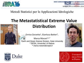
![Classical Extreme Value Theory (EVT)
[Fischer-Tippett-Gnedenko, 1928-1943]
Block Maxima:
Three-Type Theorem:
- As n ∞
-After renormalization, 3 possible
asymptotic distributions,
summarized by GEV (e.g. Von Mises, 1936):
= Maxima n-event blocks
h[mm]
𝑥 𝑛
1937 19381936 1939 194019411942
𝑥 𝑛 = max
𝑛
(𝑥𝑖)
for i.i.d 𝑥𝑖 ∶ 𝐻 𝑛 𝑥 = 𝐹 𝑥 𝑛
𝐻 𝑥 = exp − 1 +
𝜉
𝜓
𝑥 − 𝜇
+
−
1
𝜉](https://image.slidesharecdn.com/zorzettobottermaraniidra2016mev-160921115004/85/Metastatistical-Extreme-Value-distributions-2-320.jpg)
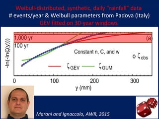
![A choice for F(x) - the pdf of daily «ordinary» rainfall
𝑅 𝑎𝑐𝑐 = ത𝑘ത𝑞𝑚
𝐹 𝑥 = 1 − 𝑒
𝑥
𝐶
𝑤 Weibull Parent
distribution
ത𝑘=precipitation efficiency
ത𝑞=specific humidity
m=advection mass
[Wilson e Tuomi, 2005]
-Simple two-layers atmospheric model
-Temporal average](https://image.slidesharecdn.com/zorzettobottermaraniidra2016mev-160921115004/85/Metastatistical-Extreme-Value-distributions-8-320.jpg)


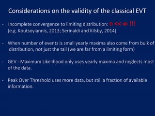
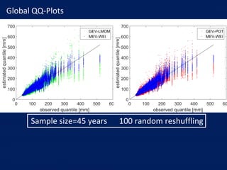
![Method of analysis
• To eliminate correlation and non-stationarity
• Preserving the true (unknown) distribution of the
parameters and numbers of wet days.
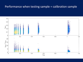
• Fit on a sample of size s
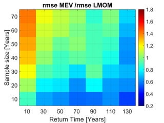
• Test on remaining data. Non dimensional Root
Mean Square Error:
Which is studied as a function of sample size s.
Bootstrap - Reshuffling of daily data preserving
(1) yearly number of events, and
(2) observed values (i.e. Pdf’s)
ORIGINAL TIME SERIES
𝜖 =
1
𝑁
(
ො𝑥 − 𝑥 𝑜𝑏𝑠
𝑥 𝑜𝑏𝑠
)2
RANDOMLY RESHUFFLED TIME SERIES
T Years
h [mm]
h [mm]
t [days]
t [days]](https://image.slidesharecdn.com/zorzettobottermaraniidra2016mev-160921115004/85/Metastatistical-Extreme-Value-distributions-12-320.jpg)


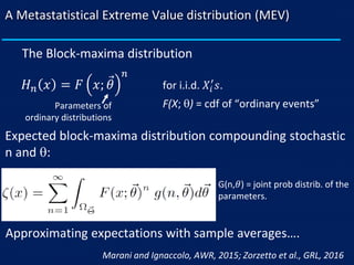
![N
1982 1986198519841983
t
h [mm]
𝑛1 = 97 𝑛2 = 105 𝑛3 = 89 𝑛4 = 94 𝑛5 = 114
𝐶1, 𝑤1 𝐶2, 𝑤2 𝐶3, 𝑤3 𝐶4, 𝑤4 𝐶5, 𝑤5
2. Fit Weibull to the singl𝑒 𝑦𝑒𝑎𝑟𝑠 𝐶𝑖, 𝑤𝑖
1. Sampling n from the distribution p(n|C,w)
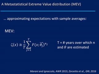
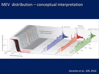
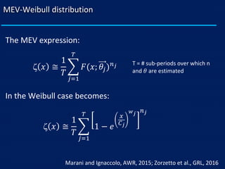
The MEV distribution
𝐹 𝑥 = 1 − 𝑒
𝑥
𝐶
𝑤
• Assuming Weibull as a pdf for daily rainfall
• Fit performed using Probability Weighted Moments (Greenwood et al, 1979)
Number of
events/ year](https://image.slidesharecdn.com/zorzettobottermaraniidra2016mev-160921115004/85/Metastatistical-Extreme-Value-distributions-26-320.jpg)


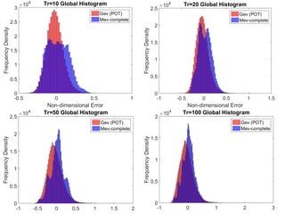
![Peak Over Threshold Method (POT)
[Balkema, De Haan & Pickand, 1975; Davison and Smith, 1990]
• Exceedances arrivals Poisson
• Distribution of excesses Generalized Pareto
Advantages:
1. Better description of the ‘tail’
2. Consistent with GEV
𝑃 𝑌 𝑚𝑎𝑥 < x =
𝑛=1
∞
𝑝 𝑛 ⋅ 𝐹 𝑥 𝑛
=
𝑛=1
∞
𝜆 𝑛
𝑒−𝑛
𝑛!
∙ 1 − 1 +
𝜉
𝜓
∙ 𝑥 − 𝑞
−1/𝜉
𝑛
For a fixed threshold q → Exceedances 𝑌𝑖 = 𝐻𝑖 − 𝑞 𝑖. 𝑖. 𝑑. 𝑟. 𝑣.
𝑦𝑖 = ℎ𝑖 − 𝑞](https://image.slidesharecdn.com/zorzettobottermaraniidra2016mev-160921115004/85/Metastatistical-Extreme-Value-distributions-32-320.jpg)


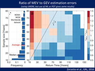
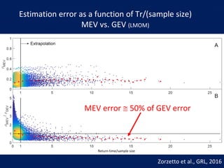
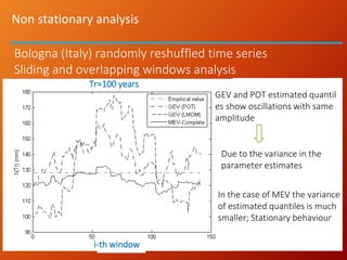
- The document presents the Metastatistical Extreme Value (MEV) distribution as an improvement over classical extreme value theory. - MEV accounts for the stochasticity in both the number of rainfall events per year and the parameters of the underlying rainfall distribution. This better represents scenarios with limited data where the asymptotic assumptions of classical methods break down. - The author applies MEV using a Weibull distribution for daily rainfall and finds it outperforms generalized extreme value and peak over threshold methods by reducing estimation errors of rainfall quantiles by around 50% on average across diverse datasets.


