2. X. Li, M. Yin
posed in 2009. The cuckoo search algorithm is a population-
based heuristic evolutionary algorithm inspired by the inter-
esting breeding behavior such as brood parasitism of certain
species of cuckoos. In CS, each cuckoo lies on egg at a time
and dumps its egg in a randomly chosen nest. The best nests
with high quality of eggs will carry over to the next genera-
tion. The number of available host nests is fixed, and the egg
laid by a cuckoo is discovered by the host bird with a prob-
ability. In this case, the host bird can either abandon the egg
away or throw the nest, and build a completely new nest. To
accelerate the convergence speed and avoid the local optima,
several variations of CS have been proposed to enhance the
performance of the standard CS recently. Moreover, CS has
been proved to be really efficient when solving real-world
problems. Civicioglu (2013a,b) compares the performance
of CS with that of particle swarm optimization, differential
evolution, and artificial bee colony on many global optimiza-
tion problems. The performances of the CS and PSO algo-
rithms are statistically closer to the performance of the DE
algorithm than the ABC algorithm. The CS and DE algo-
rithms supply more robust and precise results than the PSO
and ABC algorithms. Walton et al. (2011) proposes modi-
fied cuckoo search which can be regarded as a modification
of the recently developed cuckoo search is presented. The
modification involves the addition of information between
the top eggs, or the best solutions. Gandomi et al. (2013)
proposes the CS for solving structural optimization prob-
lems which is subsequently applied to 13 design problems
reported in the specialized literature. The performance of
the CS algorithm is further compared with various algo-
rithms representative of the state of the art in the area. The
optimal solutions obtained by CS are better than the best
solutions obtained by the existing methods. Layeb (2011)
proposes a new inspired algorithm called quantum inspired
cuckoo search algorithm, which a new framework is relying
on quantum computing principles and cuckoo search algo-
rithm. The contribution consists in defining an appropriate
representation scheme in the cuckoo search algorithm that
allows applying successfully on combinatorial optimization
problems. Tuba et al. (2011) implements a modified version
of this algorithm where the stepsize is determined from the
sorted rather than only permuted the fitness matrix. The mod-
ified algorithm is tested on eight standard benchmark func-
tions. Comparison of the pure cuckoo search algorithm and
this modified one is presented and it shows improved results
by the modification. Goghrehabadi et al. (2011) proposes a
hybrid power series and cuckoo search via lévy flights opti-
mization algorithm (PS-CS) that is applied to solve a system
of nonlinear differential equations arising from the distrib-
uted parameter model of a micro fixed–fixed switch subject
to electrostatic force and fringing filed effect. The obtained
results are compared with numerical results and found in
good agreement. Furthermore, the present method can be
easily extended to solve a wide range of boundary value
problems. Yildiz (2013a,b) proposes CS to the optimization
of machining parameters. The results demonstrate that the
CS is a very effective and robust approach for the optimiza-
tion of machining optimization problems. Durgun and Yildiz
(2012) proposed to use the cuckoo search algorithm (CS)
algorithm for solving structural design optimization prob-
lems. The CS algorithm is applied to the structural design
optimization of a vehicle component to illustrate how the
present approach can be applied for solving structural design
problems. Agrawal et al. (2013) use the cuckoo search algo-
rithm to find the optimal thresholds for multi-level threshold
in an image are obtained by maximizing the Tsallis entropy.
The results are then compared with that of other compared
algorithms. Ouaarab et al. (2014) present an improved and
discrete version of the cuckoo search (CS) algorithm to solve
the famous traveling salesman problem (TSP), an NP-hard
combinatorial optimization problem. The proposed discrete
cuckoo search (DCS) is tested against a set of benchmarks
of symmetric TSP from the well-known TSPLIB library.
Burnwal and Deb (2013) propose a new algorithm to solve
scheduling optimization of a flexible manufacturing system
by minimizing the penalty cost due to delay in manufactur-
ing and maximizing the machine utilization time. Li et al.
(2014) use a new search strategy based on orthogonal learn-
ing strategy to enhance the exploitation ability of the basic
cuckoo search algorithm. Experiment results show that the
proposed algorithm is very effective. Dey et al. (2013) pro-
pose a new approach to design a robust biomedical content
authentication system by embedding logo of the hospital
within the electrocardiogram signal by means of both dis-
crete wavelet transformation and cuckoo search algorithm.
An adaptive meta-heuristic cuckoo search algorithm is used
to find the optimal scaling factor settings for logo embedding.
Ehsan and Saeed (2013) use an improved cuckoo search algo-
rithm, enhancing the accuracy and convergence rate of the
standard cuckoo search algorithm. Then, the performance
of the proposed algorithm is tested on some complex engi-
neering optimization problems including four well-known
reliability optimization problems and a large-scale reliabil-
ity optimization problem, which is a 15-unit system reliabil-
ity optimization problem. These methods seem to be dif-
ficult to simultaneously achieve the balance between the
exploration and exploitation of the CS. Therefore, a large
number of future researches are necessary to develop new
effective cuckoo search algorithms for optimization prob-
lems.
To achieve both of the goals, the proposed algorithm
inspired by the particle swarm optimization is used for the
best individuals among the entire population. While the PSO
directly uses the global best solution of the population to
determine new positions for the particles at the each iter-
ation, agents of the CS do not directly use this informa-
123
3. A particle swarm inspired cuckoo search algorithm
tion but the global best solution in the CS is stored at the
each iteration. Therefore, in the first component, the neigh-
borhood information is added into the new population to
enhance the diversity of the algorithm. In the second com-
ponent, two new search strategies are used to balance the
exploitation and exploration of the algorithm through a ran-
domly probability rule. In other aspect, our algorithm has
a very simple structure and thus is easy to implement. To
verify the performance of PSCS algorithm, 30 benchmark
functions chosen from literature are employed. Compared
with other evolution algorithms from literature, experimental
results indicate that the proposed algorithm performs better
than, or at least comparable to state-of-the-art approaches
from literature when considering the quality of the solu-
tion obtained. In the last, experiments have been conducted
on two real world problems. Simulation results and com-
parisons demonstrate the proposed algorithm is very effec-
tive.
The rest of this paper is organized as follows: In Sect. 2
we will review the basic CS and the basic PSO. The parti-
cle swarm inspired cuckoo search algorithm is presented in
Sect. 3 respectively. Benchmark problems and correspond-
ing experimental results are given in Sect. 4. Two real world
problems are given in Sect. 5. In the last section we conclude
this paper and point out some future research directions.
2 Preliminaries
2.1 The standard cuckoo search algorithm
Cuckoo search algorithm was first proposed by Yang and
Deb (2009). The algorithm was one of the most recent swarm
intelligent-based algorithms that were inspired by the oblig-
ate brood parasitism of some cuckoo species by laying their
eggs in the nests of other host birds. In the standard cuckoo
search algorithm, the algorithm combines three principle
rules. First, each cuckoo will be dumped in a randomly cho-
sen nest. The second rule is that the best nests will be kept
to the next generation. The third rule is that the host bird
will find the egg laid by a cuckoo with a probability. When
it happens, the laid egg will be thrown away or the host bird
will abandon the nest to build a new nest. Based on these
rules, the standard cuckoo search algorithm is described as
follows:
Inthebeginningofthecuckoosearchalgorithm,eachsolu-
tion is generated randomly within the range of the boundary
of the parameters. When generating ith solution in t + 1
generation, denoted by xt+1
i , a lévy flight is performed as
follows:
xt+1
i = xt
i + α ⊕ Le vy(λ) (1)
where α > 0 is real number denoting the stepsize, which is
related to the sizes of the problem of interest, and the product
⊕ denotes entry-wise multiplications. A lévy flight is a ran-
dom walk where the step-lengths are distributed according to
a heavy-tailed probability distribution in the following form:
le vy ∼ u = t−λ
, (1 < λ < 3), (2)
which has an infinite variance with an infinite mean. Accord-
ingly, the consecutive jumps of a cuckoo from a random walk
process obeying a power law step length distribution with a
heavy tail. In this way, the process of generating new solu-
tions can be viewed as a stochastic equation for random walk
123
4. X. Li, M. Yin
which also forms a Markov chain whose next location only
depends on the current location and the transition probability.
The evolution phase of the xt
i begins by the donor vector
υ, where υ = xt
i . After this step, the required stepsize value
has been computed using the Eq. (3)
Stepsizej = 0.01 ·
u j
vj
1/λ
· (υ − Xbest) (3)
where u = t−λ × randn[D] and v = randn[D]. The
randn[D] function generates a Gaussian distribution. Then
the donor vector υ is random using the Eq. (4)
υ = υ + Stepsizej ∗ randn[D] (4)
After producing the new solution υi , it will be evaluated and
compared to the xi , If the objective fitness of υi is smaller
than the objective fitness of xi , υi is accepted as a new basic
solution. Otherwise xi would be obtained.
The other part of cuckoo search algorithm is to place some
nests by constructing a new solution. This crossover operator
is shown as follows:
υi =
Xi + rand · (Xr1 − Xr2) randi < pa
Xi otherwise
(5)
After producing the new solution υi , it will be evaluated and
compared to the xi . If the objective fitness of υi is smaller
than the objective fitness of xi , υi is accepted as a new basic
solution. Otherwise xi would be obtained.
Note that in the real world, a cuckoo’s egg is more difficult
to be found when it is more similar to a host’s eggs. So, the
fitness is related to the difference and that is the main reason
to use a random walk in a biased way with some random
stepsizes.
2.2 The particle swarm optimization algorithm (PSO)
PSO is fundamentally a stochastic, population-based search
algorithm which mimics organisms that interact as a swarm
such a school of fish or a swarm of bees looking for the foods.
The algorithm was first proposed by Kennedy and Eberhart
(1995)basedonthecooperationandcompetitionamongindi-
viduals to complete the search of the optimal solution in an
n-dimensional space. The standard PSO can be specifically
described as follows: during the swarm evolution, each parti-
cle has a velocity vector Vi = (vi1, vi2, . . . , vi D) and a posi-
tionvector Xi = (xi1, xi2, . . . , xi D) toguideitself toapoten-
tial optimal solution, wherei is a positive integer indexing the
particle in the swarm. The personal best position of particle
i is denoted as pbesti = (pbesti1, pbesti2, . . . , pbesti D)
and the global best position of the particle is gbest =
(gbest1, gbest2, . . . , gbestD). The velocity Vi and the posi-
tion xi are randomly initialized in the search space and they
are updated with the following formulas at the (t + 1) gen-
erations:
Vi, j (t + 1) = ωVi, j (t) + c1r1, j pbesti, j (t) − Xi, j (t)
+ c2r2, j gbestj (t) − Xi, j (t)
Xi, j (t + 1) = Xi, j (t) + Vi, j (t + 1) (6)
where i ∈ [1, 2, . . . , N P] means the ith particle in the pop-
ulation and j ∈ [1, 2, . . . , D] is the jth dimension of this
particle; NP is the population size and D is the dimension of
the searching space. c1 and c2 are acceleration constants. The
r1, j and r2, j are two random number uniformly distributed
in [0, 1]. ω is the inertia weight that is used to balance global
and local search ability.
3 Our approach: particle swarm inspired cuckoo search
algorithm (PSCS)
In this section, we will introduce our algorithm PSCS in
detail.
3.1 The new search strategy
In the standard PSO algorithm, each particle keeps the best
position pbest found by itself. Besides, we know the global
position gbest search by the group particles, and change its
velocity according to the two best positions. The high con-
vergence speed is an important feature of the original PSO
algorithm because of the usage of the global elite “gbest”
imposes a strong influence on the whole swarm. The global
best solution is used to guide the flight of the particles, as it
can be called “social learning”. In the social learning part,
the individuals’ behaviors indicate the information share and
cooperation among the swarm. The other learning part is the
cognitive learning models which make the tendency of parti-
cles to return to previously found best positions. This part can
avoid the algorithm trapping into the local optimal. Inspired
by the social learning and cognitive learning, the two learn-
ing parts are used in standard CS to find the neighborhood of
the nest. The main model of the new search strategy can be
described as follows:
υi, j (t + 1) = Xi, j (t) + ϑi, j pbesti, j (t) − Xi, j (t)
+ ϕi, j gbestj (t) − Xi, j (t) (7)
where ϑ and ϕ are the parameter of the new search method.
In other aspect, as the global best found early in the search-
ing process may be a poor local optimum; it may attract all
food sources to a bad searching area. In this case, on com-
plex multi-modal problems, the convergence speed of the
algorithm is often very high at the beginning, but only lasts
for a few generations. After that, the search will inevitably
be trapped. Therefore, on such kind of problems, it would
mislead the search towards local optima, which inhibits the
advantages of the new strategies on multi-modal problems. In
123
5. A particle swarm inspired cuckoo search algorithm
this paper, taking into consideration these facts and to over-
come the limitations of fast but less reliable convergence
performance of the above search strategy, we propose a new
search strategy by utilizing the best vector of a group of q%
of the randomly selected population members for each target
vector that can be described as follows:
υi, j (t + 1) = Xi, j (t) + ϑi, j pbesti, j (t) − Xi, j (t)
+ ϕi, j q_gbestj (t) − Xi, j (t) (8)
where q_gbest is the best of the q% vectors randomly cho-
sen from the current population, and none of them is equal
to q_gbest. Under this method, the target solutions are not
always attracted toward the same best position found so far in
the current population, and this feature is helpful in avoiding
premature convergence at local optima. It is seen that keeping
the value of the q% is equal to the top 5 % of the population
size.
In the standard CS algorithm, two main components com-
bine the algorithm. The first component of algorithm gets
new cuckoos by random walk with Lévy flight around the so
far best nest. The required stepsize value has been computed
as follows:
Stepsizej = 0.01 ·
u j
vj
1/λ
· (υ − Xbest) (9)
where u = σu × randn[D] and v = randn[D]. The
randn[D] function generate an rand number between [0,1].
Then the donor vector υ can be generated as follows:
υ = υ + Stepsizej ∗ randn[D] (10)
Inspired by the new search strategy, we can modify the first
part as follows:
υ = υ + 0.01 ·
u j
vj
1/λ
· (υ − q_gbest) ∗ randn[D]
+ ϕ ∗ (Xr1 − q_gbest) (11)
wherer1 ismutuallydifferentrandomintegerindicesselected
from {1, . . . , N P}. ϕ is the parameter of this part. From the
new modified search method, we can find that the first part
shows the distance of the current individual and the global
best individual. The second part shows the distance of the
neighborhood of the current individual and the global best
individual. This new search strategy can enhance the conver-
gence rate and the diversity of the population. It can avoid
the algorithm trapping into the local optimal.
For the second component of cuckoo search algorithm,
the nest can place some nests by construct a new solution.
This crossover operator is shown as follows:
υi =
Xi + rand · (Xr1 − Xr2) randi < pa
Xi otherwise
(12)
Inspired by the new search strategy, in this section, two
improved search strategies are used in the second compo-
nent of the cuckoo search algorithm.
υi, j (t + 1) = Xi, j (t) + ϑi, j Xr1, j (t) − Xi, j (t)
υi, j (t + 1) = Xi, j (t) + ϑi, j Xr1, j (t) − Xi, j (t)
+ ϕi, j q_gbestj (t) − Xi, j (t) (13)
For the first mutation strategy, it is able to maintain popula-
tion diversity and global search capability, but it slows down
the convergence of CS algorithms. For the second mutation
strategy, the best solution in the current population is very
useful information that can explore the region around the best
vector. Besides, it also favors exploitation ability since the
new individual is strongly attracted around the current best
vector and at same time enhances the convergence speed.
However, it is easy to trap into the local minima. Based on
these two new search strategies, the new crossover strategy
is embedded into the cuckoo search algorithm and it is com-
bined with these two new search strategies through a random
probability rule as follows:
If rand > 0.5 Then
υi, j (t + 1) = Xi, j (t) + ϑi, j Xr1, j (t) − Xi, j (t)
Else
υi, j (t + 1) = Xi, j (t) + ϑi, j Xr1, j (t) − Xi, j (t)
+ ϕi, j q_gbestj (t) − Xi, j (t)
End If (14)
It can be found that one of the two strategies is used to
produce the current individual relative to a uniformly distrib-
uted random value within the range (0, 1). Hence, based on
the random probability rule and two new search methods, the
algorithm can balance the exploitation and exploration in the
search space.
3.2 Boundary constraints
The PSCS algorithm assumes that the whole population
should be in an isolated and finite space. During the search-
ing process, if there are some individuals that will move out
of bounds of the space, the original algorithm stops them
on the boundary. In other words, the nest will be assigned
a boundary value. The disadvantage is that if there are too
many individuals on the boundary, and especially when there
exists some local minimum on the boundary, the algorithm
will lose its population diversity to some extent. To tackle
this problem, we proposed the following repair rule:
xi =
⎧
⎨
⎩
2 ∗ li − xi if xi < li
2 ∗ ui − xi if xi > ui
xi otherwise
(15)
123
6. X. Li, M. Yin
3.3 Proposed PSCS algorithm
In this section, we introduce the new proposed particle swarm
inspired cuckoo search algorithm to balance the exploitation
and the exploration. In this modified version, the new search
rules are proposed based on the best individual among the
entire population of a particular generation. In addition, The
PSCS has a very simple structure and thus is easy to imple-
ment and not enhance any complexity. Moreover, this method
can overcome the lack of the exploration of the standard CS
algorithm. The algorithm can be described as follows:
In this section, we will analyze the computational com-
plexity of the new proposed particle swarm inspired cuckoo
search algorithm. As we know, almost all metaheurtics algo-
rithm are simple in terms of complexity, and thus they are
easy to implement. Proposed particle swarm inspired that
cuckoo search algorithm has two stages when going through
the population NP with the dimension D and one outer loop
for iteration Gmax. Therefore, the complexity at the extreme
case is O(2 · N P · D · Gmax). For the new proposed method.
Runtime complexity of finding the top 5 % globally best vec-
tor depends only on comparing the objective function against
123
7. A particle swarm inspired cuckoo search algorithm
the previous function value. Note that the top 5 % values
should be upgraded for each newly generated trial vector. In
the worst cased, this is done 2 · N P · Gmax. Thus, the overall
runtime remains O(max(2·N P ·Gmax, 2·N P · D·Gmax)) =
O(2 · N P · D · Gmax). Therefore, our algorithm does not
impose any serious burden on the runtime complexity of the
existing CS variants. From the parameter setting for the algo-
rithm, we can find the 2 · N P · D is less than the Gmax.
The computation cost is relatively in expensive because the
algorithm complexity is linear in terms of Gmax. The main
computational cost will be in the evaluations of objective
functions.
4 Experimental results
To evaluate the performance of our algorithm, in this sec-
tion, PSCS algorithm is applied to minimize a set of 30
scalable benchmark functions. These functions have been
widely used in the literature. The first eight functions are
unimodal functions. Among them, for the function f 03, the
generalized Rosenbrock’s function is a multimodal function
when D >3. f 06 is a discontinuous step function. f 07 is a
noise quadratic function. f 09– f 20 are multimodal and the
number of their local minima increases exponentially with
the problem dimension. For these functions, the number of
local minima increases exotically with the problem dimen-
sion. Then, for the f 21– f 30, ten multimodal functions with
fix dimension which have only a few local search minima are
used in our experimental study. So far, these problems have
been widely used as benchmarks for research with different
methods by many researchers. The test function, the global
optimum, search ranges and initialization ranges of the test
functions are presented in Table 1.
4.1 Experimental setup
To evaluate the effectiveness and efficiency of PSCS algo-
rithm, we have chosen a suitable set of value and have not
made any effort in finding the best parameter settings. In this
experiment, we set the number of individuals to be 50. The
value of the ϑ is the Gaussian distribution with the mean
0 and the standard deviation 0.5. The value of the φ is the
Gaussian distribution with the mean 0.5 and the standard
deviation 0.5. The value to reach (VTR) is 10−4 for all func-
tions. The algorithm is coded in MATLAB 7.9, and exper-
iments are made on a Pentium 3.0 GHz Processor with 4.0
GB of memory. The above benchmark function f 1– f 18 be
tested in 30 dimension and 50 dimenison. For the function
f 19 and f 20, we will test in 100 dimension and 200 dimen-
sion. The maximum number of function evaluations is set to
300,000 for 30D problems and 500,000 for 50D problems for
f 01– f 18. For the f 19 and f 20, the maximum number of
function evaluations is set to 300,000 for 100D problems and
500,000 for 200D problems. For all test functions, the algo-
rithms carry out 30 independent runs. The performance of
different algorithms is statistically compared with PSCS by
a non-parametric statistical test called Wilcoxon’s rank-sum
test for independent samples with significance level of 0.05.
The real number 1, 0, −1 denote that the PSCS algorithm is
superior to, equal to or inferior to the algorithm with other
algorithms.
Three performance criteria are chosen from the literature
to evaluate the performance of the algorithms. These criteria
are described as follows.
Error The error of a solution X is defined as f (X) −
f (X∗), where the X is the best solution found by the algo-
rithm in a run and X∗ is the global optimum of the test func-
tion. The minimum error is found when the Max_NFFEs is
reached in 30 runs, and then the average error and the stan-
dard deviation of the error value are calculated.
NFFEsThenumberoffitnessfunctionevaluations(NFFEs)
is also recorded when the VTR is reached. The average and
standard deviation of the NFFEs values are calculated.
SR A run is considered to be successful if at least one
solutionwasdiscoveredduringthecoursewhosefitnessvalue
is not worse than the VTR before the max_NFFEs condition
terminates the trial.
4.2 Experimental results
In this simulation, to examine our proposed PSCS approach
to optimization problem, we compare it with the CS algo-
rithm and the PSO algorithm in terms of the best, worst,
median, and the standard deviation (SD) of the solution
obtained in the 30 independent runs by each algorithm. The
associated results are presented in Table 2. Moreover, the
two-tailedWilcoxon’srank-sumtestwhichisthewell-known
nonparametric statistical hypothesis test, is used to compare
the significance between the PSCS algorithm and its com-
petitors at α = 0.05 significance level. And then, the Figs. 1
and 2 graphically present the convergence graph for the test
functions f 01– f 20 so as to show the convergence rate of the
PSCS algorithm more clearly.
As can be seen in Table 2, we can find that the PSCS
algorithm is significantly better than CS on nearly all the
test functions. At the same time, we can find the PSCS algo-
rithm is better than PSO algorithms on almost all the test
functions expect for the functions f 16, f 20, f 21, f 23, f 24
and f 26. For the f 16 with 30D and 50D, solution accu-
racy obtained by PSO algorithm is the better than the PSCS
algorithm. For the fixed dimension f 20, f 21, f 23, f 24 and
f 26,the PSO algorithm is better than other algorithms. In
general, our algorithm PSCS is faster than that of PSO and
CS algorithm on almost all the benchmark problems. It is
noted that our algorithm can find the global optima on the
123
8. X. Li, M. Yin
Table 1 Benchmark functions based in our experimental study
Test function Range Optimum
f01 = D
i=1 x2
i [−100,100] 0
f02 = D
i=1 |xi | + D
i=1 |xi | [−10,10] 0
f03 = D
i=1 ( i
j=1 x j )
2
[−100, 100] 0
f04 = maxi {|xi | , 1 ≤ i ≤ D} [−100, 100] 0
f05 = D−1
i=1 [100(xi+1 − x2
i )2 + (xi − 1)2] [−30, 30] 0
f06 = D
i=1 ( xi + 0.5 )2
[−100, 100] 0
f07 = D
i=1 ix4
i + random[0, 1) [−1.28, 1.28] 0
f08 = D
i=1 |x|(i+1)
[−1, 1] 0
f09 = D
i=1 [x2
i − 10 cos(2πxi ) + 10] [−5.12, 5.12] 0
f10 = D
i=1 [y2
i − 10 cos(2πyi ) + 10] [−5.12, 5.12] 0
yi =
xi |xi | < 1
2
round(2xi )
2 |xi | ≥ 1
2
f11 = 1
400
D
i=1 x2
i − D
i=1 cos( xi√
i
) + 1 [−600, 600] 0
f12 = 418.9828872724338 × D + D
i=1 −xi sin
√
|xi | [−500, 500] 0
f13 = −20 exp −0.2 1
D
D
i=1 x2
i − exp 1
D
D
i=1 cos 2πxi + 20 + e [−32, 32] 0
f14 = π
D 10 sin2(πyi ) + D−1
i=1 (yi − 1)2
[1 + 10 sin2(πyi + 1)]
+(yD − 1)2 + D
i=1 u(xi , 10, 100, 4)
[−50, 50] 0
yi = 1 + xi +1
4 u(xi , a, k, m) =
⎧
⎨
⎩
k(xi − a)m
0
k(−xi − a)m
xi > a
−a < xi < a
xi < −a
f15 = 0.1 10 sin2(πyi ) + D−1
i=1 (yi − 1)2[1 + 10 sin2(πyi + 1)] + (yD − 1)2 + D
i=1 u(xi , 10, 100, 4) [−50, 50] 0
f16 = D
i=1 |xi · sin(xi ) + 0.1xi | [−10, 10] 0
f17 = D
i=1 (xi − 1)2
1 + sin2(3πxi+1) + sin2(3πx1) + |xD − 1| 1 + sin2(3πxn) [−10, 10] 0
f18 = D
i=1
kmax
k=0 ak cos(ak cos(2πbk(xi + 0.5))) − D kmax
k=0 ak cos(2πbk0.5) , a = 0.5, b = 3,
kmax = 20
[−0.5, 0.5] 0
f19 = 1
D
D
i=1 x4
i − 16x2
i + 5xi [−5, 5] −78.33236
f20 = − D
i=1 sin(xi ) sin20 i×x2
i
π [0,π ] −99.2784
f21 = 1
500 + 25
j=1
1
j+ 2
i=1 (xi −ai j )6
−1
[−65.53, 65.53] 0.998004
f22 = 11
i=1 ai −
x1(b2
i +bi xi )
b2
i +b1x3+x4
2
[−5, 5] 0.0003075
f23 = 4x2
1 − 2.1x4
i + 1
3 x6
1 + x1x2 − 4x2
2 + 4x4
2 [−5,5] −1.0316285
f24 = x2 − 5.1
4π2 x2
1 + 5
π x1 − 6
2
+ 10(1 − 1
8π ) cos x1 + 10 [−5, 10]*[0, 15] 0.398
f25 = 1 + (x1 + x2 + 1)2(19 − 14x1 + 3x2
1 − 14x2 + 6x1x2 + 3x2
2 )
×[30 + (2x1 − 3x2)2(18 − 32x1 + 12x2
1 + 48x2 − 36x1x2 + 27x2
2 )]
[−5, 5] 3
f26 = − 4
i=1 ci exp(− 3
j=1 ai j (x j − pi j )2
) [0, 1] −3.86
f27 = − 4
i=1 ci exp(− 6
j=1 ai j (x j − pi j )2
) [0, 1] −3.32
f28 = − 5
i=1 [(X − ai )(X − ai )T + ci ]
−1
[0, 10] −10.1532
f29 = − 7
i=1 [(X − ai )(X − ai )T + ci ]
−1
[0, 10] −10.4029
f30 = − 10
i=1 [(X − ai )(X − ai )T + ci ]
−1
[0, 10] −10.5364
123
11. A particle swarm inspired cuckoo search algorithm
Table 2 continued
No. Dim MaxFEs Methods Best Worst Median Mean Std Sig.
50 5e5 CS 4.0940 7.2364 5.6272 5.7024 0.9171 +
PSO 78.6497 94.5041 88.3741 88.4735 4.9525 +
PSCS 0.0012 0.0028 0.0019 0.0021 4.7521e−004
f 17 30 3e5 CS 2.1001e−014 2.7145e−013 5.3615e−014 1.2637e−013 1.0928e−013 +
PSO 1.3498e−031 0.1098 1.6579e−031 0.0109 0.0347 +
PSCS 1.3498e−031 1.3498e−031 1.3498e−031 1.3498e−031 0
50 5e5 CS 5.6925e−017 1.0588e−015 4.7664e−016 4.6282e−016 3.4126e−016 +
PSO 3.4451e−031 0.1098 2.5823e−030 0.0109 0.0347 +
PSCS 1.3498e−031 1.3498e−031 1.3498e−031 1.3498e−031 0
f 18 30 3e5 CS 0.5682 1.1468 0.7483 0.8238 0.2187 +
PSO 0 6.4277e−005 1.0658e−014 1.9383e−005 2.7156e−005 +
PSCS 0 0 0 0 0
50 5e5 CS 0.5196 2.1556 1.1420 1.1565 0.4983 +
PSO 1.4120e−005 3.0001 0.0020 0.6025 1.2636 +
PSCS 0 0 0 0 0
f 19 30 3e5 CS −71.0018 −68.4713 −69.1340 −69.2652 0.7891 +
PSO −71.5467 −67.0229 −69.0020 −69.1151 1.3991 +
PSCS −78.3323 −78.3323 −78.3323 −78.3323 1.7079e−014
50 5e5 CS −69.4216 −67.4188 −68.2892 −68.2891 0.5089 +
PSO −69.9914 −66.0331 −67.1639 −67.4183 1.2711 +
PSCS −78.3323 −78.3323 −78.3323 −78.3323 3.5763e−014
f 20 30 3e5 CS −40.7363 −34.7007 −37.0229 −37.4340 1.9764 +
PSO −77.9249 −67.1982 −73.8676 −73.3498 3.3821 _
PSCS −63.6004 −59.8497 −60.9836 −61.2050 1.1910
50 5e5 CS −63.3153 −57.2110 −60.1343 −60.0120 2.0857 +
PSO −1.4525e+002 −1.3416e+002 −1.405e+002 −1.4022e+002 3.0571 _
PSCS −92.2794 −89.5850 −90.4580 -90.5335 0.8077
six test functions ( f 06, f 09, f 10, f 11, f 18 and f 19).
Meanwhile, our algorithm also can find the global optima
value on the one test function ( f 12) with D = 30. On the
test function f 08 with 50D, the objective value obtained
by PSCS is smaller than the value of the 1e−230, which
suggests that the result is close to the global optimal solu-
tion. For the test function f 09 with 50D, the mean value of
this function is equal to the zeros, which those obtained by
CS and PSO algorithm are larger than 70, respectively. In
the Table 3, the experimental results for the fixed dimen-
sion are shown for the f 21– f 30. From the results, we
can find that all algorithms can find the similar results. In
other aspect, from Table 4, we can find that PSCS algo-
rithm requires less NFFEs to reach the VTR than CS and
PSO algorithm on many functions for the 30D problems.
For the some functions including f 07, f 20, f 22, f 28, f 29,
and f 30, all algorithms cannot reach the VTR within the
Max_NFFEs.
In any case, the PSCS exhibits the extremely convergence
performance on almost all the benchmark functions. The per-
formance of PSCS is highly competitive with CS and PSO
algorithm, especially for the high-dimensional problems.
4.3 Comparison with other population based algorithms
To further test the efficiency of the PSCS algorithm, the PSCS
algorithm is compared with other ten well-sknown popu-
lation based algorithms, i.e., MABC (Akay and Karaboga
2012), GOABC (El-Abd 2012), DE (Storn and Price 1997),
OXDE (Wang et al. 2011a,b), CLPSO (Liang et al. 2006),
CMA-ES (Hansen and Ostermeier 2001), GL-25 (Garcia-
Martinez et al. 2008), FA (Yang 2009), and FPA (Yang 2012).
For the artificial bee colony, differential evolution, firefly
algorithm, and flower pollution algorithm, the population
size is 100. For the particle swarm optimization, the popula-
tion size is 50. To the fair comparison, all algorithms have the
same number of function evaluation. The number of function
evaluation is set to 3e5 and 5e5 for 30D and 50D. The further
experimental results are listed in Tables 5 and 7, which show
the performance comparison among the MABC, GOABC,
123
12. X. Li, M. Yin
0 0.5 1 1.5 2 2.5 3
x 10
4
10
-60
10
-50
10
-40
10
-30
10
-20
10
-10
10
0
10
10
FEs
Error f01
PSCS
CS
PSO
0 0.5 1 1.5 2 2.5 3
x 10
4
10
-30
10
-20
10
-10
10
0
10
10
10
20
FEs
Error
f02
PSCS
CS
PSO
0 0.5 1 1.5 2 2.5 3
x 10
4
10
-10
10
-8
10
-6
10
-4
10
-2
10
0
10
2
10
4
10
6
FEs
Error
f03
PSCS
CS
PSO
0 0.5 1 1.5 2 2.5 3
x 10
4
10
-10
10
-8
10
-6
10
-4
10
-2
10
0
10
2
FEs
Error
f04
PSCS
CS
PSO
0 0.5 1 1.5 2 2.5 3
x 10
4
10
-2
10
0
10
2
10
4
10
6
10
8
10
10
FEs
Error
f05
PSCS
CS
PSO
0 2000 4000 6000 8000 10000 12000 14000 16000 18000
10
0
10
1
10
2
10
3
10
4
10
5
FEs
Error
f06
PSCS
CS
PSO
0 0.5 1 1.5 2 2.5 3
x 10
4
10
-3
10
-2
10
-1
10
0
10
1
10
2
10
3
FEs
Error
f07
PSCS
CS
PSO
0 0.5 1 1.5 2 2.5 3
x 10
4
10
-160
10
-140
10
-120
10
-100
10
-80
10
-60
10
-40
10
-20
10
0
FEs
Error
f08
PSCS
CS
PSO
0 0.5 1 1.5 2 2.5 3
x 10
4
10
-15
10
-10
10
-5
10
0
10
5
FEs
Error
f09
PSCS
CS
PSO
0 0.5 1 1.5 2 2.5 3
x 10
4
10
-15
10
-10
10
-5
10
0
10
5
FEs
Error
f10
PSCS
CS
PSO
0 0.5 1 1.5 2 2.5 3
x 10
4
10
-20
10
-15
10
-10
10
-5
10
0
10
5
FEs
Error
f11
PSCS
CS
PSO
0 0.5 1 1.5 2 2.5 3
x 10
4
10
-15
10
-10
10
-5
10
0
10
5
FEs
Error
f12
PSCS
CS
PSO
Fig. 1 The convergence rate of the function error values on f 01– f 12
DE, OXDE, CLPSO, CMA-ES, GL-25, FA, and FPA for
f 01– f 18. We also list the rank of every algorithm in Tables
6 and 8 for 30D and 50D. From Tables 5, 6, 7 and 8, it can
observe that PSCS ranks on the top for the most benchmark
functions. To be specific, PSCS is far better than the OXDE,
CMA-ES, FA and FPA on all the test functions. PSCS is supe-
123
13. A particle swarm inspired cuckoo search algorithm
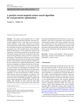
0 0.5 1 1.5 2 2.5 3
x 10
4
10
-15
10
-10
10
-5
10
0
10
5
FEs
Error
f13
PSCS
CS
PSO
0 0.5 1 1.5 2 2.5 3
x 10
4
10
-40
10
-30
10
-20
10
-10
10
0
10
10
FEs
Error
f14
PSCS
CS
PSO
0 0.5 1 1.5 2 2.5 3
x 10
4
10
-40
10
-30
10
-20
10
-10
10
0
10
10
FEs
Error
f15
PSCS
CS
PSO
0 0.5 1 1.5 2 2.5 3
x 10
4
10
-15
10
-10
10
-5
10
0
10
5
FEs
Error
f16
PSCS
CS
PSO
0 0.5 1 1.5 2 2.5 3
x 10
4
10
-35
10
-30
10
-25
10
-20
10
-15
10
-10
10
-5
10
0
10
5
FEs
Error
f17
PSCS
CS
PSO
0 0.5 1 1.5 2 2.5 3
x 10
4
10
-14
10
-12
10
-10
10
-8
10
-6
10
-4
10
-2
10
0
10
2
FEs
Error
f18
PSCS
CS
PSO
0 0.5 1 1.5 2 2.5 3
x 10
4
-80
-70
-60
-50
-40
-30
-20
-10
FEs
Error
f19
PSCS
CS
PSO
0 0.5 1 1.5 2 2.5 3
x 10
4
-80
-70
-60
-50
-40
-30
-20
-10
FEs
Error
f20
PSCS
CS
PSO
Fig. 2 The convergence rate of the function error values on f 13– f 20
rior or equal to the GL-25 on some functions. For the GL-25
algorithm, it can be better than PSCS for the GL-25 algo-
rithm for the function f 01, f 02, f 07, f 08 and f 16 on 30D.
For the 50D problem, the PSCS is similar with the DE algo-
rithm on some functions. However, the DE algorithm only
can better PSCS on the function f 16. As far as the results
of the MABC with 30D problem, PSCS is similar with six
test functions, while the MABC is better than the PSCS algo-
rithm on one test function f 02. In the next, we will analyse
different algorithms.
First, we will compare our algorithm with the MABC
(Akay and Karaboga 2012) and GOABC (El-Abd 2012).
Modified artificial bee colony algorithm, MABC for short,
is proposed to used and applied to the real-parameter opti-
mization problem. GOABC is enhanced by combining the
concept of generalized opposition-based learning. This con-
cept is introduced through the initialization step and through
the generation jumping. The performance of the proposed
generalized opposition-based ABC (GOABC) is compared
to the performance of ABC. The functions were studied at
D = 30, and D = 50. The results are listed in Tables 5, 6, 7
and 8 after D × 10, 000 NFFEs.
As can be seen in these tables, we can find that PSCS is
better than MABC on eleven out of eighteen in the case of
30D. For the rest functions, PSCS and MABC can all find the
optimal solution except f 02. For the 50D problem, our algo-
rithm can give the best solution for all benchmark functions.
Compared with the GOABC, the PSCS also can obtain bet-
ter solution than the GOABC algorithm with 30D and 50D
except f 11. For the f 10, GOABC can obtain the best solu-
tion with 50D. For the dimensional 30, it can be deduced that
PSCS is statistically significantly better as compared to all
123
14. X. Li, M. Yin
Table 3 Best, worst, median, mean, standard deviation and success rate values achieved by CS, PSO and PSCS through 30 independent runs on
fixed dimensions
No. Dim Methods Best Worst Median Mean SD Sig.
+ f 21 2 CS 0.9980 0.9985 0.9980 0.9981 1.3647e−004 −
PSO 0.9980 0.9980 0.9980 0.9980 1.9119e−016 −
PSCS 0.9980 0.9983 0.9980 0.9980 9.9501e−005
f 22 4 CS 7.1751e−004 0.0018 0.0010 0.0011 3.3925e−004 +
PSO 5.787e−004 0.0214 7.249e−004 0.0035 0.0069 +
PSCS 7.1628e−004 0.0013 8.5650e−004 9.0847e−004 1.9201e−004
f 23 2 CS −1.0316 −1.0316 −1.0316 −1.0316 8.2950e−008 −
PSO −1.0316 −1.0316 −1.0316 −1.0316 6.5454e−016 −
PSCS −1.0316 −1.0316 −1.0316 −1.0316 6.4580e−007
f 24 2 CS 0.3979 0.3979 0.3979 0.3979 1.8927e−006 −
PSO 0.3979 0.3979 0.3979 0.3979 0 −
PSCS 0.3979 0.3985 0.3979 0.3980 2.1092e−004
f 25 2 CS 3 3 3 3 1.0058e−008 +
PSO 3 3.0011 3.0002 3.0003 2.7243e−004 +
PSCS 3 3 3 3 3.7532e−013
f 26 3 CS −3.8628 −3.8628 −3.8628 −3.8628 4.8402e−006 +
PSO −3.8628 −3.8628 −3.8628 −3.8628 2.2035e−015 −
PSCS −3.8628 −3.8628 −3.8628 −3.8628 5.8053e−007
f 27 6 CS −3.3192 −3.3013 −3.3137 −3.3130 0.0049 +
PSO −3.3219 −3.2031 −3.2031 −3.2427 0.0570 +
PSCS −3.3213 −3.3134 −3.3160 −3.3167 0.0025
f 28 4 CS −9.9828 −9.1045 −9.7448 −9.7008 0.2715 −
PSO −10.1531 −2.6304 −5.1007 −6.6281 3.0650 +
PSCS −10.0104 −8.7811 −9.3368 −9.4557 0.4223
f 29 4 CS −10.3143 −8.5449 −10.0948 −9.7808 0.6724 +
PSO −10.4029 −1.8375 −10.4029 −8.0758 3.4499 +
PSCS −10.3814 −9.7080 −10.0669 −10.0592 0.2245
f 30 4 CS −10.3571 −8.9279 −9.7901 −9.7428 0.4723 +
PSO −10.5364 −2.4217 −10.5364 −8.9789 2.9320 +
PSCS −10.5331 −9.7516 −10.3150 −10.2130 0.2574
other algorithms. Obviously, it can be seen that the PSCS is
superior to all other algorithms.
Second, PSCS was compared with two other state-of-the-
art DE variants, i.e., DE and OXDE (Wang et al. 2011a,b).
Wang et al. (2011a) proposes an orthogonal crossover oper-
ator, which is based on orthogonal design, can make a sys-
tematic and rational search in a region defined by the par-
ent solutions. Experimental results show the OXDE is very
effective. Tables 5, 6, 7 and 8 summarizes the experimen-
tal results for 30D and 50D. As can be seen in Table 5, for
the 30D problem, PSCS can obtain better solutions than DE
and OXDE. For the 50D problem, the algorithm can find the
better solutions than DE algorithm except f 10 and f 16.
Third, to evaluate the effectiveness and efficiency of
PSCS, we compare its performance with CLPSO (Liang
et al. 2006), CMA-ES (Hansen and Ostermeier 2001),
GL-25 (Garcia-Martinez et al. 2008). Liang et al. proposes
a new particle swarm optimization-CLPSO; a particle uses
the personal historical best information of all the particles to
update its velocity. Hansen and Ostermeier propose a very
efficient and famous evolution strategy. Garcia-Martinez et
al. proposes a hybrid real-coded genetic algorithm which
combines the global and local search. Each method was run
30 times on each test function. Table 5, 6, 7 and 8 summa-
rizes the experimental results for 30D and 50D. As can be
seen in these tables, PSCS significantly outperforms CLPSO,
CMA-ES, and GL-25. PSCS performs better than CLPSO,
CMA-ES, and GL-25 on 15, 15, and 13 out of 18 test function
for 30D, respectively. CLPSO and CMA-ES are superior to,
equal to PSCS on three test functions. GL-25 is superior to,
equal to PSCS on five test functions. For the 30D, the results
are shown in Table in terms of the mean, standard deviation
123
15. A particle swarm inspired cuckoo search algorithm
Table 4 Comparisons the NFFES of CS, PSO and PSOCS on 30 dimension problem
N Max_NFEES CS PSO PSCS
Mean SD SR Mean SD SR Mean SD SR
f 01 3e5 128,190 4.0888e+003 30 185,085 2.8981e+003 30 47,580 6.3385e+002 30
f 02 3e5 228,490 5.0498e+003 30 186,520 2.7211e+003 30 60,550 1.0936e+003 30
f 03 3e5 NA NA NA NA NA NA 185,020 8.7575e+003 30
f 04 3e5 NA NA NA NA NA NA 170,780 3.2987e+003 30
f 05 3e5 NA NA NA NA NA NA 295,040 1.5684e+004 3
f 06 3e5 87,880 5.7420e+003 30 165,045 7.3227e+003 30 25,600 1.1728e+003 30
f 07 3e5 NA NA NA NA NA NA NA NA NA
f 08 3e5 12,660 1.4104e+003 30 69,180 8.4894e+003 30 6,300 8.2865e+002 30
f 09 3e5 NA NA NA NA NA NA 161,900 5.3299e+003 30
f 10 3e5 NA NA NA NA NA NA 185,450 4.0749e+003 30
f 11 3e5 184,350 1.8280e+004 30 261,985 5.0812e+004 12 58,620 2.0043e+003 30
f 12 3e5 NA NA NA NA NA NA 143,420 4.4293e+003 30
f 13 3e5 270,620 1.9708e+004 27 202,200 4.9934e+003 30 79,600 6.3133e+003 30
f 14 3e5 245,070 3.8154e+004 30 213,685 4.6077e+004 24 40,790 1.0795e+003 30
f 15 3e5 158,460 5.1055e+003 30 219,180 4.3058e+004 24 45,590 7.5048e+002 30
f 16 3e5 NA NA NA 192,275 5.5779e+003 30 299,290 1.7816e+003 6
f 17 3e5 144,990 3.9761e+003 30 190,010 3.9215e+004 28 41,600 1.1756e+003 30
f 18 3e5 NA NA NA 250,250 4.2935e+004 18 97,770 1.0551e+003 30
f 19 3e5 NA NA NA NA NA NA 141,030 5.8638e+003 30
f 20 3e5 NA NA NA NA NA NA NA NA NA
f 21 1e4 5,800 3.0422e+003 24 5,450 3.0733e+003 27 5,100 2.1155e+003 30
f 22 1e4 NA NA NA NA NA NA NA NA NA
f 23 1e4 3,420 8.0249e+002 30 8,465 2.1612e+003 17 3,820 1.2752e+003 30
f 24 1e4 3,970 9.7758e+002 30 9,455 1.0468e+003 11 7,530 1.9630e+003 24
f 25 1e4 3,330 1.2884e+003 30 9,585 1.4704e+003 5 2,780 5.6529e+002 30
f 26 1e4 3,060 8.4747e+002 30 1,525 5.3812e+002 30 2,350 9.1560e+002 30
f 27 1e4 9,990 31.622 3 NA NA NA 9,030 1.5004e+003 12
f 28 1e4 NA NA NA NA NA NA NA NA NA
f 29 1e4 NA NA NA NA NA NA NA NA NA
f 30 1e4 NA NA NA NA NA NA NA NA NA
of the solutions obtained in the 30 independent runs by each
algorithm. From the Table 6, we can find that the PSCS pro-
vides better solutions than other algorithms on 17, 14, and
14 out of 18 test functions for 50D, respectively.
Finally, to show the effective of our algorithm further,
we increase the function evaluation number up to at least
2,000,000 with the dimension 50. Since the problem solv-
ing success of some algorithms used in the tests strongly
depends on “the size of the population”, the size of the popu-
lation is 30. Then, the proposed algorithm is compared with
eight well-known algorithms. Based on the above experi-
ments, the CLPSO, GL-25 and CMA-ES are discarded from
experiments. MABC and GOABC are still in the compared
algorithms. For the DE algorithm, we use the CoDE (Wang
et al. 2011a,b) instead of the standard DE and OXDE because
it is very effective compared with other well-known algo-
rithms. Simultaneously, we also add some well-known algo-
rithms, such as bat algorithm (BA) (Yang and Gandomi Amir
2012), backtracking search optimization algorithm (BSA)
(Civicioglu 2012, 2013a,b), Bijective/Surjective version of
differential search algorithm (BSA, SDS) (Civicioglu 2012,
2013a,b). BSA uses three basic genetic operators: selection,
mutation and crossover to generate trial individuals. This
algorithm has been shown better than some well-known algo-
rithms. DS algorithm simulates the Brownian-like random-
walk movement used by an organism to migrate and its per-
formance is compared with the performances of the classical
methods. These two algorithms are high performance meth-
ods. Therefore, we add these two algorithms in our experi-
ments. The statistical results are calculated in Tables 9 and
10. As observed in Table 9, the proposed PSCS obtains good
results in some benchmark test functions. The analysis and
123
16. X. Li, M. Yin
Table 5 Comparisons with other algorithms on 30 dimension problem
F f 1 f 2 f 3
Algorithm Mean SD p value Mean SD p value Mean SD p value
MABC 7.2133e−044 4.7557e−044 1 3.6944e−031 1.6797e−031 −1 3.8170e+003 1.0130e+003 1
GOABC 5.4922e−016 1.4663e−016 1 6.5650e−016 3.2782e−016 1 3.3436e+003 1.6035e+003 1
DE 1.8976e−031 2.3621e−031 1 6.7922e−016 3.8931e−016 1 3.5495e−005 3.0922e−005 1
OXDE 5.7407e−005 2.3189e−005 1 0.0089 0.0015 1 2.6084e+003 456.6186 1
CLPSO 1.2815e−023 5.8027e−024 1 1.4293e−014 3.9883e−015 1 6.4358e+002 1.5270e+002 1
CMA-ES 5.9151e−029 1.0673e−029 1 0.0132 0.0594 1 1.5514−026 3.6118e−027 −1
GL-25 8.2615e−232 0 −1 3.1950e−038 1.3771e−037 −1 3.5100 6.1729 1
FA 9.0507e−004 1.9291e−004 1 0.0162 0.0034 1 0.0060 0.0021 1
FPA 2.9882e−009 4.2199e−009 1 1.5300e−005 6.7334e−006 1 5.4833e−007 1.3205e−006 1
PSCS 9.6819e−051 1.0311e−050 – 1.2865e−028 5.2708e−029 – 2.3503e−009 2.0191e−009 –
F F4 F5 F6
Algorithm Mean SD p value Mean SD p value Mean SD p value
MABC 0.0849 0.0106 1 25.1824 1.3538 1 0 0 0
GOABC 1.2109 3.8285 1 38.6234 24.6906 1 0 0 0
DE 0.0644 0.1704 1 3.0720 0.5762 1 0 0 0
OXDE 0.4925 0.2268 1 23.8439 0.4515 1 0 0 0
CLPSO 2.5647 0.2958 1 5.6052 3.6231 1 0 0 0
CMA-ES 3.9087e−015 4.7777e−016 −1 1.8979 2.4604 1 0 0 0
GL-25 0.3726 0.2910 1 22.0314 1.4487 1 0 0 0
FA 0.0393 0.0134 1 30.9577 16.9374 1 0 0 0
FPA 1.7694 0.6656 1 20.8044 13.2997 1 0 0 0
PSCS 4.1096e−009 1.8666e−009 – 1.6879 2.4024 – 0 0 –
F F7 F8 F9
Algorithm Mean SD p value Mean SD p value Mean SD p value
MABC 0.0114 0.0022 1 4.6951e−093 1.0199e−092 1 60.4535 4.4675 1
GOABC 0.0108 0.0046 1 8.5567e−017 7.5688e−017 1 0 0 0
DE 0.0048 0.0012 1 3.5903e−060 1.1354e−059 1 139.0106 33.9803 1
OXDE 0.0065 0.0014 1 9.4201e−025 1.7803e−024 1 93.9627 8.9225 1
CLPSO 0.0053 0.0010 1 9.2601e−080 1.0938e−079 1 3.1327e−012 5.6853e−012 1
CMA-ES 0.2466 0.0813 1 6.7414e−020 6.7206e−020 1 2.2754e+002 64.3046 1
GL-25 0.0014 5.8267e−004 −1 1.0375e−322 0 −1 19.5817 6.2866 1
FA 0.0203 0.0131 1 1.3939e−008 7.4786e−009 1 34.4259 12.6178 1
FPA 0.0119 0.0065 1 5.0197e−029 1.0228e−028 1 27.7686 5.2689 1
PSCS 0.0037 0.0015 – 4.3501e−156 9.0819e−156 – 0 0 –
F f 10 f 11 f 12
Algorithm Mean SD p value Mean SD p value Mean SD p value
MABC 44.3808 4.8644 1 0 0 0 2.0518e+003 644.3215 1
GOABC 0 0 0 0.0115 0.0178 1 11.8438 37.4534 1
DE 98.3747 27.4538 1 0 0 0 5.1481e−009 1.6278e−008 1
OXDE 70.3559 10.5847 1 0.0029 0.0035 1 1.9799e+003 697.7371 1
CLPSO 1.2276e−010 7.2195e−011 1 4.9404e−015 6.2557e−015 1 0 0 0
123
17. A particle swarm inspired cuckoo search algorithm
Table 5 continued
F f 10 f 11 f 12
Algorithm Mean SD p value Mean SD p value Mean SD p value
CMA-ES 2.4720e+002 45.9514 1 0.0014 0.0036 1 5.5215e+003 8.1119e+002 1
GL-25 34.8904 6.9122 1 2.9753e-015 7.6569e-015 1 3.5905e+003 9.6997e+002 1
FA 43.7334 19.5903 1 0.0021 5.5807e-004 1 5.2300e+003 389.8672 1
FPA 33.0036 6.2419 1 0.0116 0.0114 1 3.2972e+003 2.9941e+002 1
PSCS 0 0 – 0 0 – 0 0 –
F f 13 f 14 f 15
Algorithm Mean SD p value Mean SD p value Mean SD p value
MABC 7.9936e−015 0 1 1.5705e−032 2.8850e−048 0 1.3498e−032 2.8850e−048 0
GOABC 3.0020e−014 1.0296e−014 1 0.0124 0.0393 1 2.9888e−006 9.4515e−006 1
DE 5.1514e−015 1.4980e−015 1 2.1772e−032 7.0712e−033 1 3.8520e−032 3.9614e−032 1
OXDE 0.0026 4.6523e−004 1 2.5482e−006 1.1609e−006 1 1.9809e−005 8.4309e−006 1
CLPSO 1.1306e−012 2.7237e−013 1 1.1760e−024 8.6371e−025 1 7.3255e−024 4.5667e−024 1
CMA-ES 19.5117 0.1664 1 0.0103 0.0319 1 5.4936e−004 0.0024 1
GL-25 8.9173e−014 1.4217e−013 1 2.1809e−031 7.7133e−031 1 2.1243e−031 3.8884e−031 1
FA 0.0073 9.9154e−004 1 0.0114 0.0122 1 6.7341e−004 2.9108e−004 1
FPA 1.5676 1.0199 1 0.0622 0.1347 1 7.3713e−004 0.0028 1
PSCS 4.4409e−015 0 – 1.5705e−032 2.8849e−048 – 1.3498e−032 2.8849e−048 –
F f 16 f 17 f 18
Algorithm Mean SD p value Mean SD p value Mean SD p value
MABC 0.0053 0.0012 1 1.3498e-031 0 0 0 0 0
GOABC 3.5689e−012 8.2904e−012 −1 3.5846e−016 6.6160e−017 1 3.5527e−015 5.0243e−015 1
DE 0.0027 0.0045 1 1.3498e−031 0 0 0 0 0
OXDE 0.0253 0.0018 1 2.6546e−006 7.4999e−007 1 33.7129 2.0843 1
CLPSO 1.1762e−004 3.8038e−005 1 6.5838e−025 3.447e−025 1 0 0 0
CMA-ES 0.1496 0.2721 1 0.3164 1.3381 1 2.7869 1.9945 1
GL-25 9.9252e−006 3.8464e−005 −1 2.2374e−028 9.6446e−028 1 0.0044 0.0020 1
FA 0.0701 0.0557 1 0.2336 0.3232 1 22.1799 1.6093
FPA 0.0775 0.1881 1 0.0073 0.0283 1 2.8863 0.8868 1
PSCS 1.0285e−004 2.4428e−005 – 1.3498e−031 0 – 0 0 –
discussion of the experimental results are given in the fol-
lowing section:
1. For MABC and GOABC, the proposed PSCS clearly per-
forms better than competitors on seven test functions (f 3,
f 4, f 5, f 9, f 10, f 13, f 16). MABC offers the best perfor-
mance on two test functions (f 2 and f 12) and GOABC
can obtain better solution on F7. For the rest functions,
our algorithm can provide the similar solutions with these
algorithms. From the Table 10, we can draw a conclu-
sion that the outstanding of the proposed algorithm is
attributed to its new updated search method. Therefore,
PSCS has the good exploitation ability in terms of solving
these functions.
2. For the algorithm CoDE, the experimental results show
that the proposed algorithm is better than CoDE on eight
test functions including f 2, f 5, f 9, f 10, f 14, f 15, f 16
and f 17. For the function f 3, f 4, and f 12, the CoDE
outperforms our algorithm on these functions. For the
rest functions f 1, f 6, f 7, f 8, f 11 and f 18, both algo-
rithms can obtain the same results. The reason is that
the best solution in the current population is used in our
algorithm, which indicates that the proposed algorithm
has the pleasurable exploration ability.
123
18. X. Li, M. Yin
Table 6 Rank of different algorithms on 30D problem
F MABC GOABC DE OXDE CLPSO CMA-ES GL-25 FA FPA PSCS
f 01 3 7 4 9 6 5 1 10 8 2
f 02 2 4 5 8 6 9 1 10 7 3
f 03 10 9 4 8 7 1 6 5 3 2
f 04 5 8 4 7 10 1 6 3 9 2
f 05 8 9 3 7 4 2 6 10 5 1
f 06 1 1 1 1 1 1 1 1 1 1
f 07 7 6 3 5 4 10 1 9 8 2
f 8 3 9 5 7 4 8 1 10 6 2
f 9 7 1 9 8 3 10 4 6 5 1
f 10 7 1 9 8 3 10 5 6 4 1
f 11 1 9 1 8 5 6 4 7 10 1
f 12 6 4 3 5 1 10 8 9 7 1
f 13 3 4 2 7 6 10 5 8 9 1
F14 1 9 3 6 5 7 4 8 10 1
F15 1 6 3 7 5 8 4 9 10 1
F16 6 1 5 7 4 10 2 8 9 3
F17 1 6 3 7 5 10 4 9 8 1
F18 1 5 1 10 1 7 6 9 8 1
Average 4.0556 5.5000 3.7778 6.9444 4.4444 6.9444 3.8333 7.6111 7.0556 1.5000
3. For the algorithm FA, BA, BSA, BDS and SDS, our algo-
rithm can obtain the best solutions on all test functions
compared with the FA and BA. For the BSA, it only
can provide the better solution than our algorithm on test
function f 12. BDS and SDS are two different versions
of differential search algorithm. From the results, these
algorithms can provide very similar results with our algo-
rithm. For BDS, it can provide the better solutions on
function f 12 and f 17. For the f 1, f 6, f 8, f 10, f 11,
f 14, f 15, f 17 and f 18, our algorithm can give the best
solutions. For the SDS, our algorithm can perform better
than this algorithm on the test functions including f 2,
f 3, f 4, f 5, f 7, f 9, f 11, f 13, f 16 and f 17. For the
f 12, SDS can give the better solution. This is attributed
to that our algorithm uses different search methods to
enlarge the search space.
Summarizing the above statements, PSCS can prevent the
nest falling into the local solution, reduce evolution proposed
significantly and convergence faster.
5 Application to real world problems
In this section, we will use the algorithm to solve two famous
real-world optimizations to verify the efficacy of the pro-
posed algorithm.
5.1 Chaotic system
The following part of this section describes the chaotic sys-
tem. Let
˙X = F(X, X0, θ0) (16)
be a continuous nonlinear chaotic system, where X =
(x1, x2, . . . , xN ) ∈ Rn the state vector of the chaotic system
is, ˙X is the derivative of X and X0 denotes the initial state.
The θ0 = (θ10, θ20, . . . , θd0) is the original parameters.
Suppose the structure of system (16) is known, then the
estimated system can be written as
˙X = F(X, X0, ˜θ) (17)
where ˜X = (˜x1, ˜x2, . . . , ˜xN ) ∈ Rn denotes the state vector,
and ˜θ = ( ˜θ1, ˜θ2, . . . , ˜θd) is a set of estimated parameters.
Based on the measurable state vector X = (x1, x2, . . . ,
xN ) ∈ Rn, we define the following objective function or
fitness function
f ( ˜θn
i ) =
W
t=0
(x1(t) − xn
i,1(t))2
+ · · · + (xN (t) − xn
i,N (t))2
(18)
where t = 0, 1, . . . , W. The goal of estimating the parame-
ters of chaotic system (17) is to find out the suitable value of
˜θn
i so that fitness function (18) is globally minimized.
To evaluate the performance of our algorithm, we applied
it to the chaotic system as the standard benchmark. Lorenz
123
19. A particle swarm inspired cuckoo search algorithm
Table 7 Comparisons with other algorithms on 50 dimension problem
F f 1 f 2 f 3
Algorithm Mean SD p value Mean SD p value Mean SD p value
MABC 3.0941e−032 1.3476e−032 1 1.1029e−025 5.4166e−026 1 4.0654e+004 3.8946e+003 1
GOABC 9.6227e−016 4.1880e−016 1 1.8941e−015 5.7908e−016 1 1.8008e+004 1.1428e+004 1
DE 6.4438e−035 9.0934e−035 1 7.6202e−018 4.5051e−018 1 2.1434 1.3166 1
OXDE 4.0583e−006 1.7326e−006 1 0.0016 3.8530e−004 1 1.2537e+004 1.7127e+003 1
CLPSO 6.0841e−011 2.3352e−011 1 1.6721e−007 2.7779e−008 1 9.7209e+003 1.3183e+003 1
CMA-ES 1.1135e−028 1.8896e−029 1 0.0011 0.0052 1 7.2663e−026 1.1403e−026 −1
GL-25 3.6608e−164 0 −1 2.9368e−008 1.2813e−007 1 1.8173e+002 1.8525e+002 1
FA 0.0035 7.2415e−004 1 0.0756 0.0335 1 0.2429 0.0671 1
FPA 2.6443e−005 2.3912e−005 1 5.0326e−005 1.9679e−005 1 0.3083 0.1823 1
PSCS 1.5045e−063 9.7749e−064 – 3.0332e−035 1.3784e−035 – 4.0249e−005 1.8619e−005 –
F F4 F5 F6
Algorithm Mean SD p value Mean SD p value Mean SD p value
MABC 6.3271 0.6280 1 48.4641 10.0716 1 0 0 0
GOABC 2.0933 5.7658 1 46.6914 0.1364 1 0 0 0
DE 4.7399 1.8562 1 21.2158 2.2015 1 0 0 0
OXDE 3.7553 1.3748 1 42.5529 2.6007 1 0 0 0
CLPSO 10.4321 0.5326 1 72.4622 26.3377 1 0 0 0
CMA-ES 5.7282e−015 6.1633e−016 −1 0.1993 0.8914 −1 0 0 0
GL-25 9.5680 1.9727 1 41.0062 0.8413 1 0 0 0
FA 0.0855 0.0071 1 95.9064 72.5433 1 0 0 0
FPA 8.6147 9.0588 1 50.4389 25.1110 1 0.2 0.4472 1
PSCS 1.5855e−010 1.1521e−010 – 11.5491 1.3832 – 0 0 –
F F7 F8 F9
Algorithm Mean SD p value Mean SD p value Mean SD p value
MABC 0.0258 0.0034 1 2.7185e−053 3.0991e−053 1 200.3499 12.3649 1
GOABC 0.01458 0.0047 1 1.0793e−016 9.4372e−017 1 0 0 0
DE 0.0062 0.0011 1 1.0607e−024 3.3519e−024 1 224.8962 54.7317 1
OXDE 0.0103 0.0034 1 4.5549e−024 1.3807e−023 1 146.7573 9.1273 1
CLPSO 0.0158 0.0042 1 1.2511e−057 2.0673e−057 1 3.4997 1.1701 1
CMA-ES 0.2713 0.1054 1 1.8078e−017 1.5782e−017 1 3.8022e+002 79.2564 1
GL-25 0.0050 0.0012 1 1.0745e−274 0 −1 49.0380 9.0639 1
FA 0.0121 0.0054 1 2.2465e−008 9.2175e−009 1 81.9855 26.1505 1
FPA 0.0578 0.0221 1 1.4688e−024 2.7240e−024 1 45.2255 11.8221 1
PSCS 0.0042 8.6491e−004 – 1.3546e−236 0 – 0 0 –
F f 10 f 11 f 12
Algorithm Mean SD p value Mean SD p value Mean SD p value
MABC 163.7688 12.2769 1 0 0 0 7.7211e+003 655.7639 1
GOABC 0 0 −1 0.00591 0.0080 1 11.8913 37.4370 1
DE 194.0885 35.8132 1 0 0 0 189.5013 186.8508 1
OXDE 137.0397 9.4330 1 5.0143e−006 2.3346e−006 1 69.8963 105.5689 1
CLPSO 9.0885 2.3566 1 3.9804e−008 4.7773e−008 1 3.3105e−011 9.1473e−012 1
123
20. X. Li, M. Yin
Table 7 continued
F f 10 f 11 f 12
Algorithm Mean SD p value Mean SD p value Mean SD p value
CMA-ES 3.8490e+002 64.6715 1 8.6266e−004 0.0026 1 9.2754e+003 1.0321e+003 1
GL-25 78.3676 22.9800 1 2.3617e−013 8.7969e−013 1 7.5250e+003 1.1652e+003 1
FA 90.0001 10.9316 1 0.0043 3.6548e−004 1 9.2466e+003 1.0012e+003 1
FPA 49.7813 14.9183 1 0.0049 0.0075 1 6.2738e+003 3.2282e+002 1
PSCS 0.0185 0.0299 – 0 0 – 1.8190e−011 1.8190e−011 –
F f 13 f 14 f 15
Algorithm Mean SD p value Mean SD p value Mean SD p value
MABC 1.9718e−014 2.3979e−015 1 2.3891e−027 3.4561e−027 1 3.0936e−028 2.5372e−028 1
GOABC 5.5244e−014 1.0860e−014 1 9.5123e−016 6.6300e−017 1 0.1303 0.2774 1
DE 6.2172e−015 1.8724e−015 1 9.4233e−033 1.4425e−048 0 1.3498e−032 2.8850e−048 0
OXDE 4.4683e−004 6.1365e−005 1 6.6657e−008 1.8656e−008 1 1.7408e−006 9.1030e−007 1
CLPSO 1.8146e−006 1.7580e−007 1 4.1795e−012 1.3277e−012 1 7.3135e−011 2.0487e−011 1
CMA-ES 19.4765 0.1470 1 0.0062 0.0191 1 0.0016 0.0040 1
GL-25 3.9945e−009 1.7822e−008 1 0.0279 0.0621 1 0.0679 0.1293 1
FA 0.0117 0.0012 1 0.3730 0.3851 1 0.0041 9.0510e−004 1
FPA 1.3134 1.2827 1 0.0769 0.1398 1 10.5293 9.8654 1
PSCS 9.4233e−033 1.4425e−048 – 9.4233e−033 1.4425e−048 – 1.3498e−032 2.8849e−048 –
F f 16 f 17 f 18
Algorithm Mean SD p value Mean SD p value Mean SD p value
MABC 0.0316 0.0024 1 1.3498e−031 0 0 0 0 0
GOABC 3.4754e−010 8.8363e−010 −1 7.5876e−016 1.0618e−016 1 2.9842e−014 1.5639e−014 1
DE 1.7682e−010 5.4624e−010 −1 1.3498e−031 0 0 0 0 0
OXDE 0.0203 0.0092 1 1.7238e−007 1.1368e−007 1 62.9351 1.9283 1
CLPSO 0.0047 0.0011 1 3.0900e−012 9.7408e−013 1 1.3296e−004 1.8833e−005 1
CMA-ES 0.7919 1.0294 1 0.4714 0.9191 1 5.5316 2.7861 1
GL-25 4.7890e−004 0.0011 −1 4.0716e−026 1.3718e−025 1 0.1393 0.0596 1
FA 1.4922 1.0389 1 0.7896 1.0041 1 39.7721 2.1286 1
FPA 6.5539e−005 7.9779e−005 −1 0.0220 0.0491 1 7.7835 1.6791 1
PSCS 0.0021 4.7521e−004 – 1.3498e−031 0 – 0 0 –
system described below was chosen to test the performance
of the algorithm. Each algorithm ran 30 times on the chaotic
system. The successive W state (W = 30) of both the esti-
mated system and the original system are used to calculate
the fitness.
The well-known Lorenz (1963) system is employed as an
example in this paper. The general expression of the chaotic
system can be described as follows:
⎧
⎨
⎩
˙x1 = θ1(x2 − x1)
˙x2 = (θ2 − x3)x1 − x2
˙x3 = x1x2 − θ3x3
(19)
where x1, x2 and x3 are the state variable, θ1, θ2 and θ3 are
unknown positive constant parameters. The original parame-
ters is θ1 = 10 θ2 = 28 and θ3 = 8/3. To simulate, we let
the parameters of the Lorenz system be θ1 = 10, θ2 = 28,
θ3 = 8/3.
To simulate this system, the successive state W is 30 and
each algorithm ran 30 times with each single runs 100 iter-
ations. Table 11 lists the statistical results of the best fitness
value, the mean value, the standard deviation and identified
parameters of Lorenz system. From Table 11, it can be seen
that the best fitness value obtained by PSCS can perform bet-
123
21. A particle swarm inspired cuckoo search algorithm
Table 8 Rank of different algorithms on 50D problem
F MABC GOABC DE OXDE CLPSO CMA-ES GL-25 FA FPA PSCS
f 01 4 6 3 8 7 5 1 10 9 2
f 02 2 4 3 9 6 8 5 10 7 1
f 03 10 9 5 8 7 1 6 3 4 2
f 04 7 4 6 5 10 1 9 3 8 2
f 05 7 6 3 5 9 1 4 10 8 2
f 06 1 1 1 1 1 1 1 1 10 1
f 07 8 6 3 4 7 10 2 5 9 1
f 8 4 9 5 7 3 8 1 10 6 2
f 9 8 1 9 7 3 10 5 6 4 1
f 10 8 1 9 7 3 10 5 6 4 2
f 11 1 10 1 6 5 7 4 8 9 1
f 12 8 3 5 4 2 10 7 9 6 1
f 13 3 4 2 7 6 10 5 8 9 1
F14 3 4 1 6 5 7 8 10 9 1
F15 3 9 1 5 4 6 8 7 10 1
F16 8 2 1 7 6 9 4 10 3 5
F17 1 5 1 7 6 9 4 10 8 1
F18 1 4 1 10 5 7 6 9 8 1
Average 4.8333 4.8889 3.3333 6.2778 5.2778 6.6667 4.7222 7.5000 7.2778 1.5556
ter than CS, and PSO. The mean of identified parameters by
PSCS is more accurate than those identified by CS and PSO.
5.2 Application to spread spectrum radar poly-phase code
design problem
Thespreadspectrumradarpoly-phasecodedesignproblemis
a very famous problem of optimal design (Das and Suganthan
2010). The problem can be defined as follows:
Global min f (X) = max(ϕ1(X), ϕ2(X), . . . , ϕ2m(X))
where X = (x1, . . . , xD) ∈ RD|0 ≤ x j ≤ 2π, j = 1, . . . ,
D and m = 2D − 1.
ϕ2i−1(X) =
D
j=i
cos
⎛
⎝
j
k=|2i− j−1|+1
xk
⎞
⎠, i = 1, 2, . . . , D
ϕ2i (X) = 0.5 +
D
j=i+1
cos
⎛
⎝
j
k=|2i− j|+1
xk
⎞
⎠,
i = 1, 2, . . . , D − 1
ϕm+i (X) = −ϕi (X), i = 1, 2, . . . , m.
Table 12 shows the best, worst, median, mean and the stan-
dard deviation values obtained by three algorithms through
30 independent runs. As can be seen in this table, we can find
that our algorithm can achieve superior performance over the
other algorithms. It can also demonstrate that our algorithm
is a very effective algorithm for optimization problem.
6 Conclusions
In this paper, we propose a new cuckoo search algorithm-
inspired particle swarm optimization to solve the global opti-
mization problems with continuous variables. In our paper,
the proposed algorithms modify the update strategy through
add the neighborhood individual and best individual to bal-
ance the exploitation and exploration of the algorithm. In the
first part, the algorithm uses the neighborhood individual to
enhance the diversity of the algorithm. In the second part, the
algorithm uses two new search strategies changing by a ran-
dom probability rule to balance the exploitation and explo-
ration of the algorithm. In other aspect, our algorithm has a
very simple structure and thus is easy to implement. To verify
the performance of PSCS, 30 benchmark functions chosen
from literature are employed. The results show that the pro-
posed PSCS algorithm clearly outperforms the basic CS and
PSO algorithm. Compared with some evolution algorithms
(CLPSO, CMA-ES, GL-25, DE, OXDE, ABC, GOABC, FA
and FPA) from literature, we find our algorithm is superior
to or at least highly competitive with these algorithms. In
the last, experiments have been conducted on two real-world
problems. Simulation results and comparisons demonstrate
that the proposed algorithm is very effective.
123
22. X. Li, M. Yin
Table 9 Coherent comparisons with other algorithms on 50 dimension problem
F f 1 f 2 f 3
Algorithm Mean SD p value Mean SD p value Mean SD p value
MABC 0 0 0 0 0 −1 2.1639e+004 3.4719e+003 1
GOABC 4.590e−008 1.026e−007 1 1.2910e−011 2.860e−011 1 4.1824e+004 2.1844e+004 1
CoDE 0 0 0 2.6431e−176 0 1 8.9463e−048 2.2692e−047 −1
FA 7.465e−101 7.142e−102 1 0.0083 0.0163 1 2.0373e−025 3.1539e−026 1
BA 2.7120-005 3.023e−006 1 1.5945e+004 3.2499e+004 1 3.2420e+002 7.2495e+002 1
BSA 2.201e−261 0 1 3.5564e−148 8.4640e−148 1 1.6969e−005 2.2606e−005 1
BDS 0 0 0 2.6645e-177 0 1 0.0754 0.0705 1
SDS 0 0 0 3.6358e−206 0 1 2.5610e−005 1.9755e−005 1
PSCS 0 0 − 1.1924e−272 0 − 6.7446e−046 4.2013e−046 −
F F4 F5 F6
Algorithm Mean SD p value Mean SD p value Mean SD p value
MABC 8.294e−012 7.675e−012 1 36.2419 31.0792 1 0 0 0
GOABC 0.3459 0.1311 1 4.98838e+002 8.0716e+002 1 0 0 0
CoDE 9.093e−048 2.567e−047 −1 0.3987 1.2271 1 0 0 0
FA 0.0532 0.0251 1 45.8660 0.8307 1 0 0
BA 32.0319 5.5715 1 9.5638 2.4789 1 2.9988e+004 8.0771e+003 1
BSA 0.0309 0.0266 1 0.9966 1.7711 1 0 0 0
BDS 2.293e−013 3.594e−013 1 9.8809 20.8574 1 0 0 0
SDS 1.319e−016 1.755e−016 1 5.2646e−027 1.8936e−026 1 0 0 0
PSCS 5.830e−020 1.301e−019 − 2.5590e−028 2.0639e−028 − 0 0 −
F F7 F8 F9
Algorithm Mean SD p value Mean SD p value Mean SD p value
MABC 0.0113 0.0023 1 0 0 0 27.4042 56.7605 1
GOABC 2.100e−004 1.124e−004 −1 1.4851e−017 1.2626e−017 1 1.1952 2.1599 1
CoDE 0.0013 7.535e−004 0 0 0 0 0.4975 0.9411 1
FA 0.0349 0.0272 1 1.1005e−008 4.3442e−009 1 93.9239 41.6611 1
BA 0.0699 0.0159 1 1.8885e−010 2.4897e−011 1 1.0328e+002 22.6817 1
BSA 0.0044 0.0010 1 0 0 0 0.3482 0.6674 1
BDS 0.0020 6.841e−004 1 0 0 0 0.0497 0.2224 1
SDS 0.0019 3.597e−004 −1 0 0 0 0.8457 1.2616 1
PSCS 0.0013 2.771e−004 0 0 − 0 0 −
F f 10 f 11 f 12
Algorithm Mean SD p value Mean SD p value Mean SD p value
MABC 117.4553 7.6507 1 0 0 0 1.8190e−011 0 −1
GOABC 5.0011e−009 7.2382e−009 1 0.0024 0.0055 1 23.6877 52.9674 −1
CoDE 1.8000 1.3219 1 0 0 0 1.8190e−011 0 −1
FA 1.042e+002 9.859 1 2.220e−017 4.965e−017 1 8.457e+003 3.328e+002 1
BA 4.2235e+002 1.5171e+002 1 18.7555 41.9249 1 1.0584e+004 8.503e+002 1
BSA 0 0 0 0.0013 0.0033 1 5.9219 26.4836 −1
BDS 0 0 0 0 0 0 5.9219 26.4836 −1
SDS 0 0 0 8.6131e−004 0.0038 1 1.8190e−011 0 −1
123
23. A particle swarm inspired cuckoo search algorithm
Table 9 continued
F f 13 f 14 f 15
Algorithm Mean SD p value Mean SD p value Mean SD p value
PSCS 0 0 − 0 0 − 47.3753 64.8713 −
MABC 1.1191e−014 2.0167e−015 1 9.4233e−033 1.4425e−048 0 1.3498e−032 2.8850e−048 0
GOABC 5.2013e−004 9.2477e−004 1 1.6304e−004 3.6458e−004 1 0.0624 0.1396 1
CoDE 4.4409e−015 0 0 0.0031 0.0139 1 5.4937e−004 0.0025 1
FA 5.3468e−014 1.1621e−014 1 0.0128 0.0137 1 3.3674e−005 3.0565e−005 1
BA 16.7048 0.7936 1 13.8561 19.4668 1 1.3728e+002 13.3091 1
BSA 2.7355e−014 4.5343e−015 1 9.4233e−033 1.4425e−048 0 5.4936e−004 0.0024 1
BDS 1.0302e−014 3.3157e−015 1 9.4233e−033 1.4425e−048 0 1.3498e−032 2.8850e−048 0
SDS 1.3500e−014 2.9330e−015 1 9.4233e−033 1.4425e−048 0 2.3488e−032 4.2383e−032 1
PSCS 4.4409e−015 0 − 9.4233e−033 0 1.3498e−032 0 −
F f16 f17 f18
Algorithm Mean SD p value Mean SD p value Mean SD p value
MABC 5.9746e−028 1.7753e−027 1 1.3498e−031 0 0 0 0 0
GOABC 4.2093e−006 8.8854e−006 1 6.0368e−011 1.3498e−010 1 3.1674e−005 6.4256e−005 1
CoDE 1.0894e−014 4.3789e−014 1 0.0055 0.0246 1 0 0 0
FA 0.5996 0.2157 1 0.9538 1.6373 1 39.5324 1.4778 1
BA 4.8754 1.4660 1 1.7640e+002 2.0049e+002 1 62.7109 6.6955 1
BSA 2.8981e−023 8.9652e−023 1 1.8921e−031 4.5315e−032 1 2.8422e−015 5.8320e−015 1
BDS 7.9231e−033 3.5346e−032 −1 1.3498e−031 0 0 0 0 0
SDS 4.1633e−017 1.8619e−016 1 2.4043e−031 4.2263e−031 1 0 0 0
PSCS 4.4980e−030 9.1888e−030 − 1.3498e−031 0 − 0 0 −
Table 10 Rank of different algorithms on 50D problem for a coherent comparison
F MABC GOABC CoDE FA BA BSA BDS SDS PSCS
f 01 1 8 1 7 9 6 1 1 1
f 02 1 7 5 8 9 6 4 3 2
f 03 8 9 1 3 7 4 6 5 2
f 04 5 8 1 7 9 6 4 3 2
f 05 7 9 3 8 5 4 6 2 1
f 06 1 1 1 1 9 1 1 1 1
f 07 8 1 2 9 7 6 5 4 2
f 8 1 7 1 9 8 1 1 1 1
f 9 7 6 4 8 9 3 2 5 1
f 10 8 5 6 7 9 1 1 1 1
f 11 1 8 1 5 9 7 1 6 1
f 12 1 6 1 8 9 4 4 1 7
f 13 4 8 1 7 9 6 3 5 1
F14 1 6 7 8 9 1 1 1 1
F15 1 8 6 5 9 6 1 4 1
F16 3 7 6 8 9 4 1 5 2
f 17F 1 6 7 8 9 4 1 5 1
F18 1 7 1 8 9 6 1 1 1
Average 3.333 6.5000 3.0556 6.8889 8.5000 4.2222 2.4444 3.000 1.6111
123
24. X. Li, M. Yin
Table 11 The statistical results of the best fitness value, the mean value, the standard deviation and identified parameters of Lorenz system
Algorithm Means of best fitness SD of best fitness Mean value and best value obtained (in brackets) of identified parameters
θ1 θ2 θ3
PSCS 2.4995e−006 2.93660e−006 10.0000 (10.0002) 28.0000 (28.0000) 2.6667 (2.6667)
CCS 1.81E−04 1.66E−04 9.9984 (10.0000) 27.9997 (28.0000) 2.6666 (2.6665)
PSO 0.11788 0.268094 10.1667 (9.9999) 28.0105 (27.9999) 2.6684 (2.6666)
Table 12 The best, worst,
median, mean and the standard
deviation values obtained by
PSCS, CS and PSO through 30
independent runs
Dimension Algorithm Best Worst Median Mean SD
D = 19 PSCS 0.5 0.5133 0.5 0.5037 0.0059
CS 0.6868 0.8987 0.7749 0.7759 0.0872
PSO 0.5594 0.8090 0.5922 0.6477 0.1107
D = 20 PSCS 0.5 0.5982 0.5 0.5288 0.0435
CS 0.7645 0.9133 0.8750 0.8469 0.0710
PSO 0.5 1.0581 0.8274 0.7870 0.2084
In this paper, we only consider the global optimization.
The algorithm can be extended to solve other problems such
as constrained optimization problems.
Acknowledgments This research is fully supported by Opening Fund
of Top Key Discipline of Computer Software and Theory in Zhejiang
Provincial Colleges at Zhejiang Normal University under Grant No.
ZSDZZZZXK37 and the Fundamental Research Funds for the Cen-
tral Universities Nos. 11CXPY010. Guangxi Natural Science Founda-
tion (No. 2013GXNSFBA019263), Science and Technology Research
Projects of Guangxi Higher Education (No.2013YB029), Scientific
Research Foundation of Guangxi Normal University for Doctors.
References
Agrawal S, Panda R, Bhuyan S, Panigrahi BK (2013) Tsallis entropy
based optimal multilevel thresholding using cuckoo search algo-
rithm. Swarm Evol Comput 11:16–30
Akay B, Karaboga D (2012) A modified artificial bee colony algorithm
for real-parameter optimization. Inf Sci 192:120–142
Burnwal S, Deb S (2013) Scheduling optimization of flexible manu-
facturing system using cuckoo search-based approach. Int J Adv
Manuf Technol 64(5–8):951–959
Civicioglu P (2012) Transforming geocentric cartesian coordinates to
geodetic coordinates by using differential search algorithm. Com-
put Geosci 46(229–247):2012
Civicioglu P (2013a) Backtracking search optimization algorithm for
numerical optimization problems. Appl Math Comput 219(8121–
8144):2013
Civicioglu P (2013b) Circular antenna array design by using evolution-
ary search algorithms. Progr Electromagn Res B 54:265–284
Civicioglu P, Besdok E (2013) A conceptual comparison of the cuckoo-
search, particle swarm optimization, differential evolution and arti-
ficial bee colony algorithms. Artif Intell Rev 39(4):315–346
Das S, Suganthan PN (2010) Problem definitions and evaluation criteria
for CEC 2011 competition on testing evolutionary algorithms on
real world optimization problems. Jadavpur University, India and
Nanyang Technological University, Singapore, Technical Report-
Technical Report
Dey N, Samanta S, Yang XS et al (2013) Optimisation of scaling factors
in electrocardiogram signal watermarking using cuckoo search. Int
J Bio Inspir Comput 5(5):315–326
Durgun ˙I, Yildiz AR (2012) Structural design optimization of vehicle
componentsusingcuckoosearchalgorithm.MaterTest 54(3):185–
188
Ehsan V, Saeed T (2013) Improved cuckoo search for reliability opti-
mization problems. Comput Ind Eng 64(1):459–468
El-Abd M (2012) Generalized opposition-based artificial bee colony
algorithm. IEEE Congr Evol Comput (CEC) 2012:1–4
Gandomi A, Yang X, Alavi A (2013) Cuckoo search algorithm: a meta-
heuristic approach to solve structural optimization problems. Eng
Comput 29:17–35
Garcia-Martinez C, Lozano M, Herrera F, Molina D, Sanchez AM
(2008) Global and local real-coded genetic algorithms based
on parent-centric crossover operators. Eur J Oper Res 185:
1088–1113
Goghrehabadi A, Ghalambaz M, Vosough A (2011) A hybrid power
series—cuckoo search optimization algorithm to electrostatic
deflection of micro fixed-fixed actuators. Int J Multidiscip Sci Eng
2(4):22–26
Hansen N, Ostermeier A (2001) Completely derandomized self adap-
tation in evolution strategies. Evol Comput 9(2):159–195
Kennedy J, Eberhart R (1995) Particle swarm optimization. Proc IEEE
Int Conf Neural Netw 4(2):1942–1948
Layeb A (2011) A novel quantum inspired cuckoo search for knapsack
problems. Int J Bio Inspir Comput 3:297–305
Li XT, Wang JN, Yin MH (2014) Enhancing the performance of cuckoo
search algorithm using orthogonal learning method. Neural Com-
put Appl 24(6):1233–1247
Liang JJ, Qin AK, Suganthan PN, Baskar S (2006) Comprehen-
sive learning particle swarm optimizer for global optimization
of multimodal functions. IEEE Trans Evol Comput 10(3):281–
295
Lorenz EN (1963) Deterministic nonperiodic flow. J Atmos Sci 20:130–
141
Ouaarab A, Ahiod B, Yang XS (2014) Discrete cuckoo search algorithm
for the travelling salesman problem. Neural Comput Appl 24(7–
8):1659–1669
Storn R, Price K (1997) Differential evolution—a simple and efficient
heuristic for global optimization over continuous space. J Glob
Optim 11:341–359
123
25. A particle swarm inspired cuckoo search algorithm
Tuba M, Subotic M, Stanarevic N (2011) Modified cuckoo search algo-
rithm for unconstrained optimization problems. In: Proceeding of
the 5th European conference on European computing conference
(ECC’11), pp 263–268
Walton S, Hassan O, Morgan K, Brown MR (2011) Modified cuckoo
search: a new gradient free optimisation algorithm Chaos. Solitons
Fractals 44:710–718
Wang Y, Cai ZX, Zhang QF (2011a) Enhancing the search ability
of differential evolution through orthogonal crossover. Inf Sci
18(1):153–177
Wang Y, Cai Z, Zhang Q (2011b) Differential evolution with compos-
ite trial vector generation strategies and control parameters. IEEE
Trans Evol Comput 15(1):55–66
Yang XS (2009) Firefly algorithms for multimodal optimization. In:
Stochastic algorithms: foundations and applications, SAGA 2009.
Lecture Notes in Computer Sciences, vol 5792, pp 169–178
Yang XS (2012) Flower pollination algorithm for global optimiza-
tion. In: Unconventional computation and natural computation.
Springer, Berlin, pp 240–249
Yang XS, Deb S (2009) Cuckoo search via Levy flights. World Congress
on nature & biologically inspired computing (NaBIC 2009). IEEE
Publication, USA, pp 210–214
Yang XS, Gandomi Amir H (2012) Bat algorithm: a novel approach for
global engineering optimization. Eng Comput 29(5):464–483
Yildiz AR, Saitou KN (2011) Topology synthesis of multicompo-
nent structural assemblies in continuum domains. J Mech Des
133(1):011008
Yildiz AR, Solanki KN (2012) Multi-objective optimization of vehicle
crashworthiness using a new particle swarm based approach. Int J
Adv Manuf Technol 59(1–4):367–376
Yildiz AR (2012) A comparative study of population-based optimiza-
tion algorithms for turning operations. Inf Sci 210:81–88
Yildiz AR (2013) A new hybrid artificial bee colony algorithm for robust
optimal design and manufacturing. Appl Soft Comput 13(5):2906–
2912
Yildiz AR (2013) Cuckoo search algorithm for the selection of opti-
mal machining parameters in milling operations. Int J Adv Manuf
Technol 64(1–4):55–61
123