


![JPEG Encoding
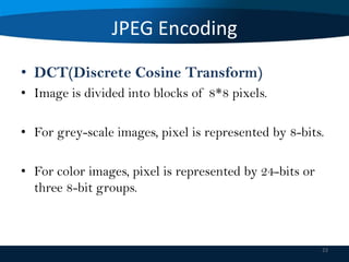
• DCT takes an 8*8 matrix and produces another 8*8
matrix and its values represent by this equation:
T[i][j] = 0.25 C(i) C(j) ∑ ∑ P[x][y] Cos(2x+1)iπ/16
* Cos (2y+1)jπ/16
i = 0, 1, …7, j = 0, 1, …7
C(i) = 1/√2, i =0
= 1 otherwise
T contains values called ‘Spatial frequencies’
24](https://image.slidesharecdn.com/datacompresionme-131111065752-phpapp02/85/Data-compression-24-320.jpg)
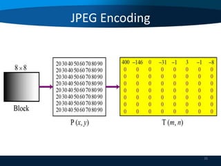
![JPEG Encoding
• T[0][0] is called the DC coefficient, related to
average values in the array, Cos 0 = 1
• Other values of T are called AC coefficients, cosine
functions of higher frequencies
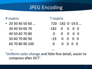
Case 1: all P’s are same, image of single color with no variation
at all, AC coefficients are all zeros.
Case 2: little variation in P’s, many, not all, AC coefficients are
zeros.
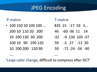
Case 3: large variation in P’s, a few AC coefficients are zeros.
25](https://image.slidesharecdn.com/datacompresionme-131111065752-phpapp02/85/Data-compression-25-320.jpg)


![JPEG Encoding
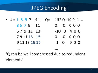
• Dividing T-elements by the same number is not
practical, may result in too much loss.
• Retain the effects of lower frequencies as much as
possible.
• To define a quantization array Q, then
Q[i][j] = Round (T[i][j] ÷ U[i][j]),
i = 0, 1,.........7, j = 0, 1, …7
31](https://image.slidesharecdn.com/datacompresionme-131111065752-phpapp02/85/Data-compression-31-320.jpg)
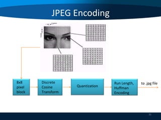

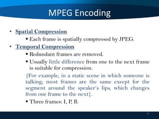


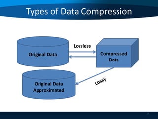
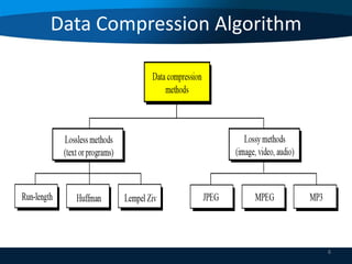
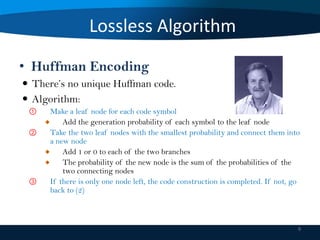
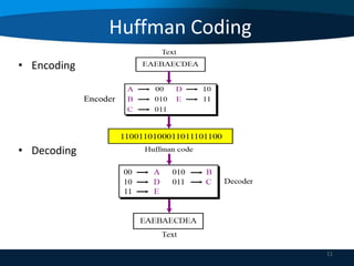
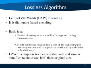
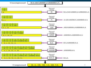
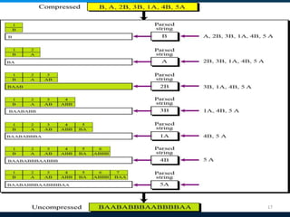
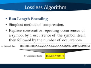
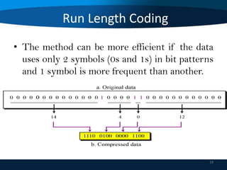
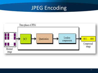
This document provides an overview of data compression techniques. It discusses lossless compression algorithms like Huffman encoding and LZW encoding which allow for exact reconstruction of the original data. It also discusses lossy compression techniques like JPEG and MPEG which allow for approximate reconstruction for images and video in order to achieve higher compression rates. JPEG divides images into 8x8 blocks and applies discrete cosine transform, quantization, and run length encoding. MPEG spatially compresses each video frame using JPEG and temporally compresses frames by removing redundant frames.