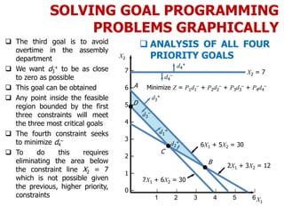
Downloaded 843 times


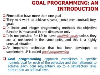
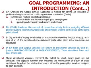
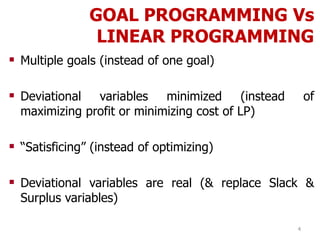
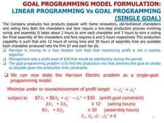

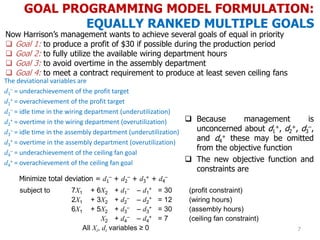
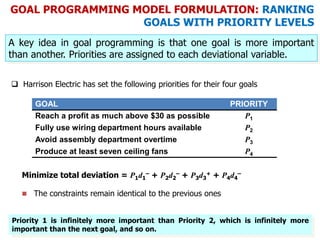
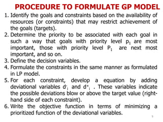
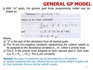
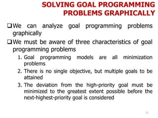
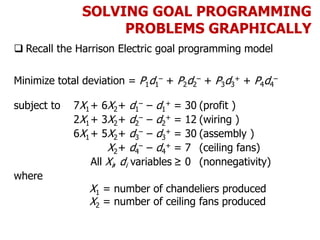
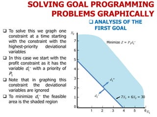
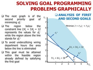


This document provides an introduction and overview of goal programming (GP). It explains that GP is useful when an organization has multiple, sometimes conflicting goals that cannot all be optimized at the same time like in linear programming. GP establishes numeric goals for each objective and attempts to achieve each goal to a satisfactory level by minimizing deviations. The document outlines the basic components of a GP model, including defining goals and constraints, assigning priority levels to goals, and introducing deviational variables. It also provides an example to illustrate how to formulate a GP model and solve it graphically or using the modified simplex method.